Appendix B
Mathematical and Statistical Foundations
This appendix supplies the formal background the main text refers to but does not derive. It is written to be read one section at a time, the section a chapter points to, rather than straight through, and every abstraction is landed in a small numerical example, two-by-two or three-by-three, computed against values a reader can check by hand or with the companion code. There are no proofs beyond sketches and no measure theory. The aim is not to teach the mathematics from nothing but to make precise the objects the methods chapters manipulate: the covariance matrices whose positive-definiteness the model demands, the likelihoods the estimators maximize, the multivariate normal that underlies the Kalman filter and the imputation model, and the Bayesian machinery Chapter 17 puts to work.
B.1 Matrix Algebra Minimum
Used in Chapters 13, 19, 25, 26, 27, and 30. A vector is an ordered list of numbers and a matrix a rectangular array; the transpose \(\mathbf{A}^\top\) exchanges rows and columns, and the product \(\mathbf{AB}\) is defined when the inner dimensions match. Three scalar summaries of a square matrix recur in the book. The determinant measures the volume the matrix scales, and it appears in every multivariate normal density; for \(\mathbf{A} = \bigl(\begin{smallmatrix} 2 & 1 \\ 1 & 3 \end{smallmatrix}\bigr)\) it is \(2\cdot 3 - 1\cdot 1 = 5\). The inverse \(\mathbf{A}^{-1}\) solves linear systems and appears in every generalized-least-squares and normal-equation expression; here it is \(\bigl(\begin{smallmatrix} 0.6 & -0.2 \\ -0.2 & 0.4 \end{smallmatrix}\bigr)\), and one may check that \(\mathbf{A}\mathbf{A}^{-1}\) is the identity. The eigenvalues solve \(\mathbf{A}\mathbf{v} = \lambda\mathbf{v}\) and describe the matrix’s action along its principal directions; for \(\mathbf{A}\) they are \(3.618\) and \(1.382\). That both eigenvalues are positive is exactly the condition that \(\mathbf{A}\) is positive definite, the property every covariance matrix must have, because a covariance matrix with a zero or negative eigenvalue implies a linear combination of variables with zero or negative variance, which is impossible; the Heywood cases of Chapters 13 and 19 and the non-positive-definite warnings of the SEM chapters are exactly failures of this condition. Eigenvalues carry more of the book’s weight than any other matrix idea: the stationarity of a vector-autoregression in Chapter 25 is the requirement that the eigenvalues of its transition matrix lie inside the unit circle, the drift matrix of the continuous-time model in Chapter 27 is stable when its eigenvalues have negative real parts, and the functional principal components of Chapter 30 are the eigenvectors of a covariance operator. The matrix exponential \(e^{\mathbf{A}t}\), which propagates the continuous-time model of Chapter 27, is computed numerically rather than by hand and is available in the Matrix package. Block matrices, in which a large matrix is partitioned into submatrices, organize the joint covariance of observed and latent parts in the state-space and imputation models, and the conditioning formula of Section B.4 is stated in their terms.
B.2 Expectation Algebra
Used in Chapters 13, 19, and throughout. The expectation \(E[X]\) is the mean, the variance \(\mathrm{Var}[X] = E[(X-E[X])^2]\) the spread, and the covariance \(\mathrm{Cov}[X,Y]\) their joint variation. The workhorse rule, from which the implied-covariance derivations of the growth-model chapters are built, is the variance of a linear combination: for constants \(a\) and \(b\), \(\mathrm{Var}[aX + bY] = a^2\mathrm{Var}[X] + b^2\mathrm{Var}[Y] + 2ab\,\mathrm{Cov}[X,Y]\). With \(\mathrm{Var}[X]=4\), \(\mathrm{Var}[Y]=1\), and \(\mathrm{Cov}[X,Y]=1.2\), the variance of the difference \(X-Y\) is \(4 + 1 - 2(1.2) = 2.6\), the calculation behind every change-score variance in the book. The law of total variance, \(\mathrm{Var}[Y] = E[\mathrm{Var}[Y\mid G]] + \mathrm{Var}[E[Y\mid G]]\), decomposes an outcome’s variance into a within-group and a between-group part, and it is precisely the decomposition that defines the intraclass correlation of the multilevel chapters: the between-group variance over the total is the share of variance that lies between clusters, the dyadic intraclass correlation of Chapter 35 and the school-level variance of Chapter 34 being instances.
B.3 Likelihood
Used in Chapters 13, 16, and throughout estimation. The likelihood is the probability of the observed data read as a function of the parameters, and its logarithm, the log-likelihood, is what estimators maximize because sums are easier than products and the maximizer is the same. The maximum-likelihood estimator has, under regularity conditions this appendix states but does not prove, two properties the book relies on: it is consistent, converging to the truth as the sample grows, and it is asymptotically normal, so that its sampling distribution is approximately normal with a variance given by the inverse of the Fisher information, which is the curvature of the log-likelihood at its peak. Figure B.1 shows a log-likelihood surface for a normal sample: the estimate sits at the peak, and the curvature there, sharp along a well-identified direction and flat along a poorly-identified one, is the information that becomes the standard error. Three model-comparison quantities follow from the likelihood. The likelihood-ratio test compares nested models by twice the difference in their maximized log-likelihoods, referred to a chi-square distribution whose degrees of freedom are the difference in parameter counts, valid when the models are nested and the larger is correctly specified. The Akaike and Bayesian information criteria penalize the maximized log-likelihood by a function of the parameter count, the Akaike criterion by twice it and the Bayesian criterion by the parameter count times the log sample size, so that the Bayesian criterion penalizes complexity more heavily in large samples; both are used for non-nested comparison, with the caveats the mixture chapter presses. The restricted maximum likelihood of Chapter 13 maximizes a modified likelihood that accounts for the estimation of the fixed effects, which is why its variance estimates are less biased and why likelihood-ratio tests of fixed effects must not use it. A persistent source of confusion, the different deviance conventions across packages, is resolved in Table B.1.
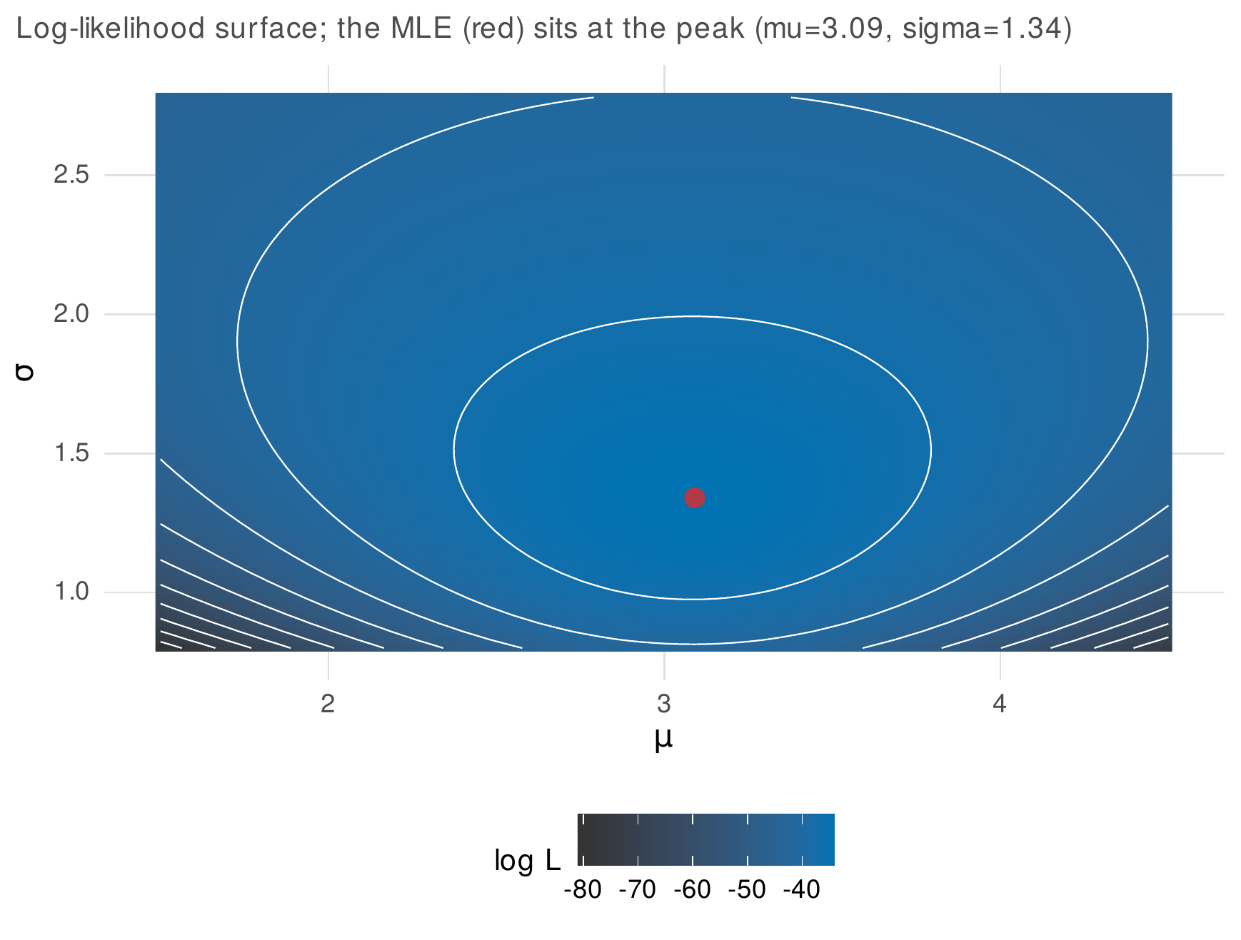
Note. The log-likelihood of a normal sample as a function of its mean and standard deviation, with the maximum-likelihood estimate at the peak. The curvature at the peak, steep in a well-identified direction and shallow in a poorly-identified one, is the Fisher information, and its inverse is the estimator’s sampling variance. Standard errors are read from this curvature, which is why a flat likelihood, a poorly-identified model, yields large standard errors.
Table B.1. Deviance and Information-Criterion Conventions
| Quantity | Definition | Caution |
|---|---|---|
| Deviance | \(-2 \times\) log-likelihood | Some packages report \(-2\ell\), some \(\ell\); check the sign and factor |
| LRT statistic | \(2(\ell_1 - \ell_0)\) | Nested models; use ML not REML for fixed-effect tests |
| AIC | \(-2\ell + 2k\) | \(k\) counts all estimated parameters, including variances |
| BIC | \(-2\ell + k\log n\) | The effective \(n\) is ambiguous in multilevel models |
Note. The single most common error in reading model output across packages is a sign or factor-of-two mismatch in the reported deviance, followed by using a REML fit for a likelihood-ratio test of a fixed effect, which is invalid because REML likelihoods of models with different fixed parts are not comparable.
B.4 The Multivariate Normal
Used in Chapters 6, 16, 17, and 26. The multivariate normal distribution, with mean vector \(\boldsymbol{\mu}\) and covariance matrix \(\boldsymbol{\Sigma}\), is the joint distribution most of the book’s models assume for their random parts, and its density, whose exponent is the quadratic form \(-\tfrac{1}{2}(\mathbf{x}-\boldsymbol{\mu})^\top\boldsymbol{\Sigma}^{-1}(\mathbf{x}-\boldsymbol{\mu})\), is where the inverse and determinant of Section B.1 earn their place. Its defining convenience is that its conditional distributions are also normal, with a mean that adjusts linearly toward the conditioning value and a variance that shrinks. For a bivariate normal with unit variances and correlation \(0.6\), conditioning the second variable on the first taking the value \(1.5\) gives a conditional mean of \(0.6 \times 1.5 = 0.90\) and a conditional variance of \(1 - 0.6^2 = 0.64\), down from the marginal \(1\), and Figure B.2 shows the geometry: the elliptical contours of the joint density, and the narrower slice that conditioning produces. This conditioning is the engine of two book methods. The Kalman filter of Chapter 26 is a repeated application of the normal conditioning formula, updating a belief about a latent state as each observation arrives; the multiple-imputation model of Chapter 6 draws the missing entries from their conditional normal given the observed, which is the same formula read as a prediction with noise. The Mahalanobis distance, the quadratic form itself, measures how far a point sits from the mean in units that account for the covariance, and it underlies multivariate outlier detection.
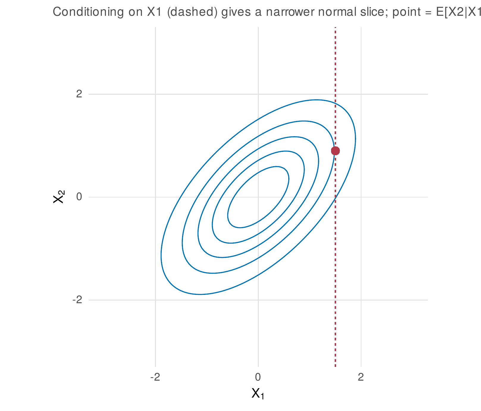
Note. The elliptical contours of a bivariate normal density with correlation \(0.6\). Conditioning on the first variable (the dashed vertical line) restricts attention to a slice, whose distribution is again normal with a mean shifted toward the conditioning value and a variance smaller than the marginal. This normal-in, normal-out property is what makes the Kalman filter and the normal imputation model tractable.
B.5 Bayesian Essentials
Used in Chapter 17 (the practice; this section is the math). Bayesian inference treats the parameters as random and updates a prior distribution into a posterior by Bayes’ theorem, the posterior being proportional to the likelihood times the prior. When the prior and likelihood are chosen to match, the update is closed-form, and the normal-normal case is the one to hold in mind: with a normal prior on a mean, of prior mean \(0\) and prior variance \(1\), and normal data of sample mean \(2\) from ten observations with known variance \(4\), the posterior mean is a precision-weighted average of the prior mean and the data mean, here \(1.429\), and the posterior variance is \(0.286\), smaller than either source alone because the data and prior each add information. The posterior mean lies between the prior mean of \(0\) and the data mean of \(2\), pulled toward the data as the sample grows and toward the prior as the prior tightens, which is the shrinkage the multilevel and small-sample chapters exploit. Most real models are not conjugate, and the posterior is then explored by Markov chain Monte Carlo, a method that draws a dependent sequence of parameter values whose long-run distribution is the posterior; convergence, the assurance that the chain has reached and is exploring that distribution, is assessed by the diagnostics of Chapter 17, the potential scale reduction factor and the effective sample size. This section is deliberately thinner than Chapter 17, which puts the machinery to work; it supplies the definitions the chapter assumes.
B.6 Notation Registry
Table B.2 is the book’s symbol registry, the meaning of each recurring symbol with the chapters that use it. Notation is kept consistent across the whole book: persons are indexed by \(i\) and occasions by \(t\), the outcome for person \(i\) at occasion \(t\) is \(y_{it}\), and the between-person and within-person components introduced in Chapter 1 keep their meaning everywhere. Where a chapter introduces a local symbol, the deviation is noted in that chapter and here.
Table B.2. The Symbol Registry
| Symbol | Meaning | Chapters |
|---|---|---|
| \(i, t\) | Person index; occasion index | all |
| \(y_{it}\) | Outcome for person \(i\) at occasion \(t\) | all |
| \(\beta\) | Fixed-effect (population) coefficient | 13–15 |
| \(b_i, u_i\) | Random effect for person \(i\) | 13–16 |
| \(\boldsymbol{\Sigma}, \mathbf{G}, \mathbf{R}\) | Covariance; random-effect; residual covariance | 13, 19 |
| \(\phi\) | Autoregressive coefficient | 24–27 |
| \(\lambda\) | Factor loading; eigenvalue; smoothing penalty | 18, 25, 30 |
| \(\rho\) | Correlation | throughout |
| \(\theta\) | Generic parameter vector; latent ability | 16, 34 |
| \(\ell(\theta)\) | Log-likelihood | 13, 16 |
| \(\pi_k\) | Mixing proportion of class \(k\) | 22 |
| \(h(t), S(t)\) | Hazard; survivor function | 29 |
Note. The registry is the book’s shared vocabulary. Consistency of notation across chapters is a deliberate aid to the reader who moves between methods: a random effect is \(b_i\) whether it sits in a growth model or a diary model, and an autoregressive coefficient is \(\phi\) whether the series is a single subject’s or a person’s within a multilevel model.