Chapter 1
Studying Change: Why Within-Person Processes Require Their Own Methods
Change is the reason this book exists. Before we estimate a single parameter, we need to be clear about what change is, whose change we are talking about, and why the ordinary tools of cross-sectional research, however well they serve their purpose, answer a different question than the one a longitudinal researcher is usually asking.
Learning Objectives
After working through this chapter, you should be able to: (1) classify a research question as concerning level, systematic change, variability, dynamics, or the timing of events; (2) explain why an association that holds across people need not hold within a person, and construct a concrete counterexample; (3) define ergodicity in informal terms and state the two conditions under which a group-level structure equals an individual-level structure; (4) distinguish the timescale of a psychological process from the timescale of a study design, and explain why the mismatch matters; (5) locate the part of this book appropriate to a given description of data and question; and (6) articulate why adding measurement occasions changes what can be estimated, so that two occasions license a statement about the amount of change, three or more license a statement about its shape, and many occasions license a statement about its dynamics.
1.1 One Question, Four Studies
Consider a question that almost every reader will find familiar: does stress affect sleep? The question sounds simple, and in one sense it is. Yet the moment we try to gather data to answer it, we discover that “does stress affect sleep” is not one question but a family of related questions, and that the design we choose silently decides which member of the family we are permitted to answer. Figure 1.1 shows the same substantive question realized in four common designs, and it is worth studying before reading on, because the entire logic of this book is contained in the contrast among its four panels.
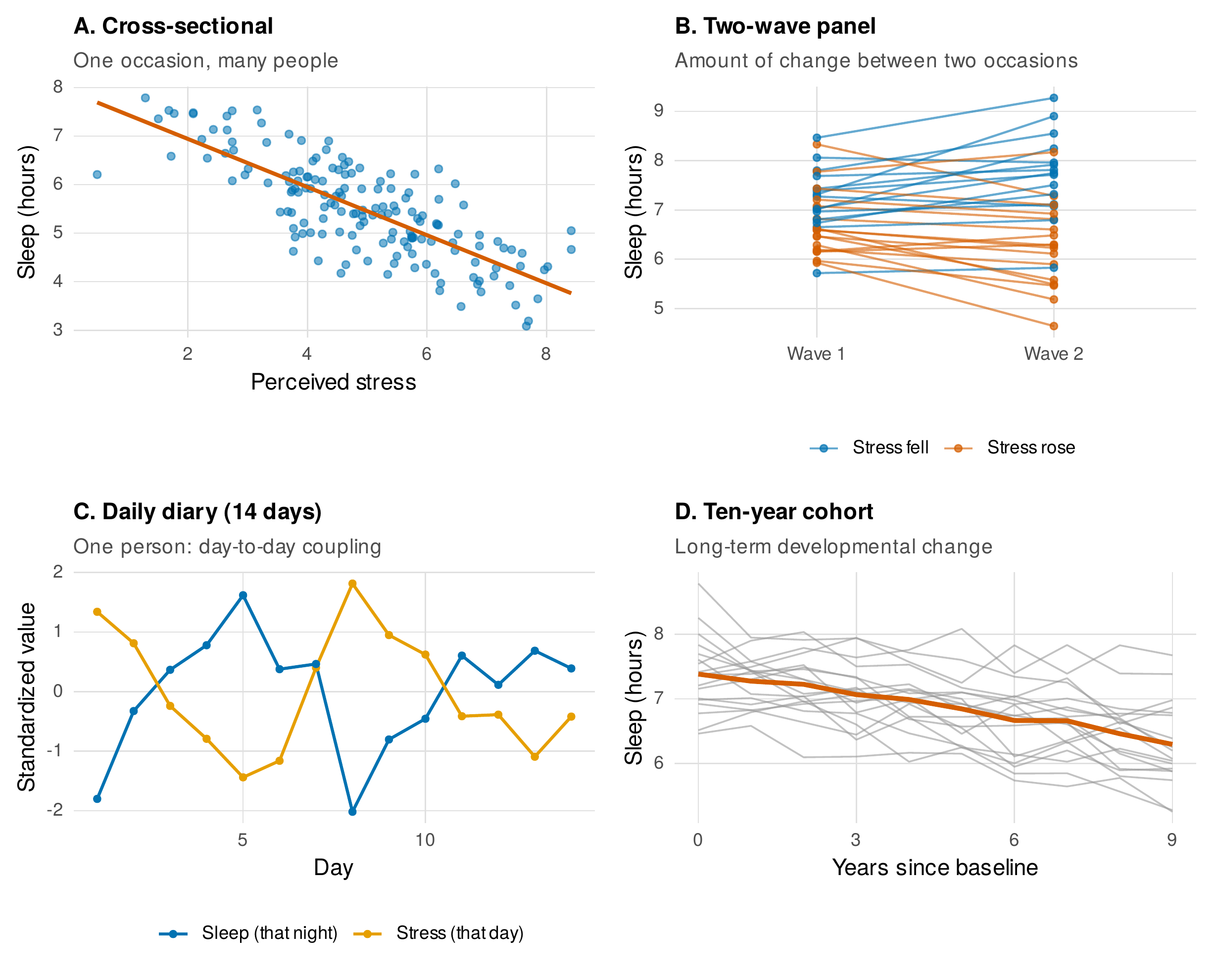
Note. Each panel displays simulated data. Panel A shows one observation per person measured on a single occasion. Panel B shows the same people measured on two occasions, with lines connecting each person’s two values. Panel C shows one person measured on fourteen consecutive days. Panel D shows a sample of people followed across ten years. The four panels are not competing analyses of one dataset; they are four different data structures, each estimating a different quantity.
In Panel A, a cross-sectional study, each person contributes a single pair of values: how stressed they are and how much they sleep, measured once. The negative slope tells us that people who report more stress tend, on average, to sleep less. This is a statement about differences between people. It says nothing about what would happen to any particular person’s sleep if their stress were to rise, because no person in the study was ever observed to change. In Panel B, a two-wave panel study, the same people are measured twice, and now each person contributes a small piece of within-person information: the direction in which their sleep moved as their stress moved. In Panel C, a fourteen-day daily diary, a single person is measured repeatedly, and the question becomes explicitly intraindividual: on the days this person is more stressed than usual, do they sleep less than usual? In Panel D, a ten-year cohort study, the question is developmental: as people age across a decade, how does their sleep change, and do people differ in that change?
The four panels share an x axis and a y axis, but they do not share an estimand, that is, the quantity the study is actually estimating. Panel A estimates a between-person association. Panel C estimates a within-person association. Panels B and D estimate change, but change of different kinds and over different timescales. It is entirely possible for these quantities to disagree, and in psychology they frequently do. A central discipline this book asks of you is to state, for any analysis, whose variance an effect lives in: the variance between people, the variance within a person over time, or some blend of the two. That single habit of mind, asking whose variance, will reorganize how you read the empirical literature.
1.2 A Taxonomy of Change Questions
Questions about change come in identifiable families, and it is more useful to learn the families than to memorize a catalogue of methods, because the family determines the method and not the other way around. Five families recur throughout psychology and the social sciences, and every chapter of this book can be located within them.
The first family concerns level and group differences over time. Here the researcher asks whether the average value of an outcome differs across groups or across occasions: whether a treatment group reports lower depression than a control group at each week of a trial, or whether average life satisfaction shifts after a major life transition such as retirement. The second family concerns the form and rate of systematic change, usually called growth. The researcher asks not merely whether an outcome changed but what the trajectory of change looks like: whether vocabulary rises linearly or with diminishing returns across the elementary school years, and whether children who begin lower grow faster or slower than their peers. The third family treats within-person variability as a quantity of substantive interest in its own right. Rather than asking about a person’s average level, the researcher asks how much a person fluctuates: whether mood becomes more erratic from one day to the next following a stressful event, and whether such affective instability is itself a marker of risk. The fourth family concerns within-person dynamics: the carryover, coupling, and feedback that link a person’s states across time. Does today’s rumination forecast tomorrow’s sadness? Do stress and negative affect amplify one another from moment to moment? The fifth family concerns the timing of events: how long until a patient relapses, or what predicts when a student withdraws from school. Table 1.1 lists the five families with psychological examples and points to the parts of the book that address each.
Table 1.1. Five families of change questions, with examples and locations in this book.
| Question family | Example research questions | Where in this book |
|---|---|---|
| Level and group differences over time | Do treatment and control groups differ in depression at each week? Does average well-being rise after retirement? | Part III (Ch. 10–12); Part IV (Ch. 13, 15) |
| Form and rate of systematic change (growth) | What is the shape of achievement growth across grades 3–8? Do children who start lower grow faster? | Part IV (Ch. 14); Part V (Ch. 19–20) |
| Within-person variability | Is a person’s mood more variable after a stressful life event? Is affective lability a risk marker? | Ch. 7, 16 |
| Within-person dynamics (carryover, coupling, feedback) | Does today’s rumination predict tomorrow’s sadness? Do stress and negative affect reinforce each other moment to moment? | Part VI (Ch. 23–28) |
| Timing of events (onset, relapse, dropout) | How long until a patient relapses? What predicts when students drop out? | Ch. 29 |
Note. Chapter numbers refer to the primary treatment of each question family; many families reappear in the applications chapters (Ch. 33–35).
The order of that sentence matters: questions precede models. A frequent and costly error, visible in published work and in student theses alike, is to begin from a favored technique and then bend the question to fit it. The remedy is to name the question family first and let it route you to a method, which is exactly the service Table 1.1, and the fuller decision aid at the end of this chapter, is designed to provide.
1.3 Between-Person and Within-Person Variation
The conceptual heart of this book is a decomposition so simple that it is easy to underestimate. Any repeated-measures observation can be split into a part that describes the person and a part that describes the occasion. Write \(y_{it}\) for the outcome of person \(i\) on occasion \(t\). Let \(\bar{y}_{i\cdot}\) denote that person’s own average across their occasions. Then every observation can be written as its person mean plus a within-person deviation:
The first term varies across people but is constant within a person; it carries information about between-person differences, about who is generally higher or lower. The second term varies within a person across occasions but averages to zero for each person; it carries information about within-person change and fluctuation, about when a person is higher or lower than their own norm. Correspondingly, the total variance of \(y\) partitions into a between-person component and a within-person component. Equation (1.1) is the only formula you need to carry out of this chapter, and it is the seed from which multilevel models (Chapters 13 and 23), latent growth models (Chapter 19), and the within-versus-between debates of the cross-lagged literature (Chapter 21) all grow.
The reason this decomposition deserves such emphasis is that the two components are logically independent: an association between two variables at the between-person level can differ in magnitude, and even in sign, from the association at the within-person level. This is not a statistical curiosity but a substantive commonplace. Consider caffeine and tiredness, illustrated in Figure 1.2. Across people, those who habitually consume more caffeine tend to report being more tired, because people reach for coffee precisely when they are chronically fatigued; the between-person association is positive. Yet within a person, the moments shortly after consuming caffeine are the moments of least tiredness; the within-person association is negative. The colored clouds in Figure 1.2, each a single person, all slope downward, while the dashed line through the persons’ averages slopes upward. A researcher who measured caffeine and tiredness once per person, as in a cross-sectional survey, would recover only the upward between-person pattern and might conclude, absurdly, that caffeine makes people tired.
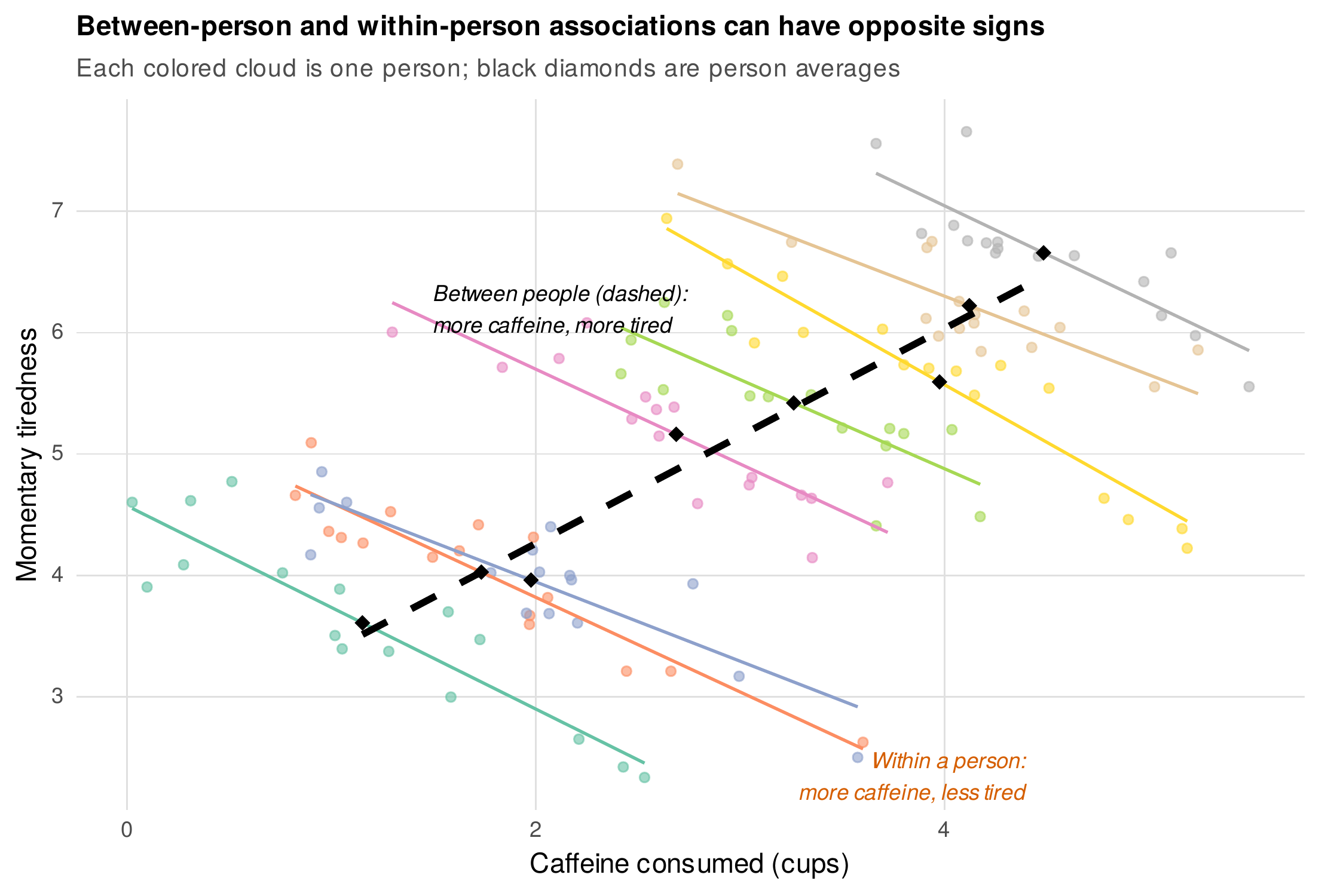
Note. Simulated illustration. Each colored point cloud represents the repeated observations of one person, and each thin colored line is that person’s within-person regression of tiredness on caffeine. Black diamonds are person averages, and the dashed black line is the between-person regression through those averages. The within-person slopes are negative; the between-person slope is positive. The underlying data are provided as reversal_demo.csv in the companion Examples folder.
This phenomenon is a version of what statisticians call Simpson’s paradox, and its longer pedigree in the social sciences runs through Robinson’s (1950) demonstration that correlations computed on group aggregates can misrepresent, or even reverse, the correlations that hold for individuals, a mistake he named the ecological fallacy. Kievit, Frankenhuis, Waldorp, and Borsboom (2013) give an accessible modern treatment aimed at psychologists, and Curran and Bauer (2011) formalize the disaggregation of between-person and within-person effects for longitudinal models, a treatment we return to in depth in Chapters 13 and 23. The practical lesson is disarmingly simple and continually forgotten: an effect estimated across people is not automatically an effect that operates within a person, and if your theory is about a process unfolding inside individuals, then between-person evidence is at best indirect and at worst misleading (Hamaker, 2012; Molenaar, 2004).
It is worth being careful about what this does and does not imply. Neither level of analysis is more real or more valid than the other; they simply answer different questions. A personnel psychologist selecting among applicants genuinely wants to know how people differ, a between-person question. A clinician deciding whether a given client’s symptoms are escalating genuinely wants to know how that client is changing relative to their own baseline, a within-person question. The error is not to study one level rather than the other; the error is to study one level and quietly report conclusions as though they applied to the other. Throughout this book we will make the disaggregation explicit, most concretely through the practice of person-mean centering introduced in Chapters 7, 13, and 23, which separates the two components of Equation (1.1) so that each can be modeled on its own terms.
Common Pitfall • cross-sectional age differences are not within-person aging
Suppose a cross-sectional study finds that older adults score lower on a processing-speed task than younger adults, and the report concludes that “cognitive speed declines with age.” The phrase quietly substitutes a within-person claim (a given person slows as they grow older) for the between-person comparison the data actually support (people who are currently older score lower than people who are currently younger). The two can diverge because the older and younger groups are different cohorts, born decades apart, differing in schooling, nutrition, and test familiarity. Only a design that observes the same people aging, as in Panel D of Figure 1.1, can license the developmental claim. Whenever you read “X changes with age” or “X increases over development,” ask whether anyone in the study was actually observed to change, or whether different people were merely compared at one time.
1.4 Ergodicity and the Idiographic–Nomothetic Axis
We can now state, more precisely, the condition under which the two levels of analysis coincide, and understand why psychology so often fails to meet it. Borrowing a term from statistical physics, a process is called ergodic when its structure computed across individuals at one moment matches its structure computed across time within one individual. When a process is ergodic, the between-person analysis and the within-person analysis converge on the same answer, and the ergonomic convenience of studying many people once, rather than one person many times, comes at no cost to inference. When a process is non-ergodic, the two analyses can diverge arbitrarily, and no amount of between-person data will reveal the within-person structure. Molenaar (2004) made this argument the centerpiece of a widely read manifesto, and the ensuing person-specific research program (Molenaar & Campbell, 2009) has reshaped how many psychologists think about generalizing from samples to individuals.
Foundations Box • when does the group equal the individual?
A repeated-measures process is ergodic (in the sense relevant here) when two conditions hold. The first is homogeneity across individuals: every person is governed by the same model with the same parameter values, so there are no meaningful individual differences in the process itself. The second is stationarity over time: each person’s process has a stable mean, variance, and pattern of associations that do not drift as time passes. If both conditions hold, the structure of variation across people at one occasion equals the structure of variation across occasions within one person, and group-level results transfer to the individual. Psychological processes routinely violate both conditions. People differ in their dynamics, breaking homogeneity, and their dynamics shift with development, learning, medication, and life events, breaking stationarity. This is not a technical nuisance to be assumed away; it is often the very phenomenon of interest. The formal statement and its consequences are developed by Molenaar (2004); an empirical demonstration that group-level estimates can badly misrepresent individuals is given by Fisher, Medaglia, and Jeronimus (2018).
The evidence that non-ergodicity is the rule rather than the exception is by now substantial. Fisher, Medaglia, and Jeronimus (2018) compared the structure of emotion and behavior estimated between persons with the structure estimated within persons across six datasets and found that the within-person variances were consistently several times larger than the between-person variances would predict, so that group-derived results systematically misstated individual-level relationships. The lesson is not the nihilistic one that group research should be abandoned. It is the disciplined one that the pooling assumptions of a model must be matched to the question. This is helpfully pictured as a continuum, shown in Figure 1.3. At one extreme sits the fully idiographic analysis of a single person, which assumes nothing about anyone else, purchased at the price of results that may not generalize. At the other extreme sits complete pooling, in which one model with one set of parameters is imposed on everyone, cheap and powerful when the homogeneity assumption holds but badly biased when it does not. Between these poles lie the workhorses of this book: random-effects models, which let each person have their own parameters while borrowing strength across persons through a shared distribution (Parts IV through VI), and person-specific models that estimate individual structures while exploiting commonalities in how those structures are shaped (Chapter 28).
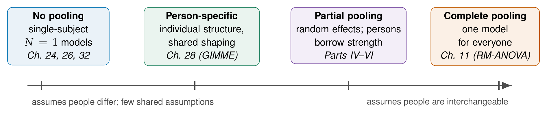
Note. Chapter numbers indicate where each stance is developed. Moving left to right, models assume progressively more homogeneity across people, gaining statistical power when the assumption holds and incurring bias when it does not. Most methods in this book occupy the partial-pooling middle, which lets individuals differ while still learning from the sample as a whole.
The older name for this tension is the contrast between the nomothetic approach, which seeks general laws that hold across individuals, and the idiographic approach, which seeks to understand the particular individual. The contrast is often presented as a philosophical either-or, but the modern resolution is more constructive: idiographic and nomothetic analyses answer different questions and can be combined, for example by estimating a model separately for each person and then asking whether the person-specific results replicate across persons (Molenaar & Campbell, 2009). Replication across individuals, rather than pooling across individuals, becomes the route to generality. We will see this idea made operational in the intensive longitudinal methods of Part VI, where the target of inference is frequently the individual and generalization is earned by showing that a dynamic holds for many individuals, one at a time.
1.5 Timescales
A process has a timescale, and a study has a timescale, and confusing the two is among the most consequential errors in longitudinal research. The timescale of a process is the rate at which it actually unfolds: cortisol responds to a stressor over minutes, mood over hours to days, marital satisfaction over months to years, and cognitive ability over decades. The timescale of a design is set by how often and for how long the researcher samples: every hour for a week, once a year for a decade, twice with six months between. When the sampling timescale is well matched to the process timescale, the data reveal the process. When it is not, the data can misrepresent the process in ways that are easy to overlook and hard to detect after the fact.
Figure 1.4 illustrates the most important of these mismatches, called aliasing. A process that genuinely cycles on roughly a weekly rhythm is sampled in two ways: densely, at daily intervals, and sparsely, at intervals of about eight days. The dense sampling recovers the weekly cycle. The sparse sampling, catching the process at a different phase each time, connects into a smooth downward line and implies a slow decline that does not exist. The sparse sampler, seeing only the red points, would report a trend; the process has no trend at all. The lesson generalizes well beyond cyclic processes. Retrospective reports, in which participants summarize how they felt “over the past month,” are a timescale decision in disguise, collapsing fast within-person variation into a single remembered average and thereby discarding exactly the dynamics that intensive designs are built to capture (Csikszentmihalyi & Larson, 1987; Stone & Shiffman, 1994). And the dependence of estimated effects on the sampling interval is not confined to descriptive displays: the size, and occasionally the sign, of a lagged effect such as “how much does stress at one moment predict negative affect at the next” depends on how much time elapses between the two moments, a problem that motivates the continuous-time models of Chapter 27.
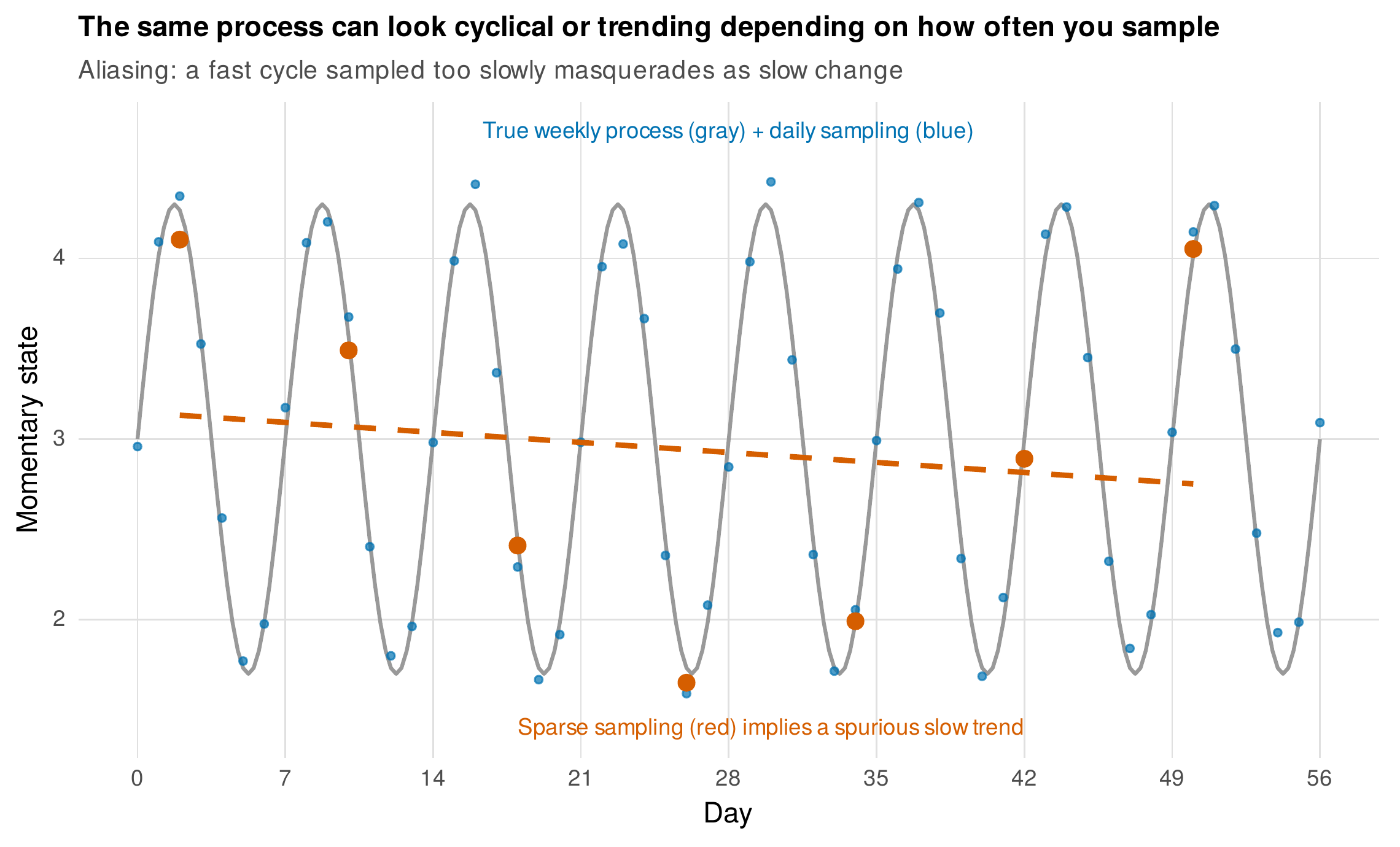
Note. Simulated illustration. The gray curve is a true process with an approximately weekly cycle. Blue points are dense (daily) samples, which recover the cycle. Red points are sparse samples taken about every eight days; the dashed red line is their linear trend, which suggests a slow decline that is an artifact of the sampling interval, not a feature of the process.
1.6 A Brief History in Five Programs
The methods in this book did not descend from a single source. They are the confluence of five research traditions that developed largely in parallel, often in different disciplines and with different vocabularies for the same ideas, which is why the modern literature is so rich in synonyms. A short historical orientation helps, not for its own sake, but because it explains why the same model appears under several names and why techniques that look unrelated are often close cousins.
The first tradition is the analysis of variance, developed for agricultural and experimental research in the early twentieth century and adapted to repeated measurements as repeated-measures and mixed-design ANOVA. It gave psychology its first systematic way to test whether means differ across occasions, and it remains the framework many researchers meet first, though its assumptions sit awkwardly with the structure of longitudinal data, a tension that motivates the multilevel alternative (Chapter 11). The second tradition is the growth-curve and structural equation modeling tradition, which reconceived change as a latent trajectory with an individually varying starting point and slope, giving rise to latent growth models and their many descendants (Chapters 19 and 20). The third tradition is the multilevel or hierarchical modeling tradition, which arose in education and sociology to handle data nested in units, students in schools, and was recognized to apply equally to occasions nested in persons, yielding the mixed-effects models at the core of Part IV. Baltes and Nesselroade (1979) articulated the rationale for longitudinal research as a distinct enterprise, and their programmatic statement still repays reading.
The fourth tradition is the time-series and idiographic tradition. Its origins in psychology trace to Cattell, Cattell, and Rhymer (1947), whose P-technique factor analysis sought the structure of a single person’s fluctuations across many occasions, an explicitly within-person factor analysis that anticipated the dynamic factor and state-space models of Chapter 26. Molenaar’s later work revived and formalized this program. Nesselroade (1991) contributed the influential image of development as a fabric with both a slowly changing “warp” and a rapidly fluctuating “woof,” motivating the measurement-burst design in which short bursts of intensive sampling are repeated at longer intervals so that fast and slow change can be studied together. The fifth tradition is the experience-sampling and ecological momentary assessment tradition, which grew from the effort to capture experience in daily life as it happens rather than in retrospect (Csikszentmihalyi & Larson, 1987; Stone & Shiffman, 1994), and which, with the arrival of smartphones and wearable sensors, has made intensive longitudinal data ordinary rather than exotic (Bolger, Davis, & Rafaeli, 2003; Hamaker & Wichers, 2017). Table 1.2 collects the most common cross-tradition synonyms, so that you can recognize the same idea when it appears in an unfamiliar dialect.
Table 1.2. A glossary of cross-tradition synonyms.
| One idea | Names it travels under |
|---|---|
| Multilevel model | hierarchical linear model (HLM), mixed-effects model, mixed model, random-coefficient model, variance-components model |
| Growth curve | latent growth model (LGM), latent trajectory model, latent curve model, random-effects growth model |
| Within-person level | level 1, occasion level, time level, state level, intraindividual |
| Between-person level | level 2, person level, trait level, interindividual |
| Autoregression | carryover, inertia, persistence, lag-1 effect |
| Experience sampling | ecological momentary assessment (EMA), ambulatory assessment, diary method, experience-sampling method (ESM) |
| Person-specific analysis | idiographic, single-subject, \(N=1\), i-level |
Note. The proliferation of names reflects the parallel development of the traditions described in the text, not deep differences among the underlying models.
1.7 How to Use This Book
Because the field is organized by tradition but your work is organized by data and question, this book provides two ways in. The first is Table 1.3, an entry matrix that crosses the structure of your data with the family of your question and points to chapters. Find the row that matches how your data are shaped, read across to the column that matches what you want to know, and begin there. The second is Figure 1.5, a fuller method-selection aid that consolidates the routing into a single diagram; it is the master map of the book, and Chapter 36 returns to it to audit, at the end of your journey, the promises this chapter has made.
Table 1.3. Entry matrix: data structure by question family, with chapter routing.
| Your data | Level / means | Growth / shape | Variability | Dynamics | Events |
|---|---|---|---|---|---|
| Two occasions | Ch. 10 | Ch. 10 | – | Ch. 21\(^{a}\) | Ch. 29 |
| 3–8 wave panel | Ch. 11, 12 | Ch. 14, 19, 20 | Ch. 7 | Ch. 21 | Ch. 29 |
| Daily diary | Ch. 23 | Ch. 14, 23 | Ch. 7, 16 | Ch. 23, 25 | Ch. 29 |
| EMA / ESM | Ch. 23 | Ch. 23, 30 | Ch. 16 | Ch. 25–28 | Ch. 29 |
| \(N=1\) long series | Ch. 24 | Ch. 24, 30 | Ch. 7, 24 | Ch. 24–26, 32 | – |
| Event times | – | – | – | – | Ch. 29 |
Note. Cells give the chapters that primarily address each combination. A dash indicates that the combination is not generally estimable from that data structure. \(^{a}\)Two-wave data support only a limited, and much-debated, form of dynamic inference; see Chapter 21. Cross-cutting concerns (missing data, measurement, estimation) apply to every cell and are treated in Chapters 3, 6, 17, and 18.
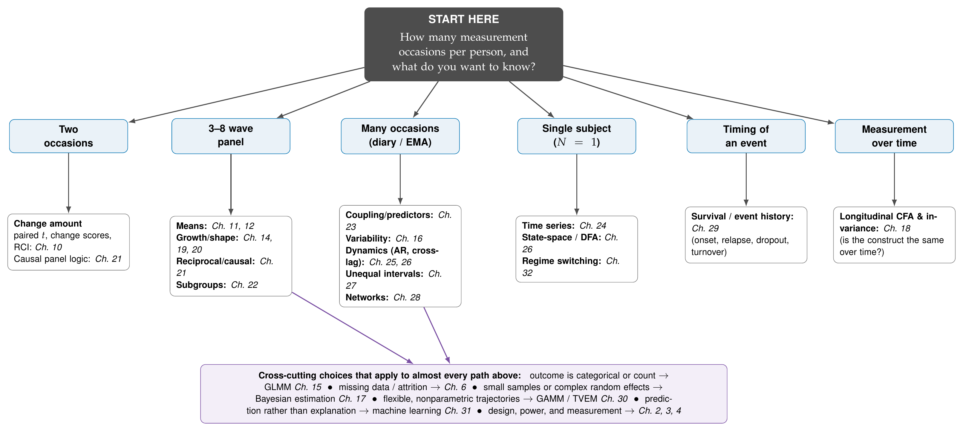
Note. Enter at the top by describing your data and question, follow the arrow to the matching category, and read the leaf for the chapters that address each question family within that data structure. The purple band lists concerns that cut across paths and are handled in dedicated chapters. This figure is the counterpart of Figure 36.1, which revisits the same map after all methods have been developed.
A few words on conventions will make the chapters that follow easier to navigate. Notation is kept consistent across the whole book: persons are indexed by \(i\) and occasions by \(t\), the outcome for person \(i\) on occasion \(t\) is \(y_{it}\), and the between-person and within-person components introduced in Equation (1.1) reappear with the same meaning everywhere. Each chapter marks its key ideas with four kinds of boxes: a Foundations box for the underlying mathematics, an In Practice box for defaults and troubleshooting, a Common Pitfall box for the errors we most want you to avoid, and a Software Note for tool-specific guidance. Every worked example draws on a small set of shared datasets so that you can follow one dataset across many methods, and all of them, together with the code that generates every figure, are provided in the companion materials described in the Software Note below. Finally, this book is modular. A one-semester course on classical longitudinal analysis might travel through Chapters 1, 5 through 8, 10 through 14, 19, 21, and 29; a course on intensive longitudinal methods might travel through Chapters 1 through 3, 5 through 7, 9, 13, 16, and 23 through 28; and a reader with data already in hand can enter directly through Table 1.3.
Software Note • the companion Examples folder and reproducibility
Every dataset in this book is simulated from a documented, seeded data-generating process, so the “truth” behind each dataset is known and you can study how well a method recovers it. This chapter uses two of them. The affect_ema dataset simulates an experience-sampling study of 120 people prompted six times a day for fourteen days, with momentary stress and affect generated by a person-specific dynamic process and realistic missingness. The school_growth dataset simulates an accelerated-cohort study of 1,200 children whose achievement is measured across four school years, stitched across three overlapping cohorts to span grades 3 through 8. Both are provided in the companion Examples folder as .rds and .csv files, together with the R scripts that generate them and codebooks documenting every variable. All analyses in this book use R; software-specific sidebars, where a package such as Mplus is the field standard, appear as needed.
1.8 Working With Change in R: A First Look
Before the formal machinery of later chapters, it is worth seeing how the ideas of this chapter appear in real data and real code. The goal here is not to fit a model, which begins in earnest in Chapter 13, but to look, because the discipline of plotting repeated-measures data before modeling it is one of the most reliable safeguards against error in longitudinal work. Every command below runs on the companion datasets and reproduces, in simplified form, the figures in this chapter.
We begin by loading the data and inspecting its shape. Repeated-measures data in this book are kept in long format, one row per person per occasion, which is the format nearly every modern longitudinal tool expects (Chapter 5 treats data management in full).
# Load the two datasets from the companion Examples folder
affect_ema    <- readRDS("Examples/data/affect_ema.rds")
school_growth <- readRDS("Examples/data/school_growth.rds")

# One row per person per occasion (long format)
head(affect_ema[, c("person", "day", "beep", "stress", "na", "pa")])
nrow(affect_ema)                 # 10,080 potential person-occasions
length(unique(affect_ema$person))# 120 people
To see what “systematic change” means, we plot the achievement trajectories of a sample of children across grades, overlaying the average trajectory. The resulting spaghetti plot, the left panel of Figure 1.6, shows individual growth as a bundle of upward lines with a clear average trend, the visual signature of a growth question.
library(ggplot2); library(dplyr)

sg_mean <- school_growth %>%
  group_by(grade) %>% summarize(achievement = mean(achievement))

ggplot(school_growth, aes(grade, achievement, group = child_id)) +
  geom_line(alpha = 0.08, color = "#0072B2") +               # individual trajectories
  geom_line(data = sg_mean, aes(group = 1),                  # average trajectory
            color = "#C15A00", linewidth = 1.3) +
  labs(x = "Grade", y = "Achievement score")
To see what “fluctuation” means, we plot a single person’s momentary negative affect across the fourteen days, as in the right panel of Figure 1.6. There is no systematic trend here; there is structured movement around the person’s own average, the visual signature of a dynamics question.
one_person <- affect_ema %>% filter(person == 4)

ggplot(one_person, aes(seq_along(na), na)) +
  geom_line(color = "#1B7F5C", na.rm = TRUE) +
  geom_point(color = "#1B7F5C", na.rm = TRUE) +
  geom_hline(yintercept = mean(one_person$na, na.rm = TRUE),
             linetype = "dashed") +                          # the person's own mean
  labs(x = "Measurement occasion", y = "Negative affect")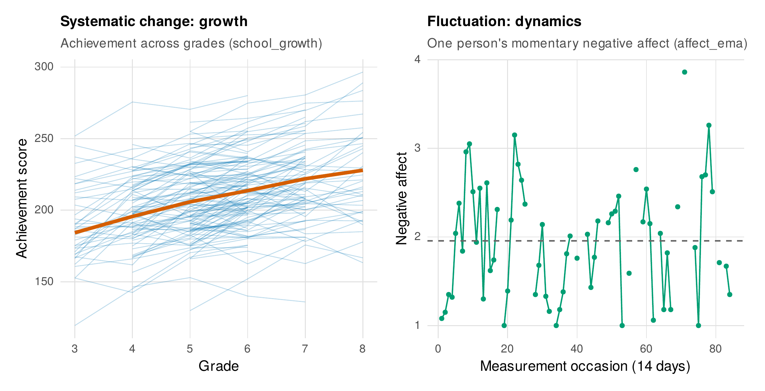
Note. Left: achievement trajectories for a sample of children from school_growth, with the average trajectory in orange; the story is one of systematic growth. Right: one person’s momentary negative affect from affect_ema across fourteen days, with the person’s own average as a dashed line; the story is one of fluctuation around a stable level. Gaps in the right panel are unanswered prompts (missing data).
Finally, we can make the between-versus-within distinction of Section 1.3 numerical rather than merely visual. Using Equation (1.1), we split each person’s momentary stress and negative affect into a person mean and a within-person deviation, then compute the association at each level. This is a descriptive decomposition, not an estimated model; the formal multilevel version, with proper standard errors, arrives in Chapter 13.
d <- affect_ema %>%
  filter(!is.na(stress), !is.na(na)) %>%
  group_by(person) %>%
  mutate(stress_pm = mean(stress),  na_pm = mean(na),         # between part
         stress_wd = stress - stress_pm,                      # within part
         na_wd     = na - na_pm) %>%
  ungroup()

# Naive pooled correlation, ignoring the person structure
cor(d$stress, d$na)                                           # ~ 0.42

# Between-person correlation (across person means)
pm <- d %>% group_by(person) %>%
  summarize(stress_pm = first(stress_pm), na_pm = first(na_pm))
cor(pm$stress_pm, pm$na_pm)                                   # ~ 0.55

# Within-person correlation (across deviations)
cor(d$stress_wd, d$na_wd)                                     # ~ 0.33
The three numbers differ, and their difference is the point. The naive correlation of about \(.42\), computed as though every observation were independent, is a blend of two distinct quantities: a between-person correlation of about \(.55\), telling us that people who are on average more stressed are on average more negative, and a within-person correlation of about \(.33\), telling us that on occasions when a person is more stressed than their own norm they are also more negative than their own norm. A researcher who reported only the pooled value would be describing neither level cleanly. A parallel decomposition of the variance of negative affect shows that only about 37% of its total variation lies between people, so that roughly 63% is within-person fluctuation, precisely the variation that a cross-sectional design discards and that the within-person methods of this book are built to model.
1.9 From Output to Prose: Writing About Change
Statistical output is not a result until it has been written for a reader, and longitudinal analyses are especially easy to describe imprecisely, because the language of everyday speech blurs the between-person and within-person distinction that the analysis works so hard to separate. This short section, which every methods chapter in this book echoes with model-specific guidance, offers a few principles for turning the displays and quantities above into defensible prose.
The first principle is to name the level explicitly. Rather than writing “stress and negative affect were correlated, \(r = .42\),” which leaves the reader to guess whose variation is meant, write two sentences that keep the levels apart. For the analysis above, a careful description reads: “Across persons, individuals who reported higher average stress also reported higher average negative affect, indicating a between-person association (\(r = .55\)). Within persons, momentary occasions of higher-than-usual stress coincided with higher-than-usual negative affect, indicating a within-person association (\(r = .33\)).” The reader now knows exactly which comparison each number refers to, and the pooled value, which corresponds to neither, is set aside rather than reported as though it summarized the relationship.
The second principle is to describe the variance structure, not only the point estimates, because in longitudinal data the allocation of variance is itself a finding. A sentence such as “approximately 63% of the variance in momentary negative affect was within-person, indicating substantial moment-to-moment fluctuation around stable individual differences” tells the reader that a within-person analysis is warranted and roughly how much signal it has to work with. The third principle is to match verbs to designs, reserving the language of change and process for data that actually observed change. Cross-sectional differences should be described with comparative language (“older participants scored lower”), not developmental language (“scores declined with age”), unless the same individuals were followed over time. The fourth principle is to state the estimand before the estimate, opening a results paragraph with the quantity being estimated (“we estimated the within-person association between stress and negative affect”) so that the number that follows is interpreted correctly from the start. These habits cost nothing and prevent a large fraction of the misreadings that longitudinal findings invite; Chapter 36 collects the full set of reporting standards, one per model family.
In Practice • how many waves do I need for which question?
The number of measurement occasions is not a matter of statistical taste; it determines what is estimable at all. Two occasions support a statement about the amount of change between them, a single difference per person, but cannot distinguish the shape of change from measurement error, and difference scores computed from two waves are notoriously unreliable (Chapter 10). Three to four occasions begin to support statements about the shape of systematic change, a linear trajectory and, with four or more, some curvature (Chapters 14 and 19). Many occasions, roughly speaking dozens or more per person, are what dynamics require, because estimating a person’s carryover, coupling, or variability demands enough within-person data points to characterize the process itself (Chapters 16 and 23 through 28). A useful slogan: two waves give you change, several waves give you a curve, and many waves give you a process. If your question concerns dynamics but your design has three waves, the honest response is to change the question or the design, not to over-interpret the model.
1.10 Common Misconceptions
A few beliefs are common enough, and consequential enough, to name directly. First, the belief that longitudinal data automatically license causal claims. Following people over time removes some alternative explanations but not others, and the reordering of variables in time is necessary, not sufficient, for causal inference; Chapter 21 treats the assumptions honestly. Second, the belief that within-person effects are simply between-person effects measured more precisely. As Figure 1.2 shows, the two can differ in sign, so they are distinct quantities, not better and worse measurements of one quantity. Third, the twin beliefs that findings from a single person cannot generalize and that group findings automatically apply to each person. Both are naive: a well-replicated single-subject result can generalize precisely because it has been shown to hold across many individuals, while a group-level result need not describe any particular individual when the process is non-ergodic (Fisher et al., 2018; Molenaar, 2004). Finally, a practical question students often ask: my data have only two waves, is this book for me? Yes. Two-wave designs have their own careful treatment (Chapter 10), figure in the causal-inference debates of Chapter 21, and share the concerns of design, measurement, and missing data that occupy Part I.
Chapter Summary
This chapter argued that longitudinal questions are not cross-sectional questions with an extra dimension, but a distinct family of questions about level, growth, variability, dynamics, and event timing, each requiring methods matched to it. Its central tool is the decomposition of any repeated measure into a between-person part and a within-person part (Equation 1.1), and its central warning is that associations at the two levels are logically independent and can even reverse in sign. Ergodicity names the rare condition, homogeneity across people and stationarity over time, under which the levels coincide; because psychological processes routinely violate it, the pooling assumptions of a model must be matched to the question rather than assumed. Timescale must likewise be matched to process, lest sparse sampling manufacture trends that do not exist. The chapter closed with the practical apparatus of the book: an entry matrix (Table 1.3) and a master decision map (Figure 1.5) that route you from data and question to method.
Where to Go Next
Readers who want to understand the designs that produce longitudinal data should continue to Chapter 2; those concerned with whether a construct even means the same thing at each occasion should look ahead to Chapters 3 and 18; and those ready to see the between-within decomposition become an estimated model should turn to Chapter 13, the multilevel foundation on which much of the book rests. The single thread to carry forward is the question posed in Section 1.1: for any effect you read or estimate, ask whose variance it lives in. Chapter 36 will return to the decision map of Figure 1.5 and audit, method by method, the promises made here.
Exercises
- 1.1 Classifying questions. For each of the following study titles, identify which of the five question families of Table 1.1 it belongs to, and justify your choice in one sentence: (a) “Does mindfulness training reduce average anxiety relative to a waitlist?”; (b) “Do adolescents whose self-esteem is more variable report more depressive symptoms?”; (c) “How long after discharge do patients first relapse?”; (d) “Does daily sleep quality predict next-day positive affect?”; (e) “What is the trajectory of reading fluency from first through fifth grade?”
- 1.2 Constructing a reversal. Using the
reversal_demo.csvdataset in theExamplesfolder, reproduce Figure 1.2. Then, from your own field, describe a pair of variables whose between-person and within-person associations plausibly differ in sign, and explain the mechanism at each level. - 1.3 What is estimable? For each of the four panels of Figure 1.1, state precisely which member of the “does stress affect sleep” question family the design can and cannot answer, and why.
- 1.4 Explaining ergodicity. In no more than 200 words, explain to a first-year undergraduate why a result that holds “on average across people” need not hold for any particular person. Use a concrete example and avoid technical vocabulary.
- 1.5 Routing your own data. Take a longitudinal dataset from your own research or a published study you admire. Using Table 1.3 and Figure 1.5, identify the chapter you would start from, and write a paragraph defending the routing, including what question family you are pursuing and why the data structure supports it.
- 1.6 Variance decomposition in R. Using
affect_ema, repeat the between-within decomposition of Section 1.8 for positive affect (pa) instead of negative affect. Report the pooled, between-person, and within-person correlations ofpawithstress, and the proportion of variance inpathat is within-person. Write two sentences describing the result following the principles of Section 1.9.
References
Baltes, P. B., & Nesselroade, J. R. (1979). History and rationale of longitudinal research. In J. R. Nesselroade & P. B. Baltes (Eds.), Longitudinal research in the study of behavior and development (pp. 1–39). Academic Press.
Bolger, N., Davis, A., & Rafaeli, E. (2003). Diary methods: Capturing life as it is lived. Annual Review of Psychology, 54, 579–616. https://doi.org/10.1146/annurev.psych.54.101601.145030
Bolger, N., & Laurenceau, J.-P. (2013). Intensive longitudinal methods: An introduction to diary and experience sampling research. Guilford Press.
Cattell, R. B., Cattell, A. K. S., & Rhymer, R. M. (1947). P-technique demonstrated in determining psycho-physiological source traits in a normal individual. Psychometrika, 12(4), 267–288. https://doi.org/10.1007/BF02288941
Csikszentmihalyi, M., & Larson, R. (1987). Validity and reliability of the Experience-Sampling Method. The Journal of Nervous and Mental Disease, 175(9), 526–536. https://doi.org/10.1097/00005053-198709000-00004
Curran, P. J., & Bauer, D. J. (2011). The disaggregation of within-person and between-person effects in longitudinal models of change. Annual Review of Psychology, 62, 583–619. https://doi.org/10.1146/annurev.psych.093008.100356
Fisher, A. J., Medaglia, J. D., & Jeronimus, B. F. (2018). Lack of group-to-individual generalizability is a threat to human subjects research. Proceedings of the National Academy of Sciences, 115(27), E6106–E6115. https://doi.org/10.1073/pnas.1711978115
Hamaker, E. L. (2012). Why researchers should think “within-person”: A paradigmatic rationale. In M. R. Mehl & T. S. Conner (Eds.), Handbook of research methods for studying daily life (pp. 43–61). Guilford Press.
Hamaker, E. L., Kuiper, R. M., & Grasman, R. P. P. P. (2015). A critique of the cross-lagged panel model. Psychological Methods, 20(1), 102–116. https://doi.org/10.1037/a0038889
Hamaker, E. L., & Wichers, M. (2017). No time like the present: Discovering the hidden dynamics in intensive longitudinal data. Current Directions in Psychological Science, 26(1), 10–15. https://doi.org/10.1177/0963721416666518
Hoffman, L. (2015). Longitudinal analysis: Modeling within-person fluctuation and change. Routledge.
Kievit, R. A., Frankenhuis, W. E., Waldorp, L. J., & Borsboom, D. (2013). Simpson’s paradox in psychological science: A practical guide. Frontiers in Psychology, 4, 513. https://doi.org/10.3389/fpsyg.2013.00513
Molenaar, P. C. M. (2004). A manifesto on psychology as idiographic science: Bringing the person back into scientific psychology, this time forever. Measurement: Interdisciplinary Research and Perspectives, 2(4), 201–218. https://doi.org/10.1207/s15366359mea0204_1
Molenaar, P. C. M., & Campbell, C. G. (2009). The new person-specific paradigm in psychology. Current Directions in Psychological Science, 18(2), 112–117. https://doi.org/10.1111/j.1467-8721.2009.01619.x
Nesselroade, J. R. (1991). The warp and woof of the developmental fabric. In R. M. Downs, L. S. Liben, & D. S. Palermo (Eds.), Visions of aesthetics, the environment, and development: The legacy of Joachim F. Wohlwill (pp. 213–240). Lawrence Erlbaum Associates.
Robinson, W. S. (1950). Ecological correlations and the behavior of individuals. American Sociological Review, 15(3), 351–357. https://doi.org/10.2307/2087176
Singer, J. D., & Willett, J. B. (2003). Applied longitudinal data analysis: Modeling change and event occurrence. Oxford University Press.
Stone, A. A., & Shiffman, S. (1994). Ecological momentary assessment (EMA) in behavioral medicine. Annals of Behavioral Medicine, 16(3), 199–202. https://doi.org/10.1093/abm/16.3.199
Wang, L. P., & Maxwell, S. E. (2015). On disaggregating between-person and within-person effects with longitudinal data using multilevel models. Psychological Methods, 20(1), 63–83. https://doi.org/10.1037/met0000030