Chapter 2
Longitudinal Research Designs: From Panel Surveys to EMA, Diary, and Ambulatory Assessment
Chapter 1 argued that questions about change require their own methods. This chapter is about the step that comes before any method: the design. What you can eventually estimate is fixed, irreversibly, by what you decide to collect, when, from whom, and how often. A design chosen well makes the analysis a matter of technique; a design chosen badly cannot be rescued by any technique at all.
Learning Objectives
After working through this chapter, you should be able to: (1) distinguish trend, panel, and cohort designs and locate any study in the two-dimensional design space of occasions by interval; (2) select among interval-, signal-, and event-contingent sampling schemes with an explicit justification; (3) state the age-period-cohort identification problem and explain how accelerated longitudinal designs address it and at what assumed cost; (4) enumerate the validity threats that arise specifically from measuring people repeatedly, and name a design countermeasure for each; (5) match the sampling timescale of a study to the timescale of the process under study; (6) specify a defensible experience-sampling protocol, including density, duration, prompt design, and a realistic compliance target; and (7) describe the logic of measurement-burst designs and of micro-randomized trials.
2.1 The Design Space
It is tempting to sort longitudinal studies into a short list of named types, but a more useful starting point is to see that every repeated-measures design occupies a position in a continuous space defined by two questions: how many times is each person measured, and how far apart are those measurements? Figure 2.1 lays out this space, with the number of occasions per person on the horizontal axis and the typical interval between occasions on the vertical axis, both on logarithmic scales because both span several orders of magnitude. A two-wave panel study sits in the upper left, with two occasions separated by months or years. A daily diary sits near the middle, with a few dozen occasions one day apart. Ecological momentary assessment sits lower and to the right, with hundreds of occasions separated by hours. Ambulatory physiology and passive smartphone sensing sit in the lower right, with thousands of occasions separated by seconds or minutes. Naming a design is then a shorthand for a region of this space, and the regions grade continuously into one another.
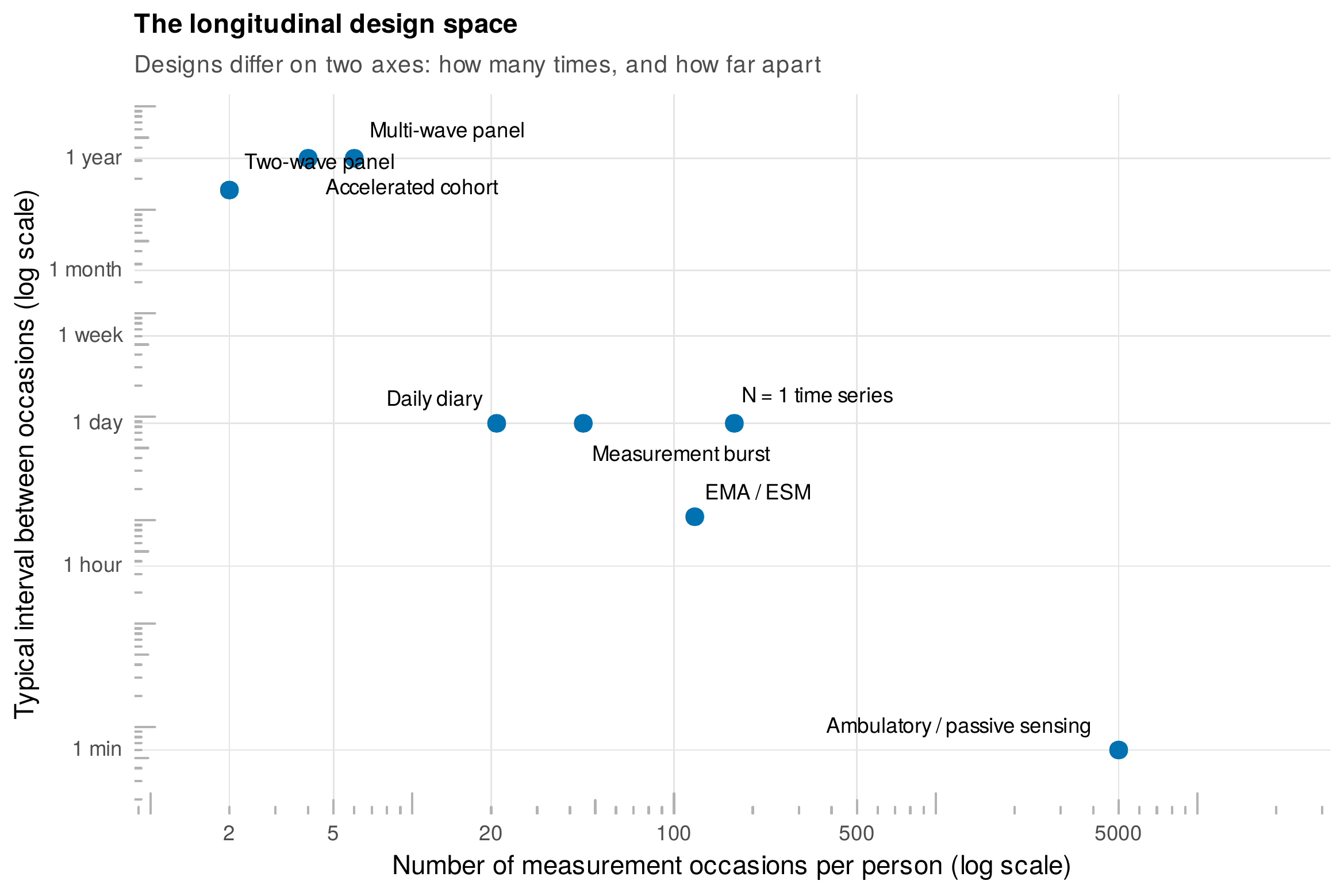
Note. Both axes are logarithmic. Named designs occupy overlapping regions rather than discrete points; a measurement-burst design (Section 2.4) deliberately combines a short interval within bursts and a long interval across them, and so cannot be placed at a single location.
Two orthogonal distinctions cut across this space and are worth fixing at the outset. The first is the distinction between a repeated cross-section, sometimes called a trend design, and a true panel. A repeated cross-section surveys a fresh sample of people on each occasion, so it can describe how a population average changes over time but can never observe an individual changing, because no individual appears twice. A true panel follows the same individuals across occasions and therefore carries within-person information. Only the panel can address the within-person questions of Chapter 1; a trend design, however many waves it has, remains a sequence of between-person snapshots. The second distinction is between prospective and retrospective measurement. A prospective design records states as they occur; a retrospective design asks people to recall states after the fact. Because memory reconstructs rather than replays, retrospective reports are subject to systematic recall biases that grow with the interval being recalled, and reducing this bias is one of the primary motivations for the intensive prospective designs treated later in this chapter (Shiffman, Stone, & Hufford, 2008).
2.2 Classical Panel and Cohort Designs
The oldest problem in longitudinal research is developmental, and it exposes a confound that no amount of data from a single design can resolve. Suppose we observe that fifty-year-olds score lower on a cognitive task than thirty-year-olds. Three explanations are entangled. The difference could reflect age, a genuine within-person change that comes with growing older. It could reflect cohort, a stable difference between people born in different eras who were educated and nourished differently. Or it could reflect period, an influence of the historical moment of measurement that affects everyone alike. Schaie (1965) organized these three influences into a framework whose logic still governs developmental design, shown in Figure 2.2. Each cell of the grid is a combination of a birth cohort and a measurement period, and the age in that cell is fixed by the other two. A cross-sectional study samples a single column, one period across several cohorts, and so confounds age with cohort. A single-cohort longitudinal study samples a single row, one cohort across several periods, and so confounds age with period. A cohort-sequential design samples many cohorts across many periods, the full grid, and only such a design offers any hope of separating the three.
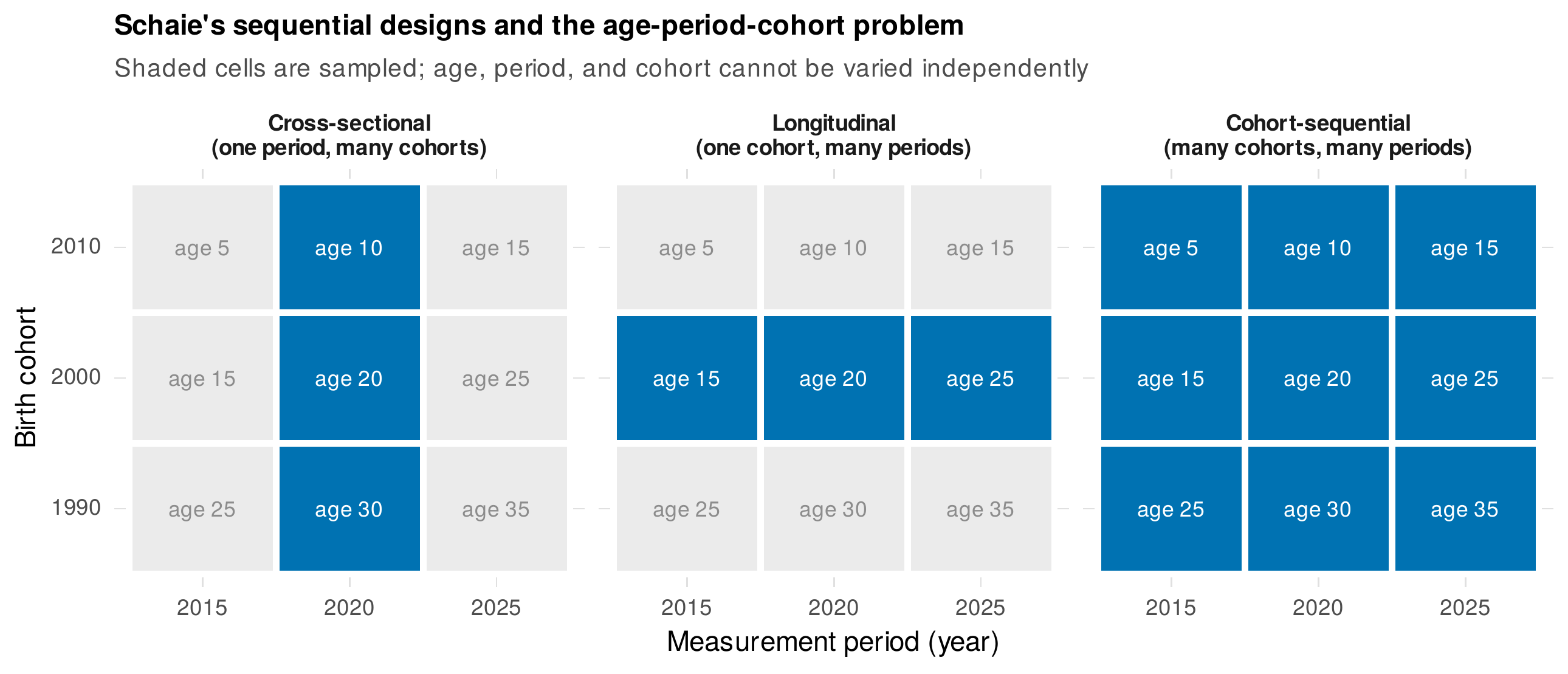
Note. Rows are birth cohorts, columns are measurement periods, and the label in each cell is the age at that combination. Shaded cells are sampled by each design. Because age equals period minus cohort, the three dimensions cannot be manipulated independently, and each single-slice design confounds two of them.
The reason the three influences cannot be separated by fiat is not statistical timidity but arithmetic, and it is worth seeing plainly.
Foundations Box • the age-period-cohort linear dependency
Let a person’s age at measurement be \(A\), the calendar period of measurement be \(P\), and the person’s birth cohort be \(C\). By definition, age is the elapsed time since birth, so
The three quantities are exactly linearly dependent: any one is determined by the other two. Now consider a model that tries to estimate a separate linear effect of each, \(\;y = \beta_0 + \beta_A A + \beta_P P + \beta_C C + \varepsilon\). Substituting Equation (2.1) shows that the trio \((\beta_A, \beta_P, \beta_C)\) can be shifted by any constant \(\delta\), replacing them with \((\beta_A + \delta,\; \beta_P - \delta,\; \beta_C + \delta)\), without changing a single fitted value. The linear components of age, period, and cohort are therefore not separately identified: infinitely many parameter sets fit the data equally well. No estimator, however sophisticated, can break this tie without an outside assumption (for example, that the period effect is null, or that two adjacent cohorts are equal). This is an identification problem, not a power problem, and collecting more data in the same design does not solve it.
The practical escape is the accelerated longitudinal design, also called a cohort-sequential or convergence design, illustrated in Figure 2.3 using the book’s school_growth data. Rather than following one cohort of children for the full six years from grade 3 to grade 8, which would take six years of funding and expose the study to six years of attrition, the design recruits three overlapping cohorts and follows each for four years. One cohort is observed in grades 3 through 6, a second in grades 4 through 7, and a third in grades 5 through 8. Stitched together, the cohorts span the entire grade 3 to grade 8 range in only four calendar years, and the overlap in grades 5 and 6, where all three cohorts are observed, provides the leverage to test whether the separate cohort trajectories align. The design buys time at the price of an assumption: that the shape of the age trajectory is the same across the overlapping cohorts, so that the pieces can be joined into one curve. That assumption is not free, but unlike the raw age-period-cohort tangle it is testable, precisely by checking whether the cohorts agree in their region of overlap (the modeling is developed in Chapter 14 and revisited for development in Chapter 34).
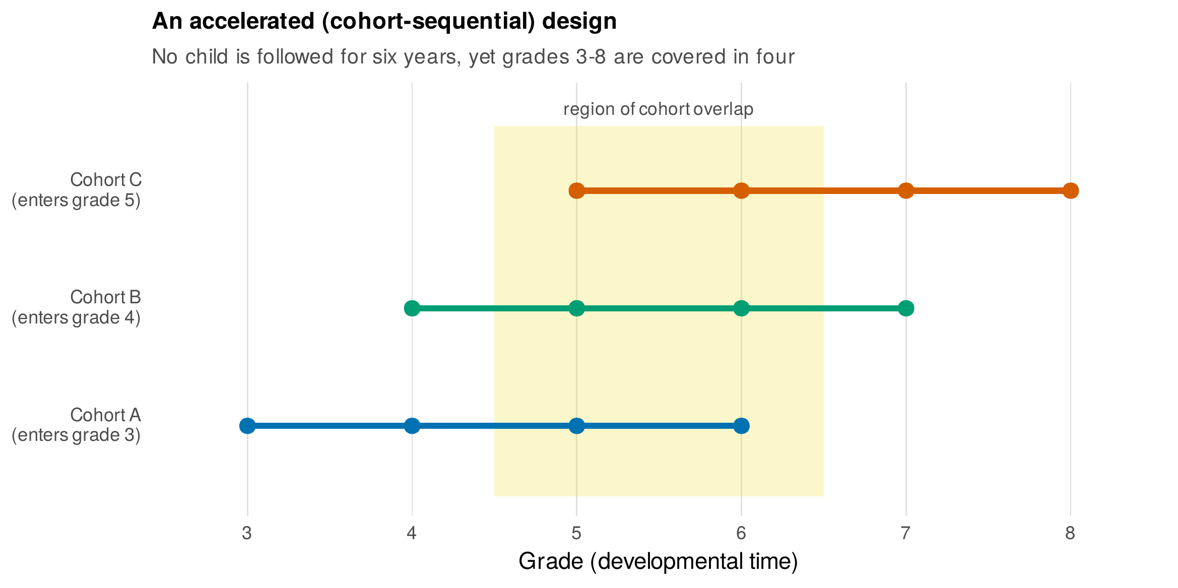
Note. Each horizontal segment is one cohort from school_growth, observed for four grades. The shaded band marks the grades where cohorts overlap; agreement among cohorts in this band is the testable assumption that licenses joining them into a single trajectory.
Panel designs of every length face a second family of design problems that concern who remains in the study and how measurement itself changes people. Attrition, the loss of participants over time, is the most consequential, because it is rarely random: those who drop out often differ systematically from those who remain, so that the surviving sample drifts away from the population of interest. The design responses are practical, including careful tracking protocols, incentives graduated to retention, and, in long panels, refreshment samples that add new participants to replace lost ones. Crucially, and as Chapter 6 develops at length, what matters for bias is not the raw attrition rate but the mechanism: attrition that depends only on previously observed values can be handled by modern estimators, whereas attrition that depends on the unobserved outcome itself cannot be fully corrected by any analysis. A second problem is the retest or practice effect, in which repeated exposure to the same instrument improves performance for reasons that have nothing to do with the construct, a serious confound for cognitive outcomes. Design remedies include parallel test forms, deliberate spacing of assessments, and, in the measurement-burst designs discussed below, using the first burst to absorb the steepest practice gains. A third and subtler problem is panel conditioning, in which the act of being repeatedly surveyed changes attitudes or behavior, so that seasoned panelists no longer respond as fresh respondents would.
2.3 Intensive Longitudinal Designs
The lower and right regions of the design space have been transformed over the past three decades by a family of designs that sample experience densely and in situ, as life is lived rather than as it is later recalled. These designs travel under an unfortunate profusion of names, and the first task is to disambiguate them, which Table 2.1 attempts. The daily diary samples once or a few times per day, typically for one to several weeks. The experience-sampling method and ecological momentary assessment sample more densely, several times per day, and emphasize momentary rather than daily states; the two terms arose in different literatures, personality and clinical-behavioral respectively, but now overlap almost completely (Csikszentmihalyi & Larson, 1987; Stone & Shiffman, 1994). Ambulatory assessment is the broadest term and explicitly includes physiological and behavioral channels such as ambulatory heart rate and actigraphy, not only self-report (Trull & Ebner-Priemer, 2013). Passive sensing, or digital phenotyping, collects data continuously from smartphone and wearable sensors with no active response from the participant at all (Harari et al., 2016; Mohr, Zhang, & Schueller, 2017). These are not competing labels for one thing; they mark real differences in density, in channel, and in participant burden.
Table 2.1. A terminology map for intensive longitudinal designs.
| Design | What it collects | Typical density | Channel |
|---|---|---|---|
| Daily diary | End-of-day reports of the day’s events, moods, behaviors | 1–3 per day, 1–4 weeks | Self-report |
| Experience sampling (ESM) | Momentary states at prompted moments | 3–10 per day, 1–2 weeks | Self-report |
| Ecological momentary assessment (EMA) | Momentary states, symptoms, behaviors (clinical origin) | 3–10 per day, 1–4 weeks | Self-report |
| Ambulatory assessment (AA) | Self-report plus physiology and movement | Varies; continuous for sensors | Self-report + sensor |
| Passive / digital phenotyping | Sensor and log data with no active response | Continuous | Sensor / device logs |
Note. Densities are typical rather than definitional; designs are frequently hybridized, for example a daily diary combined with a few random momentary prompts.
Within the self-report designs, the single most important design decision is the sampling scheme: the rule that determines when a prompt occurs. Wheeler and Reis (1991) drew the enduring three-way distinction, illustrated on a three-day strip in Figure 2.4. Interval-contingent sampling prompts on a fixed schedule, such as every evening at nine o’clock; it is simple and predictable but cannot capture events that fall between prompts and invites retrospection over the interval. Signal-contingent sampling prompts at random times, usually one random moment within each of several equal blocks of the waking day, which minimizes anticipation and gives an approximately representative sample of moments; it is the default for studies of momentary states such as affect. Event-contingent sampling asks the participant to report whenever a defined event occurs, such as a social interaction, a cigarette, or a panic attack; it is the only scheme that reliably captures rare or bounded events, but it depends entirely on the participant recognizing and recording the event. The schemes are not mutually exclusive, and hybrid designs that combine, say, signal-contingent mood prompts with event-contingent reports of conflict are common. Table 2.2 gives guidance for matching scheme to question.
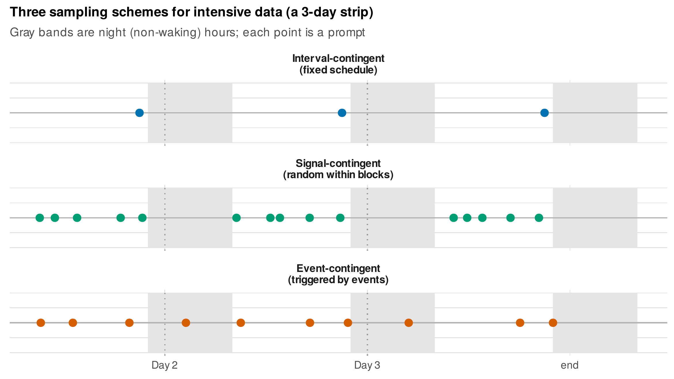
Note. Gray bands mark night (non-waking) hours; each point is a prompt. Interval-contingent prompts fall on a fixed schedule, signal-contingent prompts fall at random moments within equal blocks of the waking day, and event-contingent prompts fall whenever a defined event occurs.
Table 2.2. Selecting a sampling scheme.
| If the question concerns... | Prefer... | Rationale |
|---|---|---|
| Average momentary states and their moment-to-moment dynamics | Signal-contingent | A representative sample of unanticipated moments; supports lagged within-person models |
| Regular daily rhythms or end-of-day summaries | Interval-contingent | Fixed timing aligns reports to a natural cycle; lower burden |
| Rare, bounded, or self-defining events (conflicts, lapses, panic) | Event-contingent | Only scheme that captures events reliably; avoids diluting the sample with irrelevant moments |
| Both states and events | Hybrid | Signal-contingent backbone with event-triggered reports layered on |
Note. Base rate of the target is decisive: the rarer and more bounded the phenomenon, the stronger the case for event-contingent capture.
Once a scheme is chosen, a protocol is specified by a handful of design parameters, and it is here that intensive designs succeed or fail as practical instruments. Table 2.3 lists the parameters with recommended ranges. The central tension among them is the burden-compliance trade-off, sketched in Figure 2.5: every additional prompt per day, every additional item per prompt, and every additional week of the study raises respondent burden and lowers compliance, the proportion of scheduled prompts actually answered. The trade-off is not merely a nuisance to be minimized, because compliance interacts with missingness: if the least compliant participants are also the most symptomatic, low compliance becomes a missing-data mechanism that biases estimates (Chapter 6). The historical benchmark for why prospective electronic capture matters is Stone, Shiffman, Schwartz, Broderick, and Hufford (2002), who compared paper diaries carrying hidden timestamps against electronic diaries and found that participants frequently completed paper diaries in batches, backfilling or forward-filling entries, while reporting near-perfect compliance; reported compliance was about 90 percent, but actual compliance inferred from the timestamps was closer to 11 percent. The lesson is that compliance must be measured, through timestamps and completion logs, not assumed from self-report, and that design choices, shorter items, brief training, well-timed reminders, and appropriate incentives, shift the entire compliance curve upward rather than merely trading one prompt for another.
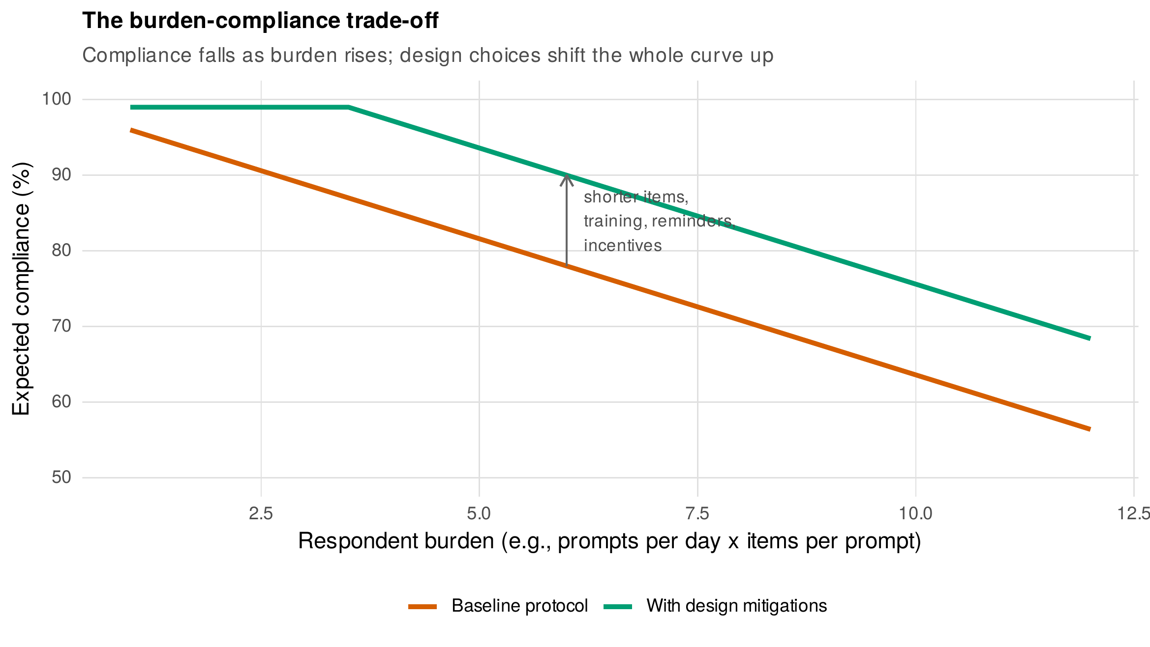
Note. Stylized illustration. Compliance declines as respondent burden rises; design mitigations such as shorter items, training, reminders, and incentives raise the entire curve rather than changing its slope. The vertical arrow marks the compliance gain achievable at a fixed level of burden.
Table 2.3. A design-parameter checklist for intensive longitudinal protocols.
| Parameter | Typical range | Consideration |
|---|---|---|
| Study duration | 7–28 days | Long enough for the target dynamics; short enough to sustain compliance |
| Prompts per day | 3–10 | More prompts resolve faster dynamics but raise burden and reactivity |
| Response window | 10–30 minutes | Short enough to keep reports momentary; long enough to be answerable |
| Items per prompt | 5–15 | The chief lever on per-prompt burden; protect it fiercely |
| Training session | 1 in-person or guided | Reduces early dropout and item misunderstanding |
| Reminders | Escalating, non-punitive | Improve compliance without inducing reactance |
| Incentives | Graduated or completion-based | Reward sustained compliance, not only enrollment |
| Compliance target | \(\geq 80\%\) answered | State it in advance; monitor it live; report it honestly |
Note. Ranges are conventional starting points, not rules; the defensible values follow from the estimand and are best confirmed by the simulation-based planning of Chapter 4.
In Practice • evaluating an experience-sampling platform
Software for delivering prompts and capturing responses dates quickly, so evaluate platforms by capability rather than brand. A serviceable platform should: deliver all three sampling schemes and hybrids; timestamp every prompt and every response, storing the delay between them; support flexible prompt windows and escalating reminders; branch items conditionally (so a follow-up appears only when relevant); operate offline and synchronize later; export raw, timestamped data in an open format; and meet the security and consent requirements of momentary data, including encryption and, where sensitive items are used, a mechanism for risk response (see the ethics box in Section 2.6). Name categories of capability in your protocol, not a product, so that the protocol survives the next change of vendor.
2.4 Timescale Matching and Measurement Bursts
Chapter 1 warned that a process has a timescale and a design has a timescale, and that a mismatch can manufacture apparent trends where none exist, the aliasing problem of Figure 1.4. Design is where that warning is acted upon. The sampling density must be fast enough to resolve the dynamics of interest: a process that fluctuates within a day cannot be recovered by daily sampling, just as a melody cannot be reconstructed from one note per measure. But faster is not simply better, because denser sampling raises burden and reactivity and, for slowly moving constructs, wastes effort resolving variation that is not there. The design task is to match, not to maximize.
The measurement-burst design, whose logic Nesselroade (1991) captured in the image of development as a fabric woven from a slowly changing warp and a rapidly fluctuating weft, resolves a genuine dilemma: how to study both fast within-person dynamics and slow developmental change in one study. The solution, illustrated in Figure 2.6, is to embed short bursts of intensive sampling within a long-term panel. Each burst, perhaps a week of several daily prompts, characterizes the person’s current dynamics and variability; the bursts are repeated at long intervals, perhaps annually, so that change in those dynamics can itself be tracked across development (Sliwinski, 2008). What a burst design uniquely estimates is therefore not level or trend alone but the developmental trajectory of within-person variability and dynamics, quantities invisible to either a sparse panel or a single intensive burst. The cost is again an interval-dependence caution: because estimated dynamic quantities such as lagged effects depend on the spacing between observations, the within-burst schedule must be held constant across bursts, or the continuous-time methods of Chapter 27 must be used to make bursts comparable.
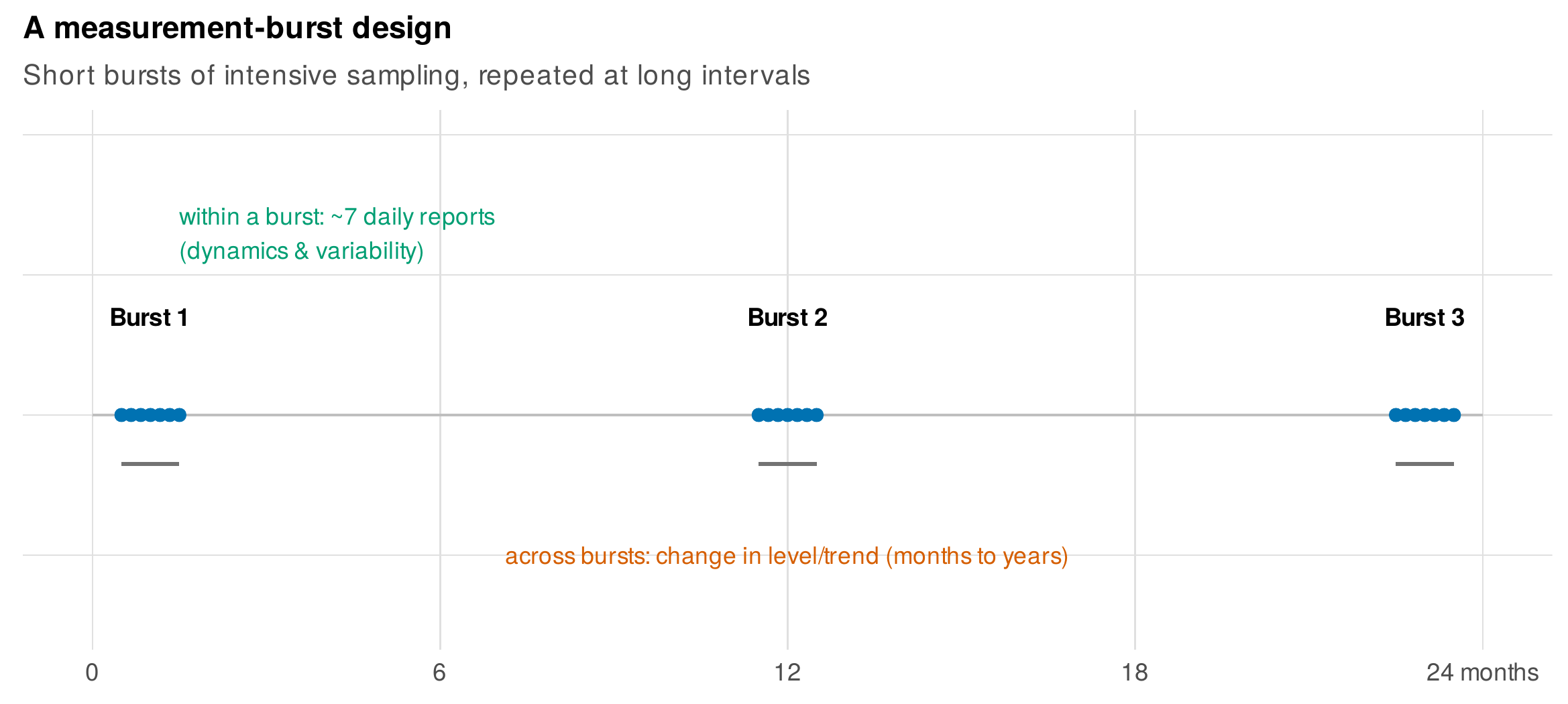
Note. Each cluster is a burst of closely spaced daily reports; bursts recur at long intervals. Within-burst spacing estimates dynamics and variability; the spacing across bursts estimates how those quantities change over months and years.
2.5 Designs for Intervention Research Over Time
Repeated measurement is also the backbone of intervention research, where the design question becomes how to arrange treatment and assessment in time so that a causal effect on the trajectory is estimable. The familiar case is the randomized controlled trial with repeated outcomes, exemplified by the book’s therapy_rct data, in which patients are randomized to arms and then assessed repeatedly, here on a depression scale across twelve weekly visits, so that the arms’ trajectories, not merely their endpoints, can be compared (Chapters 10 through 13). Two features of such trials are themselves design problems treated later: differential dropout across arms, which therapy_rct builds in deliberately (Chapter 6), and the timing of events such as relapse, which calls for the survival methods of Chapter 29. The stepped-wedge trial, in which clusters cross from control to intervention at randomly ordered times, and the interrupted time series, in which a single unit is observed densely before and after an intervention (Chapter 24), extend the same logic to settings where simultaneous randomization is impractical.
A newer design has emerged specifically for interventions delivered through mobile devices, where the question is not whether a treatment works on average but whether a particular prompt, delivered at a particular moment, helps in the moments that follow. The micro-randomized trial, illustrated in Figure 2.7, randomizes at the level of the decision point rather than the person: at each of many moments across the study, the participant is randomly assigned to receive an intervention prompt or not, and a proximal outcome is measured shortly afterward (Klasnja et al., 2015). Because randomization is repeated within each person hundreds of times, the design estimates time-varying and context-dependent effects of the momentary intervention, which is exactly what is needed to build a just-in-time adaptive intervention, a treatment that decides what to deliver, and when, from the person’s current state (Nahum-Shani et al., 2018). The analysis of such trials is previewed in Chapter 33.
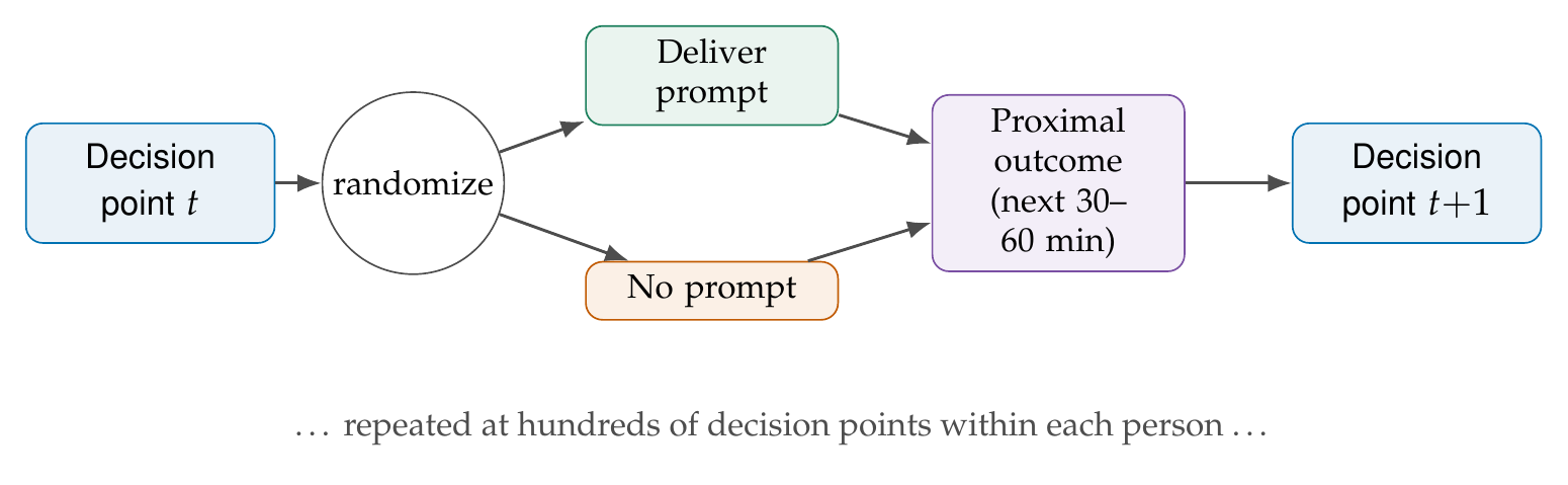
Note. At each decision point the participant is randomized to receive an intervention prompt or not, and a proximal outcome is measured shortly afterward. Repetition within person supports estimation of time-varying, context-dependent momentary effects.
2.6 Validity Threats Specific to Repeated Measurement
Measuring people repeatedly introduces threats to validity that single-occasion studies never face, and a competent design anticipates them. The first is reactivity: the act of self-monitoring can change the very behavior being monitored, as when tracking one’s mood or smoking alters mood or smoking. The evidence is that such effects are generally modest but genuinely domain-dependent, larger for behaviors under deliberate control and for participants motivated to change, so reactivity should be assessed rather than assumed away, for example by comparing early and late reports or by staggering the onset of monitoring. The second is the retest effect already noted for cognitive outcomes. A third, peculiar to high-frequency designs, is item-order and context effects: at many repetitions, the order of items and the immediate context of a prompt can shape responses, which argues for randomizing item order and keeping the momentary context in the record. A fourth is careless responding under sustained burden, in which fatigued participants answer without attending; its detection, through response times, straight-lining, and embedded checks, is treated in Chapter 5. Table 2.4 pairs these threats with design countermeasures.
Table 2.4. Validity threats specific to repeated measurement, with design countermeasures.
| Threat | What it does | Design countermeasure |
|---|---|---|
| Reactivity / reflexivity | Monitoring changes the monitored behavior | Assess early vs. late; staggered onset; a monitoring-only baseline |
| Retest / practice | Repeated exposure inflates performance | Parallel forms; spacing; absorb practice in a first burst |
| Panel conditioning | Repeated surveying changes attitudes | Refreshment samples; rotate items; limit tenure |
| Item-order / context effects | Response depends on order and situation | Randomize item order; record context; fixed core items |
| Careless responding | Fatigue degrades data quality | Short prompts; attention checks; response-time screening (Ch. 5) |
| Selective attrition | Dropout depends on the outcome | Tracking; incentives to retention; plan for MAR/MNAR (Ch. 6) |
Note. Countermeasures are design-side; their analytic complements (missing-data models, careless-response detection) appear in the referenced chapters.
Two further threats are less about measurement error than about whom the study represents and what duty it incurs. Selection and generalizability deserve explicit attention because intensive designs recruit a particular kind of participant: those who own a suitable device, tolerate frequent interruption, and consent to dense observation of their lives. Findings from such samples may not generalize to those who decline, and the design should document coverage and consent rates rather than treat the enrolled sample as the population. Finally, momentary data are ethically weighty in a way that occasional surveys are not, because dense records of location, behavior, and mood can re-identify and expose participants, and because momentary assessment of sensitive states carries a duty of care.
Ethics Box • monitoring momentary suicidality
Studies of self-harm and suicidality increasingly assess these states momentarily, which raises an acute design question: what happens when a participant, alone with a phone, reports imminent risk? A defensible protocol decides this in advance, not in the moment. Concretely, such a protocol specifies a risk item with a validated threshold; an automated, immediate on-screen response when the threshold is crossed, providing crisis resources and, where consented, a pathway to contact; a monitoring plan under which flagged responses are reviewed on a stated schedule by a qualified clinician, with the review latency disclosed to participants so that no one mistakes the study for an emergency service; a pre-specified escalation and duty-to-warn procedure consistent with local law and IRB approval; and informed consent that states plainly what will and will not happen if risk is reported. The design principle is that a study which asks about risk assumes responsibility for a response, and that responsibility must be engineered into the protocol before the first prompt is sent.
Common Pitfall • “sampling faster is always better”
The intuition that more data can only help fails for intensive designs in three distinct ways. First, burden: each added prompt lowers compliance and can convert a study’s most informative participants into its most missing (Figure 2.5). Second, reactivity: very frequent prompting can itself change the behavior under study, so that the measurement distorts the phenomenon. Third, and least obvious, aliasing in reverse: sampling a slow construct very fast does not sharpen it but merely spends burden resolving noise, while sampling a fast construct too slowly, the classic aliasing of Chapter 1, misrepresents it entirely. The correct target is not the highest feasible density but the density matched to the timescale of the process, confirmed where possible by the simulation-based planning of Chapter 4.
2.7 Choosing a Design: Three Worked Decisions
Design principles are best seen at work. Consider three studies, each beginning from a question and ending in a defensible specification, summarized in Table 2.5. The first asks whether daily stress disturbs that night’s sleep, a within-person question about a process that unfolds over hours to a day. Because the coupling of interest is daily and the constructs are momentary states rather than rare events, a signal-contingent or interval-contingent daily diary of about fourteen days, with an evening sleep report and several daytime stress prompts, is appropriate; two waves would not resolve the daily coupling, and second-by-second sensing would be overkill. The second asks how emotional reactivity to stressors changes across adolescence, a question about the developmental trajectory of a within-person dynamic, which is exactly what a measurement-burst design exists to answer: a week-long signal-contingent burst repeated annually across the adolescent years, so that reactivity estimated within each burst can be tracked across bursts. The third asks what momentary states forecast a lapse in the days after addiction treatment, a question about a rare, bounded, and clinically urgent event, which argues for a hybrid scheme, a signal-contingent backbone to characterize states plus event-contingent reports at each lapse, delivered by a platform with a risk-response protocol. These three vignettes return in Chapter 4, where each is carried through a formal power and precision analysis.
Table 2.5. Three worked design specifications.
| Stress and sleep | Adolescent reactivity | Post-treatment lapse | |
|---|---|---|---|
| Question family | Within-person dynamics (daily) | Change in dynamics (developmental) | Dynamics + event timing |
| Design | Daily diary | Measurement burst | Hybrid EMA |
| Scheme | Signal + evening interval | Signal-contingent bursts | Signal + event-contingent |
| Duration | 14 days | 1-week bursts, yearly | 21 days post-discharge |
| Prompts/day | 5 + 1 evening | 6 within burst | 5 + event triggers |
| Key threat | Reactivity of self-monitoring | Retest across bursts | Attrition; risk of harm |
Note. Each specification is developed into a powered protocol in Chapter 4. Prompt counts are starting points to be confirmed by simulation.
To make a protocol concrete, Figure 2.8 shows two participant-facing prompt screens for the book’s affect_ema study, whose full protocol is a fourteen-day, six-prompt signal-contingent design with a fifteen-minute response window and a short momentary item set covering stress, negative and positive affect, and social context. Seeing the actual screens is a useful discipline, because the item wording, the response scale, and the number of taps required are precisely the design details that determine burden and data quality, and they are easy to neglect when a protocol exists only as prose.
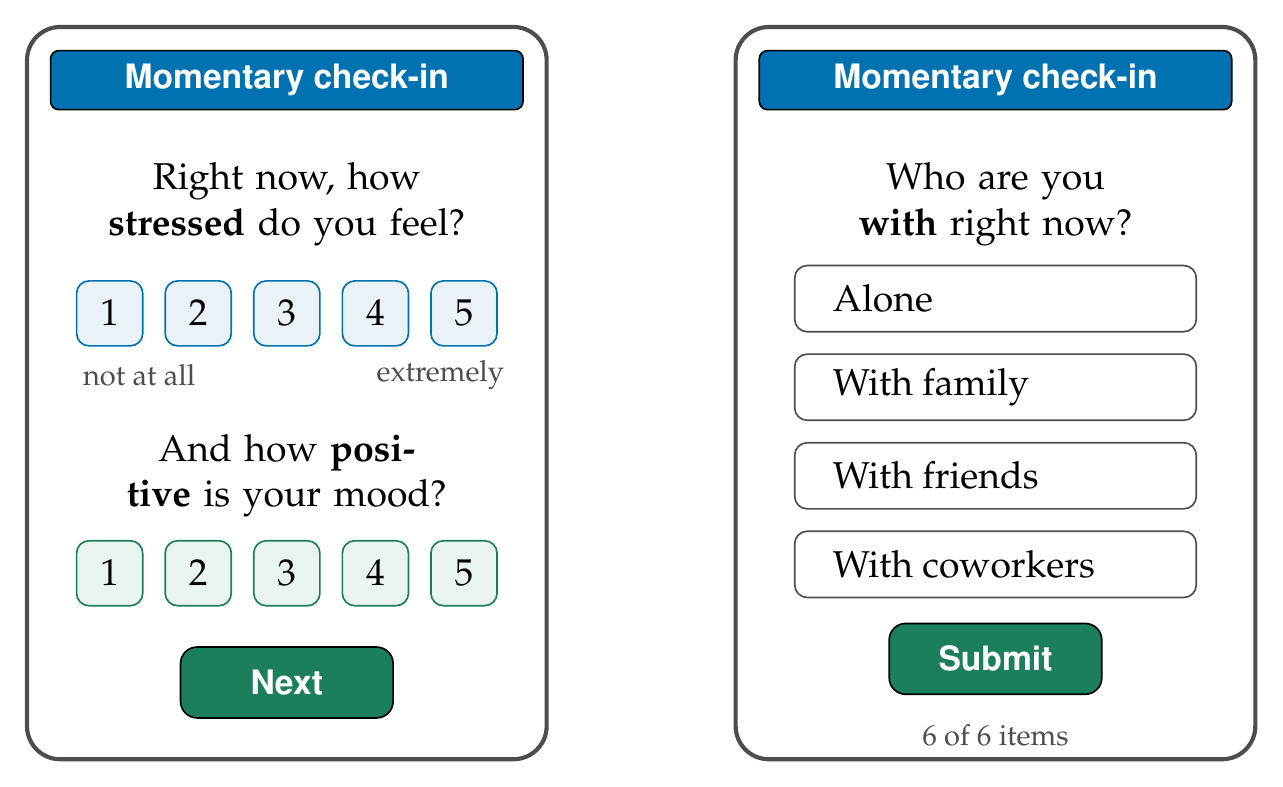
affect_ema protocol.Note. Mock-ups, not screenshots. Item wording, response-scale granularity, and the number of taps per prompt are design decisions that directly determine respondent burden and data quality.
2.8 Building a Sampling Schedule in R
A design becomes real when it is turned into a concrete schedule of prompts and a concrete data structure. This section shows both, using only base R so that the logic is transparent. The first task is to generate a signal-contingent schedule: for each study day, one random prompt time is drawn within each of several equal blocks of the waking day, which is the scheme underlying Figure 2.4 and the affect_ema protocol. The companion function is shipped in the Examples scripts; its core is short.
# Signal-contingent schedule: n_blocks random prompts per day,
# one within each equal block of the waking window, with a minimum
# separation so two prompts never crowd together.
make_schedule <- function(n_days = 14, n_blocks = 6,
                          wake = c(9, 22), min_gap = 0.75, seed = 1) {
  set.seed(seed)
  edges <- seq(wake[1], wake[2], length.out = n_blocks + 1)
  out <- data.frame()
  for (d in seq_len(n_days)) {
    repeat {
      times <- mapply(function(lo, hi) runif(1, lo, hi),
                      edges[-(n_blocks + 1)], edges[-1])
      if (all(diff(sort(times)) >= min_gap)) break   # enforce spacing
    }
    out <- rbind(out, data.frame(day = d, block = seq_len(n_blocks),
                                 prompt_hour = round(sort(times), 2)))
  }
  out
}

sched <- make_schedule(n_days = 14, n_blocks = 6, seed = 2026)
head(sched, 6)
nrow(sched)                       # 84 scheduled prompts over 14 days
The second task is to look at a longitudinal dataset as a design object before any model is fitted, which for a trial means checking the arms, the assessment schedule, and the pattern of dropout. Using therapy_rct, we confirm the balance of the two arms, count the weekly assessments, and, most importantly for design, tabulate how many patients remain observed at each week, because the shape of that curve is the study’s attrition profile.
therapy_rct <- readRDS("Examples/data/therapy_rct.rds")

table(therapy_rct$arm[therapy_rct$week == 0])      # 120 Treatment, 120 Control
length(unique(therapy_rct$week))                   # 12 weekly assessments

# Attrition profile: number still observed (hdrs not missing) each week
observed_by_week <- tapply(!is.na(therapy_rct$hdrs),
                           therapy_rct$week, sum)
round(observed_by_week / 240 * 100)                # percent retained per week
Running this shows the retained fraction declining from 100 percent at baseline to roughly half by the final week, and because the dropout in these data was generated to depend on patients’ own worsening scores, it is a concrete instance of the attrition-as-mechanism problem: the patients who leave are not a random subset, so the observed sample at week 11 is healthier than the randomized sample at week 0. That is a design fact to be confronted in the analysis (Chapter 6), and seeing it in the retention curve at the design stage is exactly the habit this section is meant to instill.
2.9 Writing the Method Section for a Longitudinal Design
A longitudinal design is only as credible as its reporting, and reviewers of intensive and panel studies now expect specific details that authors of cross-sectional work never had to provide. The design counterpart of Chapter 1’s advice on writing results is a short discipline for the Method section, organized around four commitments. First, report the design in the two coordinates of Figure 2.1: state the number of intended occasions and their spacing explicitly, for example “participants completed six signal-contingent prompts per day for fourteen consecutive days,” rather than the uninformative “participants completed a diary study.” Second, report the sampling scheme and its parameters: the contingency type, the blocking of the day, the response window, the item budget per prompt, and the reminder and incentive structure, so that another team could reproduce the protocol. Third, report compliance as measured, not as intended: give the achieved compliance rate computed from timestamps, its distribution across participants, and the rule used to retain or exclude low-compliance cases, because an unstated compliance rate is now read as a red flag rather than a courtesy. Fourth, report attrition and its handling: the number and timing of dropouts, any analysis comparing completers with non-completers, and the planned missing-data approach, since, as this chapter has stressed, the mechanism of missingness rather than its rate is what threatens validity.
A model paragraph, drawing these commitments together for the affect_ema protocol, reads: “One hundred twenty adults completed a fourteen-day experience-sampling protocol. Using a signal-contingent scheme, the mobile application delivered six prompts per day at random times within six equal blocks of the waking day (approximately 9:00 to 22:00), each with a fifteen-minute response window. Each prompt comprised eight items assessing momentary stress, negative and positive affect, and social context. Participants completed a brief training session and received graduated compliance-based incentives. The achieved compliance rate, computed from response timestamps, was 73 percent (SD across participants reported in Table X); missingness was more frequent following high-stress prompts, consistent with a missing-at-random mechanism, and was handled with full-information maximum likelihood (Chapter 6).” Every clause of that paragraph is a design decision made earlier in this chapter, which is the point: the Method section is where the design, well made, pays off as credibility.
Software Note • the companion design tools
The Examples folder ships the scheduling function make_schedule() used above, together with the seeded generators for the book’s design-relevant datasets: school_growth for the accelerated-cohort example of Figure 2.3, and therapy_rct for the trial example, including its built-in monotone missing-at-random dropout and post-treatment relapse times for the survival analysis of Chapter 29. Each dataset carries a codebook documenting its design and its data-generating process, so that the design ideas of this chapter can be inspected in data as well as read about.
2.10 Common Misconceptions
Four beliefs recur and mislead. First, that ecological momentary assessment is just a diary done more often: this misses the logic of sampling schemes and the recall-bias rationale that motivates momentary capture, treating a design choice as a mere frequency knob (Shiffman, Stone, & Hufford, 2008). Second, that attrition matters only if its rate exceeds some threshold: as Chapter 6 shows, a low rate of outcome-dependent dropout can bias estimates more than a high rate of random dropout, because it is the mechanism, not the percentage, that governs bias. Third, that accelerated designs assume nothing: they trade six years for four only by assuming that the age trajectory is cohort-invariant in the region of overlap, an assumption that must be stated and tested rather than presumed. Fourth, and most consequential in practice, the question “how many days and beeps do I need?” has no context-free answer: the required density and duration depend on the estimand, whether a mean, a trend, a variance, or a lagged coefficient, and are best resolved by the simulation-based power analysis of Chapter 4 rather than by rules of thumb.
Chapter Summary
Design fixes what analysis can later recover. Every repeated-measures study occupies a position in a space defined by the number of occasions and their spacing (Figure 2.1), and the first design distinctions, trend versus panel and prospective versus retrospective, determine whether within-person questions are answerable at all. Developmental designs confront the age-period-cohort identification problem, an arithmetic tangle (Equation 2.1) that no single-slice design can undo and that accelerated designs escape only by a testable cohort-invariance assumption. Intensive designs are organized by their sampling scheme, interval-, signal-, or event-contingent, and are governed by the burden-compliance trade-off, which makes measured compliance and honest attrition reporting central. Measurement bursts marry fast and slow timescales; micro-randomized trials randomize the moment rather than the person. Repeated measurement carries its own validity threats, from reactivity to selective attrition, and, for sensitive momentary data, a duty of care that must be engineered into the protocol. The chapter closed with three worked design decisions, a schedule-building tool in R, and a discipline for reporting a longitudinal design.
Where to Go Next
The next chapters follow the data these designs produce: Chapter 3 asks whether a construct measured repeatedly means the same thing at each occasion; Chapter 4 turns each design decision into a quantitative question of power and precision, carrying forward the three worked vignettes; Chapter 5 addresses the management of the multi-stream data these protocols generate; and Chapter 6 confronts the missingness that attrition and imperfect compliance leave behind. The thread from Chapter 1 continues here: a design is a commitment about whose variance, and over what timescale, a study will be able to speak.
Exercises
- 2.1 Critique a protocol. Obtain the methods section of a published experience-sampling study and evaluate it against the design-parameter checklist of Table 2.3. Which parameters are reported, which are missing, and what could a reader not reproduce?
- 2.2 Choose a scheme. You wish to study the antecedents of binge-drinking episodes in undergraduates. Specify a sampling scheme, justify the choice of event- versus signal-contingent (or a hybrid), and state how you would define and detect the target event.
- 2.3 Sketch an accelerated design. With three years of funding, design a study spanning ages 10 to 18. Specify the cohorts and their overlap, draw the coverage plot in the style of Figure 2.3, and state the assumption your design requires.
- 2.4 Diagnose the confound. Read a provided abstract that claims an age effect from cross-sectional data. Identify the age-period-cohort confound precisely, and describe the design that would be needed to support the causal claim.
- 2.5 Draft an ethics protocol. Write the risk-response paragraph for a study that assesses momentary suicidal ideation, following the ethics box of Section 2.6. Specify the threshold, the automated response, the review latency, and the escalation procedure.
- 2.6 Build a schedule. Using
make_schedule()from theExamplesscripts, generate a signal-contingent schedule of five prompts per day for ten days, and plot the prompt times in the style of Figure 2.4. Verify that no two prompts fall within your minimum gap.
References
Baltes, P. B. (1968). Longitudinal and cross-sectional sequences in the study of age and generation effects. Human Development, 11(3), 145–171.
Bolger, N., Davis, A., & Rafaeli, E. (2003). Diary methods: Capturing life as it is lived. Annual Review of Psychology, 54, 579–616. https://doi.org/10.1146/annurev.psych.54.101601.145030
Bolger, N., & Laurenceau, J.-P. (2013). Intensive longitudinal methods: An introduction to diary and experience sampling research. Guilford Press.
Csikszentmihalyi, M., & Larson, R. (1987). Validity and reliability of the Experience-Sampling Method. The Journal of Nervous and Mental Disease, 175(9), 526–536. https://doi.org/10.1097/00005053-198709000-00004
Harari, G. M., Lane, N. D., Wang, R., Crosier, B. S., Campbell, A. T., & Gosling, S. D. (2016). Using smartphones to collect behavioral data in psychological science: Opportunities, practical considerations, and challenges. Perspectives on Psychological Science, 11(6), 838–854. https://doi.org/10.1177/1745691616650285
Kirtley, O. J., Lafit, G., Achterhof, R., Hiekkaranta, A. P., & Myin-Germeys, I. (2021). Making the black box transparent: A template and tutorial for registration of studies using experience-sampling methods. Advances in Methods and Practices in Psychological Science, 4(1). https://doi.org/10.1177/2515245920924686
Klasnja, P., Hekler, E. B., Shiffman, S., Boruvka, A., Almirall, D., Tewari, A., & Murphy, S. A. (2015). Microrandomized trials: An experimental design for developing just-in-time adaptive interventions. Health Psychology, 34(Suppl.), 1220–1228. https://doi.org/10.1037/hea0000305
Mehl, M. R., & Conner, T. S. (Eds.). (2012). Handbook of research methods for studying daily life. Guilford Press.
Mohr, D. C., Zhang, M., & Schueller, S. M. (2017). Personal sensing: Understanding mental health using ubiquitous sensors and machine learning. Annual Review of Clinical Psychology, 13, 23–47. https://doi.org/10.1146/annurev-clinpsy-032816-044949
Myin-Germeys, I., & Kuppens, P. (Eds.). (2021). The open handbook of experience sampling methodology: A step-by-step guide to designing, conducting, and analyzing ESM studies (2nd ed.). Center for Research on Experience Sampling and Ambulatory Methods Leuven.
Nahum-Shani, I., Smith, S. N., Spring, B. J., Collins, L. M., Witkiewitz, K., Tewari, A., & Murphy, S. A. (2018). Just-in-time adaptive interventions (JITAIs) in mobile health: Key components and design principles for ongoing health behavior support. Annals of Behavioral Medicine, 52(6), 446–462. https://doi.org/10.1007/s12160-016-9830-8
Nesselroade, J. R. (1991). The warp and woof of the developmental fabric. In R. M. Downs, L. S. Liben, & D. S. Palermo (Eds.), Visions of aesthetics, the environment, and development: The legacy of Joachim F. Wohlwill (pp. 213–240). Lawrence Erlbaum Associates.
Schaie, K. W. (1965). A general model for the study of developmental problems. Psychological Bulletin, 64(2), 92–107.
Shiffman, S., Stone, A. A., & Hufford, M. R. (2008). Ecological momentary assessment. Annual Review of Clinical Psychology, 4, 1–32. https://doi.org/10.1146/annurev.clinpsy.3.022806.091415
Sliwinski, M. J. (2008). Measurement-burst designs for social health research. Social and Personality Psychology Compass, 2(1), 245–261. https://doi.org/10.1111/j.1751-9004.2007.00043.x
Stone, A. A., & Shiffman, S. (1994). Ecological momentary assessment (EMA) in behavioral medicine. Annals of Behavioral Medicine, 16(3), 199–202. https://doi.org/10.1093/abm/16.3.199
Stone, A. A., Shiffman, S., Schwartz, J. E., Broderick, J. E., & Hufford, M. R. (2002). Patient non-compliance with paper diaries. BMJ, 324(7347), 1193–1194. https://doi.org/10.1136/bmj.324.7347.1193
Trull, T. J., & Ebner-Priemer, U. (2013). Ambulatory assessment. Annual Review of Clinical Psychology, 9, 151–176. https://doi.org/10.1146/annurev-clinpsy-050212-185510
Wheeler, L., & Reis, H. T. (1991). Self-recording of everyday life events: Origins, types, and uses. Journal of Personality, 59(3), 339–354. https://doi.org/10.1111/j.1467-6494.1991.tb00252.x