Chapter 36
The Complete Workflow: Method Selection, Reproducibility, and Reporting
The first chapter made a promise: that questions about change come in families, that the family determines the method, and that a reader who learns to name the question can be routed to the right analysis. This last chapter audits that promise. It consolidates the routing devices scattered through the book into one decision system, it codifies the reproducibility practices that turn a one-time analysis into a result another person can rebuild, it harmonizes the reporting checklists that accumulated chapter by chapter into a single standard, it formalizes the sensitivity doctrine that ran through every methods chapter as a running insistence, and it treats preregistration for longitudinal and intensive-longitudinal research at the working depth its timelines demand. The chapter is not a compliance sermon. Every standard it raises is shown paying off in a single end-to-end exemplar, a compact study taken from a question through its routing, its preregistration, its pipeline, its primary analysis, its sensitivity portfolio, its reporting audit, and its public repository, with the reasoning at each step tied back to the chapter that supplied it. The bookend structure is deliberate: Chapter 1 opened the map before any method existed, and this chapter revisits the same map now that all of them do, so that the reader who began by not knowing which method to use ends by knowing not only how to choose one but how to defend the choice, run it reproducibly, and report it so that a stranger, years later, can see exactly what was done and do it again. The closing image the book intends is simple: the reader can do this.
Learning Objectives
After working through this chapter, you should be able to: (1) use a master decision system, crossing the question family with the data structure and the assumptions you can defend, to justify a primary analysis, its mandatory sensitivity set, and the ceiling on what may be claimed; (2) build a reproducible longitudinal project, with immutable raw data, a locked package environment, a managed pipeline, a seed registry, and archived code and data; (3) apply the harmonized reporting checklist and know the items reviewers now expect for each model family; (4) design a sensitivity portfolio from the fork registry, run it as a multiverse, and report which forks move the conclusion as the finding it is; (5) preregister a longitudinal or experience-sampling study, including the decision-tree strategies that honest model-building requires, and report deviations; and (6) write longitudinal results estimand-first, with disciplined uncertainty language, and archive intensive data with its re-identification risks addressed.
36.1 The Master Decision System
The routing that Chapter 1 introduced as a single figure can now be stated as a system with three inputs and three outputs. The inputs are the question family, one of the five the book has used throughout, the data structure, described by the number of occasions per person, the number of persons, the regularity of the timing, and the type of the outcome, and the assumption budget, the set of assumptions the design and data let you defend, about the missingness mechanism, the invariance of measurement, the stationarity of dynamics, and the interval meaning of the scale. The outputs are the primary analysis that the inputs imply, the mandatory sensitivity analyses that the primary’s assumptions require, and the ceiling on the claims the design can support. Figure 36.1 is the full map, the counterpart of Figure 1.5, now populated with every method the book has developed and closed at the bottom by the workflow spine that this chapter formalizes. Table 36.1 is the companion that most students need first, because the hardest step is not choosing a method once the question is named but phrasing the question so that its estimand is unambiguous.
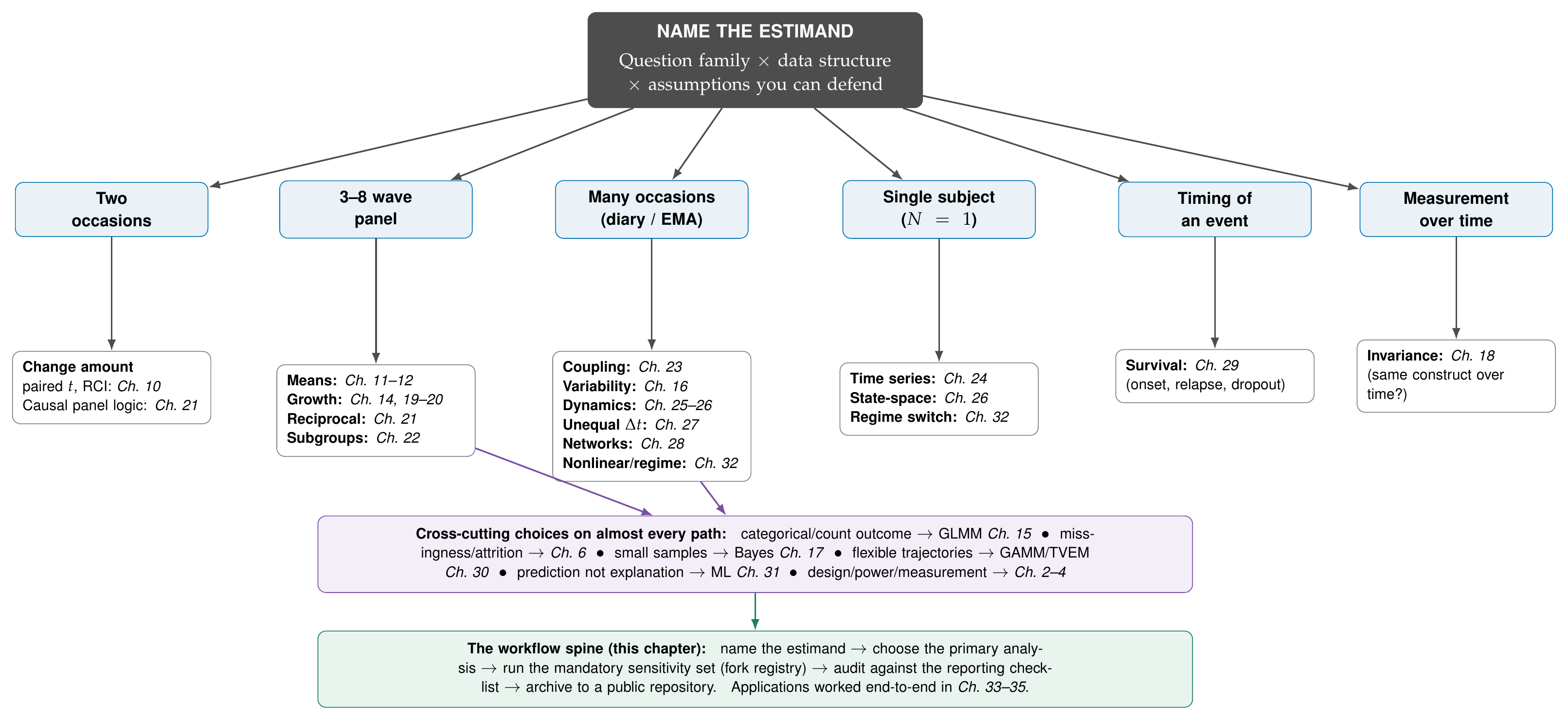
Note. Enter at the top by naming the estimand, follow the data structure to its category, and read the leaf for the methods that answer each question family, now including the flexible, dynamic, and nonlinear tools developed after Chapter 1. The purple band lists the cross-cutting choices; the green band adds the workflow spine this chapter formalizes. This is the same map Figure 1.5 drew as a promise, revisited as an audit now that every method exists.
Table 36.1. The Estimand-Phrasing Guide
| Phrase the question as | Estimand | Method family |
|---|---|---|
| “On days when a person is higher than usual on X, are they higher on Y?” | Within-person association | Multilevel model (Ch. 23) |
| “Do people who are higher on X change faster on Y?” | Slope predicted by X | Growth model (Ch. 14) |
| “Does X at one time forecast change in Y?” | Within-person cross-lag | RI-CLPM / LCS (Ch. 21) |
| “How long until the event, and what predicts it?” | Hazard | Survival (Ch. 29) |
| “Is the construct the same at each wave?” | Invariance | Longitudinal CFA (Ch. 18) |
Note. The wording fixes the estimand, and the estimand fixes the method. Vague phrasing (“is there a relationship between X and Y over time?”) is the source of most method-selection error, because it does not distinguish a within-person association from a between-person one or a contemporaneous effect from a lagged one.
A decision system guides; it does not absolve. When the design is novel, when several routes are equally defensible, or when the assumptions cannot be ranked, the system does not fail so much as hand the problem back with its structure exposed, and the honest response is not paralysis but a sensitivity portfolio that runs the defensible routes and reports their agreement or divergence. The three applications chapters showed the system working on real questions: a clinical trial routed through growth, dropout, and joint modeling; a developmental cascade routed through the panel-model family with its estimand discipline; a dyadic diary routed through the multilevel actor-partner model. The routings are worked there; the point here is that each began by naming the estimand and let the map do the rest.
36.2 The Reproducible Longitudinal Project
A result that cannot be rebuilt is a claim, not a finding, and longitudinal projects are especially fragile because they chain many stages, cleaning, deriving, fitting, and drawing, across data that arrive messy and evolve. The reproducible project rests on a few disciplines. The raw data are immutable, read but never written, so that every derived dataset can be traced to an untouched origin. The package environment is locked, so that the versions that produced a result are recorded and restorable, because a longitudinal model fit under one version of a mixed-model library can differ from the next. The pipeline is managed, its stages declared with their dependencies so that changing one input reruns exactly what depends on it and nothing else, which is both an efficiency and a form of documentation, since the dependency graph is a map of the analysis. Every stochastic step, every Markov chain, bootstrap, simulation, and imputation, draws from a registered seed, so that randomness is reproducible rather than merely plausible. And the whole is archived to a repository with a codebook, so that a reader years later can rebuild it. Figure 36.2 shows the anatomy, Figure 36.3 shows a pipeline graph for the exemplar, and Table 36.2 is the seed registry every project should keep.

Note. Raw data are immutable inputs; functions in a code directory and a locked package environment build the derived data, which feed model fits, which feed figures and the report, which are archived to a public repository. The arrows are the pipeline’s dependencies: changing an input rebuilds exactly what depends on it. The directory conventions follow the lab standards of versioned filenames, script headers, and checkpointed long computations.
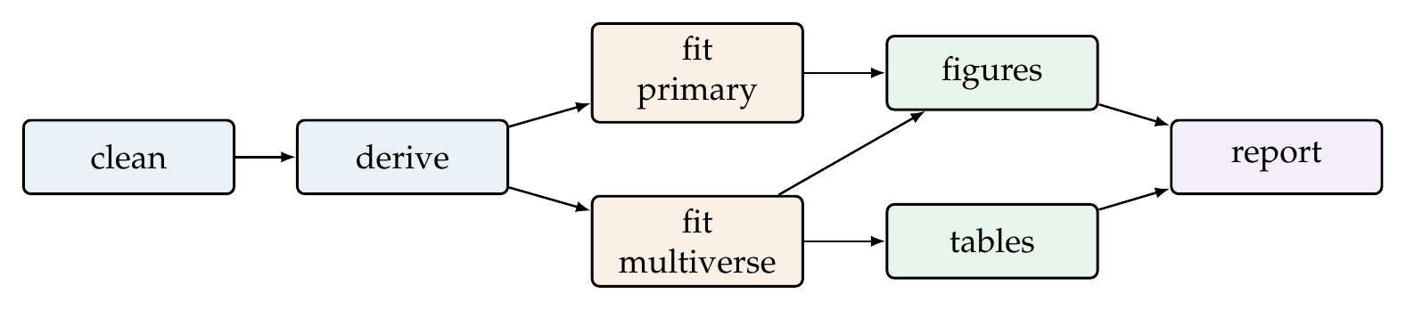
Note. Each node is a build target and each arrow a dependency. The primary and multiverse fits both depend on the derived data and are independent of each other, so a change to the multiverse code reruns only its branch. The graph is generated by the pipeline tool rather than drawn by hand, so it cannot drift from the actual analysis, which is its value as documentation.
Table 36.2. The Seeds-and-Stochastics Registry (Template)
| Stochastic step | Seed | Where set | Parallel-safe? |
|---|---|---|---|
| Data simulation | 20260820 | gen script | n/a (single) |
| Bootstrap CIs | 20260901 | analysis | yes (per-worker streams) |
| MCMC chains | 20260902 | fit script | yes (per-chain) |
| Multiple imputation | 20260903 | impute script | yes (per-imputation) |
Note. One row per stochastic step, recording the seed, where it is set, and whether parallel workers are seeded independently. The most common reproducibility failure in parallel computation is a single global seed with unseeded workers, which makes the run irreproducible despite appearing seeded.
In Practice • In Practice: when the pipeline fights you
Two failures recur. A pipeline that will not invalidate, rerunning nothing after a code change, usually means the change was to a file the pipeline does not track as a dependency, and the fix is to declare the dependency explicitly rather than to force a rebuild, which hides the problem. A locked environment that will not restore, failing to reinstall a pinned package, usually means a system-level library or a removed package version, and the pragmatic triage is to record the failure, install the nearest available version, and document the substitution rather than abandon the lock. The discipline is not to make reproducibility perfect on the first try but to make every deviation visible, so that a reader knows exactly where the rebuild departed from the original.
36.3 Reporting Standards, Harmonized
The reporting checklists that accumulated through the book, for mixed models, growth models, invariance, mixtures, dynamic models, networks, survival, and flexible and machine-learning methods, share a common spine, and Table 36.3 states it once with the per-family additions noted. The spine has seven elements: a description of the data structure, missingness, and compliance; a specification of the model as equations or unambiguous prose with the syntax in a supplement; a statement of the estimation method, software, versions, settings, and convergence diagnostics; the inference procedure with its degrees of freedom or diagnostics; the estimands and their effect sizes; the sensitivity results; and the visualization obligations. The per-family deltas are specific and are what a methods reviewer now checks: a growth model must report its time coding and its random-effect structure, a dynamic model its stationarity handling and its detrending, a mixture model its enumeration criteria and its class-size caveats, a survival model its proportional-hazards check, a flexible model its smoothing basis and its concurvity. Journal reality intrudes here, because word limits force material to supplements, and the discipline is to move detail to the supplement without hiding the result, so that a reader of the main text learns what was found and a reader of the supplement can rebuild it.
Table 36.3. The Harmonized Reporting Checklist (Spine and Family Deltas)
| Spine element | What to report (with family deltas) |
|---|---|
| Data structure | Persons, occasions, timing regularity, outcome type; missingness rate and mechanism; compliance |
| Specification | Model equations or unambiguous prose; syntax in supplement. Growth: time coding, random structure. Dynamic: stationarity, detrending. Mixture: enumeration criteria |
| Estimation | Method, software, versions, settings; convergence (Rhat/ESS; Heywood/singularity) |
| Inference | Test or interval method; degrees of freedom or diagnostics |
| Estimands | The target quantities and their effect sizes, not only \(p\) |
| Sensitivity | The mandatory forks run and their results; divergences named |
| Visualization | Data shown, not only models; uncertainty displayed |
Note. The spine is common to every model family; the deltas are the family-specific items a reviewer now expects. A report that covers the spine and its family delta is auditable; one that omits the estimation versions or the sensitivity results is not, however significant its headline.
36.4 The Sensitivity Doctrine, Formalized
Every methods chapter insisted on sensitivity analysis, and the insistence can now be formalized as a registry and a protocol. The fork registry, Figure 36.4 and Table 36.4, catalogues the analytic forks that recur by model family, the centering variants, the time codings, the random-structure alternatives, the missingness models, the detrending and lag choices, the enumeration and tuning decisions, and marks each as must-run or context-dependent. The protocol is the multiverse: preregister the fork set, run it systematically over the pipeline’s grid, and report the result as a specification-summary display that shows every estimate with the analytic choices behind it, so that the pattern of divergence becomes visible. The crucial interpretive move is that the forks which move the conclusion are the finding, because a conclusion robust to every defensible choice is strong precisely to the degree that the multiverse could have overturned it and did not, and a conclusion that flips on a centering decision is a conclusion about the centering. What separates a multiverse from p-hacking is disclosure and pre-specification: the multiverse reports all specifications, the p-hack reports the flattering one.
The exemplar makes this concrete. The question is a within-person one, whether a person’s negative affect rises on occasions when that person’s stress is higher than usual, estimated on the intensive-longitudinal affect_ema records, and the primary analysis, a within-person-centered random-slope multilevel model, estimates the reactivity at 0.35 with a standard error of 0.02. The micro-multiverse re-estimates it across a grid of twenty-four defensible specifications, crossing the centering, the random structure, the lag, and the covariate set, and Figure 36.5 shows the result: every one of the twenty-four specifications returns a positive reactivity, in a tight band from 0.31 to 0.36, so the conclusion that this reactivity is real and positive is robust to every fork, and the fork that moves the magnitude most is the covariate set, controlling for concurrent positive affect pulling the estimate down slightly. The honest paragraph writes itself from the display: the reactivity is positive across all defensible specifications, its magnitude is stable near a third of a scale point of negative affect per unit of within-person stress, and no analytic choice overturns the conclusion, which is the strongest thing a single study can say and is sayable only because the multiverse was run and reported rather than a single specification chosen.
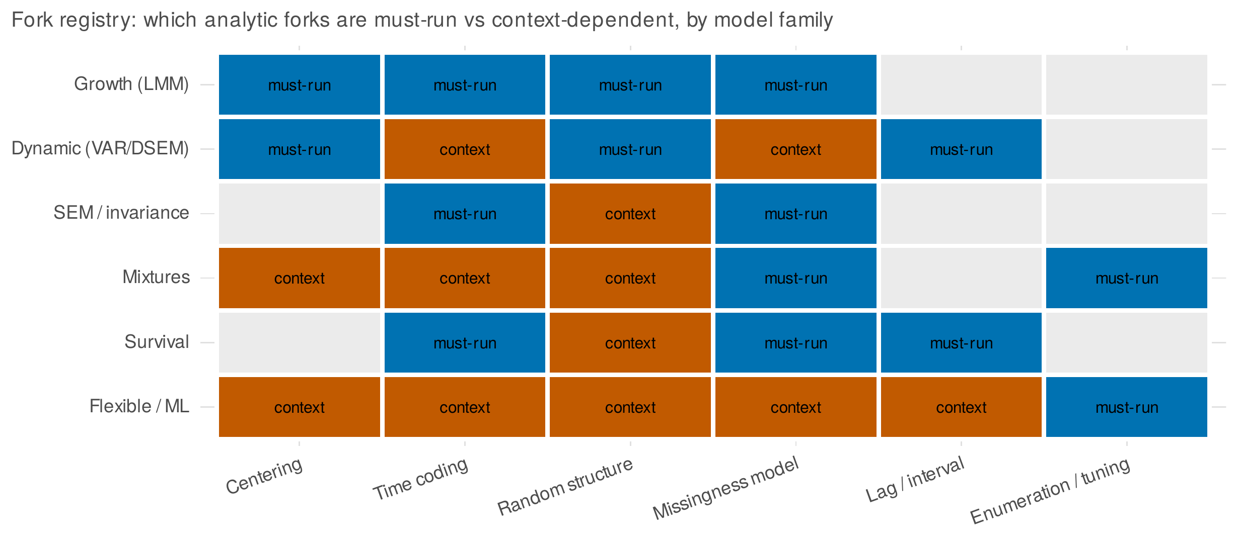
Note. Rows are model families, columns are recurring analytic forks, and cells mark a fork as must-run (blue), context-dependent (orange), or not applicable (grey) for that family. A growth model must run its centering, time coding, random structure, and missingness forks; a survival model must run its time coding, missingness, and interval forks. The registry turns the book’s scattered sensitivity advice into a checklist that a preregistration can commit to in advance.
Table 36.4. The Fork Registry (Selected Families)
| Family | Recurring forks | Must-run |
|---|---|---|
| Growth (LMM) | Centering; time coding; random structure; missingness | All four |
| Dynamic (VAR/DSEM) | Detrending; lag order; centering; stationarity | Detrending; lag |
| Mixture | Enumeration criterion; starts; covariate handling | Enumeration |
| Survival | Time coding; PH check; competing risks; missingness | Time coding; PH |
| Flexible / ML | Basis / tuning; cross-validation scheme; regularization | CV scheme; tuning |
Note. The must-run column names the forks whose variation is not optional to examine, because their default choices are known to move conclusions in that family. The context-dependent forks are run when the design or data make them live. Committing to this set in a preregistration is what makes a sensitivity portfolio confirmatory rather than exploratory.
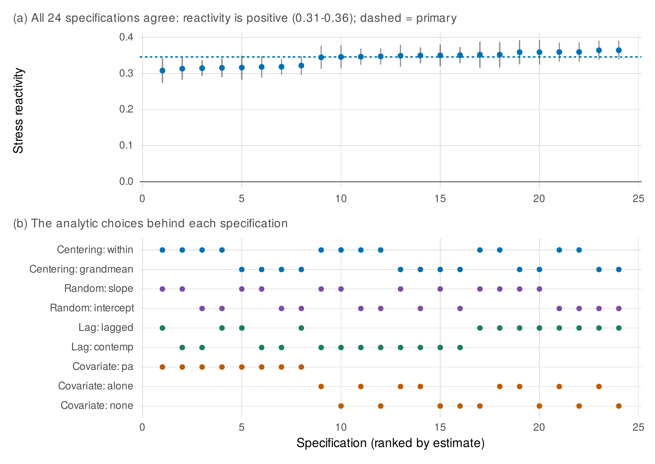
Note. Panel (a): the within-person stress reactivity estimated under each of twenty-four defensible specifications, sorted, with confidence intervals; all are positive and lie in a narrow band around the primary estimate (dashed). Panel (b): the analytic choices behind each specification, one row per fork level. The specifications with the smallest estimates are those that control for concurrent positive affect, identifying the covariate set as the fork that moves the magnitude; no fork changes the sign or the qualitative conclusion. That robustness, visible only because the whole grid was run, is the finding.
36.5 Preregistration for Longitudinal Research
Preregistration buys a specific thing, the separation of confirmatory from exploratory analysis, and it does not buy freedom from thought or a guarantee of truth. For longitudinal and experience-sampling research it has particular shapes, and Table 36.5 maps what can be bound in advance against what must remain data-contingent. A great deal is bindable even when model-building is genuinely iterative: the estimand, the primary specification, the mandatory fork set, the inclusion and compliance rules, and the decision tree that governs how the model will be built are all specifiable before the data are seen, and the honest middle path is to preregister the decision tree, the rule for how choices will be made, rather than a single fixed endpoint that real data will force you to abandon. Secondary and archival data, on which much longitudinal work rests, remain partly preregisterable: the variables not yet examined, the analyses to be run on a held-out split, and the sensitivity set can be committed even when the data already exist, because preregistration disciplines the analyst, not the data. Deviations are inevitable and are not failures; what matters is that they are logged and reported, so that a reader can see where the analysis departed from its plan and judge the departure. The experience-sampling preregistration templates that the field has developed, in the lineage of Kirtley and colleagues, walk through the sections a dense within-person design requires, and a filled template for the clinical exemplar of Chapter 33 would specify its sampling scheme, its compliance handling, its primary within-person estimand, and its sensitivity set before a single beep were analyzed.
Table 36.5. Preregistration Coverage Map for Longitudinal Research
| Decision | Bindable in advance? | Note |
|---|---|---|
| Estimand and primary model | Yes | The core commitment |
| Mandatory fork set | Yes | From the fork registry |
| Inclusion / compliance rules | Yes | Specify thresholds a priori |
| Model-building strategy | Yes, as a decision tree | Bind the rule, not the endpoint |
| Exact random structure | Often data-contingent | Bind the selection rule |
| Post hoc dynamics | No (exploratory) | Report as exploratory |
Note. The honest position is neither that everything must be fixed in advance, which iterative model-building makes impossible, nor that nothing can be, which abandons the confirmatory-exploratory distinction. Binding the decision tree, the rule by which choices will be made, preserves the distinction while allowing the data to inform the model.
Common Pitfall • Preregistration theater and buried sensitivity
Two failures hollow out these practices. Preregistration theater is the citation of a vague preregistration as though it were a strong one: a document that preregisters “we will run mixed models” binds nothing, because it does not name the estimand, the specification, or the decision rule, and a reader who sees a preregistration badge should read the document, not the badge. Buried sensitivity is the relegation of a sensitivity portfolio to a supplement with no synthesis in the main text, so that twenty-four specifications sit in a table no one reads while the abstract reports one: the sensitivity analysis earns its credibility only when its pattern is stated in the main text, as the honest paragraph of the exemplar states it. Both failures share a form, the appearance of rigor without its substance, and both are defeated by the same remedy, which is to say in the main text what was done and what it showed.
36.6 Writing and Archiving
Writing longitudinal results well begins with the estimand: a topic sentence that names the target quantity, “the within-person reactivity of negative affect to stress was positive and stable across specifications,” orients a reader as a sentence about significance does not. The drafting workflow is figures-first, building the display that shows the result before the prose that describes it, because a result that cannot be shown usually cannot be trusted, and the visualization obligations of the reporting checklist are met by drawing the data, not only the model. Uncertainty language is a discipline of its own, and Table 36.6 pairs the phrases to avoid with their honest replacements, because the difference between “stress causes negative affect” and “on higher-stress occasions, negative affect was higher within person” is the difference between a claim the design cannot support and one it can. Structuring a multi-model results section means marking its lanes, a primary lane, a sensitivity lane, and an exploratory lane, with headers that enforce the epistemics so that a reader never mistakes an exploratory dynamics analysis for a confirmatory one.
Table 36.6. Uncertainty Language: Phrases to Avoid and Their Replacements
| Avoid | Prefer |
|---|---|
| “X causes Y” (from observational within-person data) | “On occasions when X was higher, Y was higher within person” |
| “The effect was significant” | “The estimate was 0.35, 95% CI [0.31, 0.38]” |
| “The groups did not differ” | “The difference was 0.02, 95% CI [\(-0.10\), 0.14], inconclusive” |
| “The partner effect shows influence” | “The partner’s predictor forecast the outcome; influence is not established” |
| “Variability precedes decline” (as a law) | “Variability rose before the mean in these data, a modest person-level association” |
Note. The replacements are longer because they are more exact: they state the estimand, attach the uncertainty, and refuse the causal or general claim the design does not support. The habit of the replacements is the habit of honest longitudinal writing.
Archiving closes the loop the first chapter opened. A public repository for a longitudinal study has an anatomy, Figure 36.6, of raw and derived data, code, a codebook, the preregistration, and the manuscript, tiered so that what can be open is open and what must be protected is access-controlled. The protection matters most for intensive longitudinal data, whose dense behavioral traces are re-identifiable in ways that sparse survey data are not: a sequence of timestamps and locations can single out a person even when names are removed, and Table 36.7 lists the techniques, timestamp coarsening, geodata removal, and the k-anonymity intuition that no record should be unique on its quasi-identifiers, with what each protects against and what it costs. When the raw traces cannot be safely opened, a synthetic companion generated from the fitted model, the very device this book has used for every worked example, lets a reader rebuild the analysis without exposing a participant, which is a fitting closing symmetry: the simulated datasets that taught the methods are also the template for sharing real ones safely.
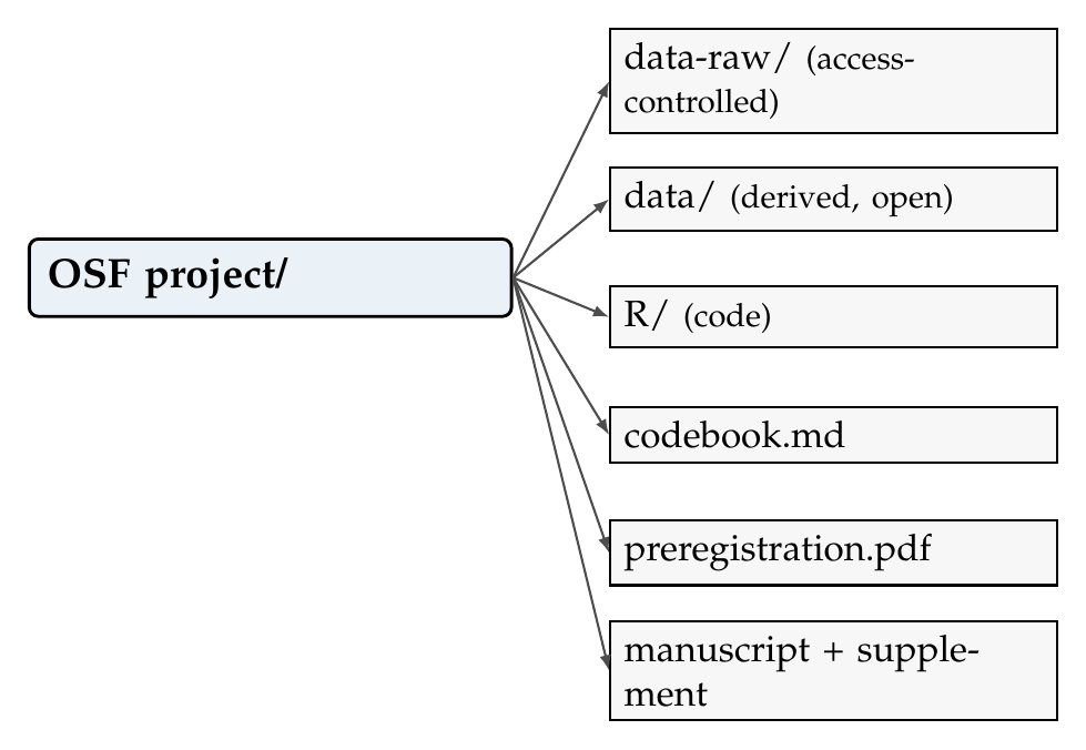
Note. A tiered repository: derived data, code, codebook, preregistration, and manuscript are open, while raw intensive data, which can re-identify participants, are access-controlled. When even a tiered release is unsafe, a synthetic dataset generated from the fitted model lets a reader rebuild the analysis without exposing anyone, the same device this book used to teach every method.
Table 36.7. De-Identification Techniques for Intensive Longitudinal Data
| Technique | Protects against | Cost |
|---|---|---|
| Timestamp coarsening | Re-identification by exact timing | Loses fine within-day dynamics |
| Geodata removal | Location-based identification | Loses spatial covariates |
| \(k\)-anonymity on quasi-identifiers | Uniqueness on demographics | May require aggregation |
| Synthetic companion data | All direct re-identification | Preserves modeled, not raw, structure |
Note. Each technique trades protection against analytic fidelity. Dense behavioral traces are re-identifiable in ways sparse data are not, so the default for intensive longitudinal data is a tiered release with the raw traces access-controlled, and a synthetic companion when open rebuilding matters more than raw fidelity.
In Practice • Ethics: open data and the re-identification duty
The push to open data is right, and it collides with a duty that intensive longitudinal research makes acute: the denser the behavioral record, the easier a de-identified participant is to re-identify, so that a fully open release of raw experience-sampling traces can breach a confidence that consent did not knowingly waive. The resolution is not to abandon openness but to tier it, opening the derived data and code that let others rebuild the analysis while access-controlling the raw traces that could expose a person, and to obtain consent that describes the sharing plan honestly rather than promising an openness that endangers the participant. The duty of care and the duty of openness are both real, and the tiered repository with a synthetic companion is how a study honors both.
Software Note • Software Note
The reproducibility stack is fast-moving, and specific tools should be checked against their current documentation before adoption. At the time of writing, the common longitudinal stack is a package-locking tool that records and restores pinned versions, a pipeline tool that declares build targets and their dependencies and reruns only what changed, a literate-analysis system that interleaves prose and code so the narration cannot drift from the computation, and a repository client that deposits the project to a public archive. The exact application programming interfaces of these tools change across versions; what does not change is the discipline they encode, immutable inputs, pinned versions, declared dependencies, registered seeds, and archived outputs, which can be practiced with any tooling or none. A minimum viable adoption, for a reader whose collaborators do not yet work this way, is seeds and versioned filenames first, then a locked environment, then the checklists, then a managed pipeline, then the full sensitivity portfolio.
36.7 The End-to-End Exemplar
The exemplar can now be read as a whole, a compact study executed through the entire system. The question, phrased to fix its estimand, is whether negative affect rises within a person on higher-stress occasions, which the estimand-phrasing guide routes to a within-person multilevel model. The preregistration, filed before analysis, names that estimand, the within-person-centered random-slope specification as primary, the twenty-four-cell fork grid as the mandatory sensitivity set, and a decision rule for the random structure. The pipeline builds the derived data from the immutable raw beeps, fits the primary model and the multiverse as independent branches, and draws the displays, every stochastic step seeded from the registry. The primary analysis returns a reactivity of 0.35, and Figure 36.7 shows the result the way it should be shown, not as a single number but as a distribution of person-specific reactivities around the pooled estimate, positive on average and varying across persons, so that the between-person heterogeneity in a within-person effect is visible rather than hidden. The sensitivity portfolio, the specification curve of Figure 36.5, confirms the estimate is positive across all twenty-four specifications and identifies the covariate set as the only fork that moves it appreciably. The reporting audit against the harmonized checklist confirms the data structure, specification, estimation versions, inference, estimand, sensitivity, and visualization are all present. And the archive deposits the derived data, the code, the codebook, the preregistration, and a synthetic companion to a tiered repository. Each move traces to its chapter, and the whole is a study a stranger could rebuild.
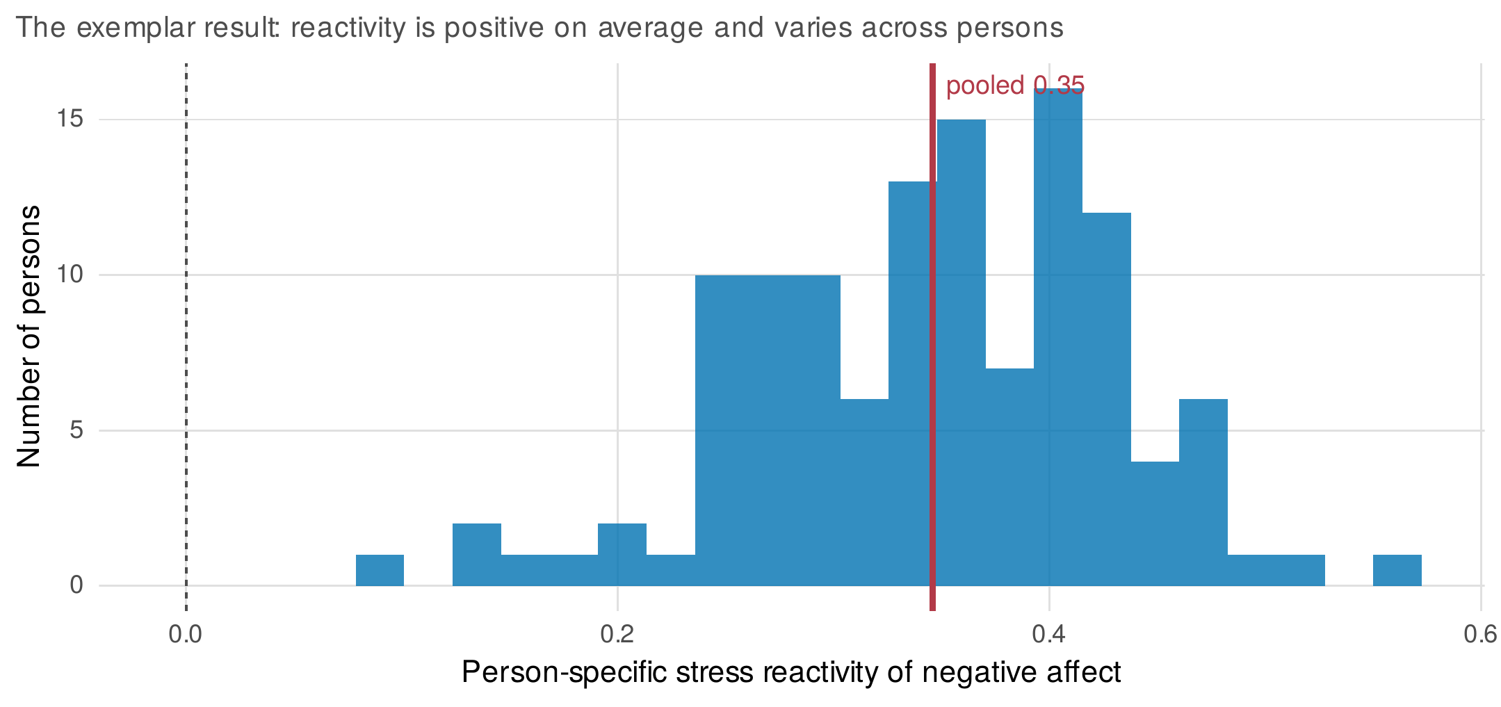
Note. The person-specific stress reactivities of negative affect, with the pooled estimate marked. The effect is positive for nearly every person and varies in magnitude across persons, the between-person heterogeneity in a within-person effect that a single pooled number would conceal. Showing the distribution rather than the point is the visualization obligation the reporting checklist imposes and the estimand-first writing the last section urged.
The book set out to make change analyzable, and it end where it began, at the map. Chapter 1 drew that map as a promise to a reader who did not yet know which method to use; this chapter has walked it as an audit, with every method built, every checklist harmonized, every doctrine formalized, and the whole shown working on one honest example. The claim the two bookend chapters make together is that analyzing change is not a catalogue of techniques to be memorized but a discipline to be practiced: name the estimand, choose the method the question implies, run the sensitivities its assumptions demand, report what was done so that a stranger can see it, and archive it so that a stranger can rebuild it. The reader who has come this far can do this, and that was the point.
Chapter Summary
This capstone consolidated the book into a workflow. The master decision system crosses the question family with the data structure and the defensible assumptions to yield a primary analysis, a mandatory sensitivity set, and a claim ceiling, and Figure 36.1 completes the map Figure 1.5 began. The reproducible-project section fixed the disciplines of immutable raw data, locked environments, managed pipelines, and a seed registry. The harmonized checklist stated the reporting spine common to every model family with its per-family deltas. The sensitivity doctrine was formalized as a fork registry and a multiverse protocol, and the exemplar’s specification curve showed a within-person reactivity positive across all twenty-four defensible specifications, robust to every fork but the covariate set, which is the strongest claim a single study can make and is sayable only because the whole grid was run and reported. Preregistration was treated at working depth, binding the decision tree rather than a fixed endpoint and remaining partly available even for archival data. Writing was made estimand-first with disciplined uncertainty language, and archiving was made tiered, with a synthetic companion protecting the re-identifiable traces of intensive data. The book ends where it began, at the map, now walked rather than promised: name the estimand, choose the method, run the sensitivities, report honestly, archive openly. The reader can do this.
Appelbaum, M., Cooper, H., Kline, R. B., Mayo-Wilson, E., Nezu, A. M., & Rao, S. M. (2018). Journal article reporting standards for quantitative research in psychology: The APA Publications and Communications Board task force report. American Psychologist, 73(1), 3–25. https://doi.org/10.1037/amp0000191
Chambers, C. D. (2013). Registered Reports: A new publishing initiative at Cortex. Cortex, 49(3), 609–610. https://doi.org/10.1016/j.cortex.2012.12.016
Gelman, A., & Loken, E. (2014). The statistical crisis in science. American Scientist, 102(6), 460–465. https://doi.org/10.1511/2014.111.460
Kirtley, O. J., Lafit, G., Achterhof, R., Hiekkaranta, A. P., & Myin-Germeys, I. (2021). Making the black box transparent: A template and tutorial for registration of studies using experience-sampling methods (ESM). Advances in Methods and Practices in Psychological Science, 4(1), Article 2515245920924686. https://doi.org/10.1177/2515245920924686
Klein, O., Hardwicke, T. E., Aust, F., Breuer, J., Danielsson, H., Hofelich Mohr, A., IJzerman, H., Nilsonne, G., Vanpaemel, W., & Frank, M. C. (2018). A practical guide for transparency in psychological science. Collabra: Psychology, 4(1), Article 20. https://doi.org/10.1525/collabra.158
Landau, W. M. (2021). The targets R package: A dynamic Make-like function-oriented pipeline toolkit for reproducibility and high-performance computing. Journal of Open Source Software, 6(57), Article 2959. https://doi.org/10.21105/joss.02959
Meyer, M. N. (2018). Practical tips for ethical data sharing. Advances in Methods and Practices in Psychological Science, 1(1), 131–144. https://doi.org/10.1177/2515245917747656
Munafo, M. R., Nosek, B. A., Bishop, D. V. M., Button, K. S., Chambers, C. D., Percie du Sert, N., Simonsohn, U., Wagenmakers, E.-J., Ware, J. J., & Ioannidis, J. P. A. (2017). A manifesto for reproducible science. Nature Human Behaviour, 1(1), Article 0021. https://doi.org/10.1038/s41562-016-0021
Nosek, B. A., Ebersole, C. R., DeHaven, A. C., & Mellor, D. T. (2018). The preregistration revolution. Proceedings of the National Academy of Sciences, 115(11), 2600–2606. https://doi.org/10.1073/pnas.1708274114
Peikert, A., & Brandmaier, A. M. (2021). A reproducible data analysis workflow with R Markdown, Git, Make, and Docker. Quantitative and Computational Methods in Behavioral Sciences, 1, Article e3763. https://doi.org/10.5964/qcmb.3763
Simmons, J. P., Nelson, L. D., & Simonsohn, U. (2011). False-positive psychology: Undisclosed flexibility in data collection and analysis allows presenting anything as significant. Psychological Science, 22(11), 1359–1366. https://doi.org/10.1177/0956797611417632
Simonsohn, U., Simmons, J. P., & Nelson, L. D. (2020). Specification curve analysis. Nature Human Behaviour, 4(11), 1208–1214. https://doi.org/10.1038/s41562-020-0912-z
Steegen, S., Tuerlinckx, F., Gelman, A., & Vanpaemel, W. (2016). Increasing transparency through a multiverse analysis. Perspectives on Psychological Science, 11(5), 702–712. https://doi.org/10.1177/1745691616658637
Trull, T. J., & Ebner-Priemer, U. W. (2020). Ambulatory assessment in psychopathology research: A review of recommended reporting guidelines and current practices. Journal of Abnormal Psychology, 129(1), 56–63. https://doi.org/10.1037/abn0000473
Van Lissa, C. J., Brandmaier, A. M., Brinkman, L., Lamprecht, A.-L., Peikert, A., Struiksma, M. E., & Vreede, B. M. I. (2021). WORCS: A workflow for open reproducible code in science. Data Science, 4(1), 29–49. https://doi.org/10.3233/DS-210031
Wicherts, J. M., Veldkamp, C. L. S., Augusteijn, H. E. M., Bakker, M., van Aert, R. C. M., & van Assen, M. A. L. M. (2016). Degrees of freedom in planning, running, analyzing, and reporting psychological studies: A checklist to avoid p-hacking. Frontiers in Psychology, 7, Article 1832. https://doi.org/10.3389/fpsyg.2016.01832
Wilson, G., Bryan, J., Cranston, K., Kitzes, J., Nederbragt, L., & Teal, T. K. (2017). Good enough practices in scientific computing. PLOS Computational Biology, 13(6), Article e1005510. https://doi.org/10.1371/journal.pcbi.1005510