Chapter 35
Applications in Social, Personality, Organizational, and Health Psychology
These are the domains where diary and experience-sampling methods were invented, and where the book’s within-person thread pays its widest dividends, because here the phenomena of interest are processes that live inside days and between people rather than differences that sit between persons. This chapter, the third and last of the applications part, works three questions that the field has often mishandled for want of the right within-person tools. The first reframes personality itself: a trait is not a single number but a distribution of states, and the person’s mean, the person’s variability, and the person’s contingent reactivity are all personality parameters, estimated from intensive data and carried into the nomological network without the uncertainty laundering that plagues two-stage analyses. The second, the chapter’s investment, is the dyadic daily process, where two interdependent streams must be modeled together, and where the specification most researchers reach for is subtly wrong in ways that contaminate the very effects they report; the actor-partner interdependence model in its multilevel form, built with the centering discipline the double decomposition demands, is developed here at a depth the scattered literature rarely reaches. The third turns to the rhythms of work and recovery, where the weekly cycle is not a nuisance to be controlled but the theory to be tested, and where the evening’s psychological detachment forecasts the next morning’s vigor. The three cases share a commitment and a caution: the commitment is that within-person structure is where the action is, and the caution is that a partner effect is not automatically an influence, a variability index is not automatically a trait, and a weekday coefficient is not automatically a control. Each case is written as an empirical paper would be, with the reasoning a finished paper conceals made visible.
Learning Objectives
After working through this chapter, you should be able to: (1) treat personality as density distributions of states, estimating the mean, the within-person variability, and the contingent reactivity as trait parameters, and carrying them into trait-outcome analyses with their uncertainty propagated; (2) model dyadic daily data with a multilevel actor-partner interdependence model, distinguishing within-person from between-couple effects and actor from partner effects, and using the centering that keeps them separate; (3) estimate dyadic growth and cross-partner lead-lag structure, and interpret partner effects with the caution their confounds require; (4) test cyclical organizational phenomena as theory rather than decoration, and estimate within-person recovery across the night boundary; (5) handle the design realities of these domains, from event-contingent recording to partner privacy to organizational consent hierarchies; and (6) translate within-person findings for audiences trained on between-person constructs without overclaiming.
35.1 The Terrain: Processes Where People Live
The questions of social, personality, and organizational psychology that this book can serve are questions about within-person process, and they fall into a few families that route to the tools developed earlier. The expression of a state and its contingencies, how much a person’s momentary extraversion or affect varies and what situations move it, is a distribution question answered by the variability and location-scale tools of Chapters 7 and 16. The transmission of states between people, whether one partner’s support lifts the other’s intimacy and who leads whom day to day, is a dyadic question answered by the multilevel models of Chapter 23 extended to two interdependent members and by the coupling methods of Chapter 25. The rhythms of work and recovery, the weekly cycle and the restoration of a weekend, are cyclical questions answered by the trigonometric and cyclic-smooth tools of Chapters 23 and 30. And the couplings of behavior and health across the day are dynamic questions answered by the same within-person machinery. Figure 35.1 draws the routing and Table 35.1 lists the families with estimands and exemplar literatures.
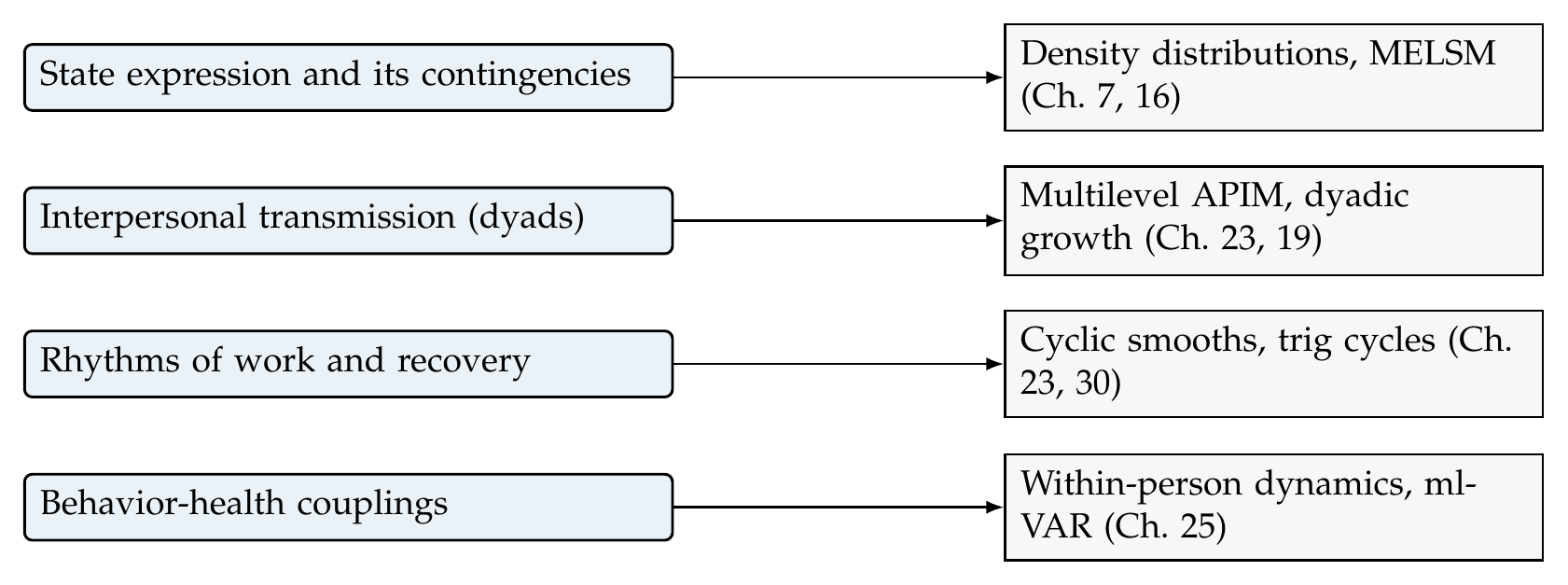
Note. Each family of within-person question routes to the tools that answer it. The design lineage runs from the Rochester Interaction Record and the event-contingent tradition of Wheeler and Reis through modern smartphone experience sampling, but the analytic families are stable, and naming the family remains the first analytic act.
Table 35.1. Question Taxonomy, Estimands, Chapters, and Exemplars
| Question family | Estimand | Chapters | Exemplar |
|---|---|---|---|
| State distributions | Person mean, SD, reactivity | 7, 16 | Fleeson (2001) |
| Dyadic transmission | Actor/partner within effects | 23, 25 | Laurenceau et al. (1998) |
| Work rhythms | Cycle shape; recovery lag | 23, 30 | Sonnentag (2003) |
| Behavior-health | Within-person coupling | 25 | Butler (2011) |
Note. The estimand is the discipline. These domains share a chronic communication problem, that their audiences are trained on between-person constructs, and the last section returns to it.
35.2 Case Study A: Personality as Distributions of States
The reconciliation of states and traits that Fleeson (2001) proposed dissolves an old dispute by a change of object: a personality trait is not a person’s single characteristic value but the density distribution of that person’s momentary states, and the parameters of that distribution, the mean, the spread, and the way the state depends on the situation, are the trait. This reframing turns intensive longitudinal data into a personality-measurement instrument, and it is the content of Case A, worked on the affect_ema records reframed as a personality study: 120 persons, sampled roughly six times a day for two weeks, whose momentary positive affect, negative affect, and stress are the states from which distribution parameters are estimated.
35.2.1 Distribution Parameters as Personality
Figure 35.2 shows the raw object of study, the distribution of momentary positive affect for a spread of persons, and it makes the essential point visually: persons differ not only in where their distribution sits but in how wide it is, so that two people with the same average affect can differ sharply in their variability, and both facts are personality. Estimating the parameters properly means resisting the temptation to compute a raw within-person standard deviation and treat it as a trait, because such an index confounds true variability with measurement error and with the person’s mean, the confound Baird, Le, and Lucas (2006) documented; the location-scale model of Chapter 16 is the repair, modeling the person’s mean and the logarithm of the person’s residual variability jointly with the person’s contingent reactivity as a random slope. Fit to these data, the three parameters are all substantial and person-varying: the person means of negative affect average 2.02 with a between-person standard deviation of 0.44, the within-person variabilities average 0.56 with a between-person standard deviation of 0.10, and the stress reactivity, the degree to which a person’s negative affect rises with momentary stress, averages 0.35 with a between-person standard deviation of 0.08. Table 35.2 sets out which distribution parameter operationalizes which personality construct.
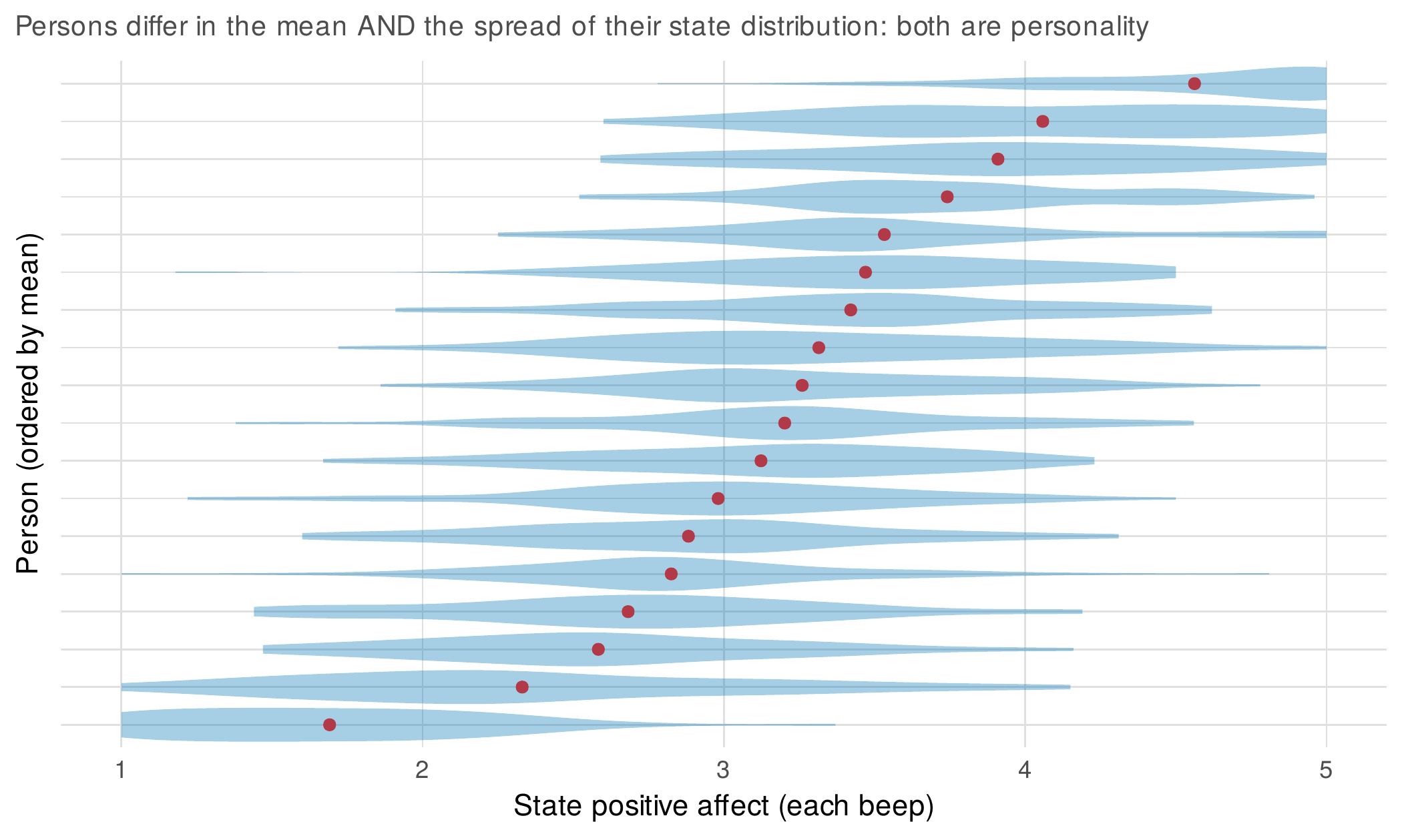
Note. Each row is one person’s distribution of momentary positive affect across two weeks of sampling, ordered by the person mean (red points). Persons differ in the location of the distribution and, independently, in its spread; both are stable personality parameters in the density-distribution view. A raw standard deviation read off these distributions would confound true spread with measurement error and with the mean, which the location-scale model of Chapter 16 corrects.
35.2.2 Stability and the Anti-Plug-In Discipline
For a distribution parameter to count as a trait it must be stable, and splitting the study into its two weeks and correlating each parameter across the halves gives the empirical verdict: the person mean is highly stable, correlating 0.90 across the halves, the within-person variability is moderately stable at 0.56, and the reactivity is the noisiest at 0.37, which is the pattern the density-distribution literature has converged on, mean level robustly trait-like and the higher-order parameters real but harder to pin down in two weeks of data. The stability numbers matter for the next step, which is carrying these parameters into trait-outcome analyses, because a parameter estimated with error is a predictor measured with error, and treating it as if it were known is the plug-in fallacy that Chapter 16 warned against. Figure 35.3 shows the consequence in a controlled demonstration: when a person-level outcome truly depends on the person’s variability, regressing the outcome on the plug-in estimate of variability attenuates the effect, here from a true 0.50 to a naive 0.45, and understates its uncertainty, because the noise in the estimated variability is ignored; propagating that estimation uncertainty, through an errors-in-variables correction that uses the known sampling variance of a standard deviation, restores the effect to 0.55 and widens the interval honestly. The discipline is simple to state and often ignored: a distribution parameter entering a between-person model carries its own uncertainty, and that uncertainty belongs in the second-stage inference.
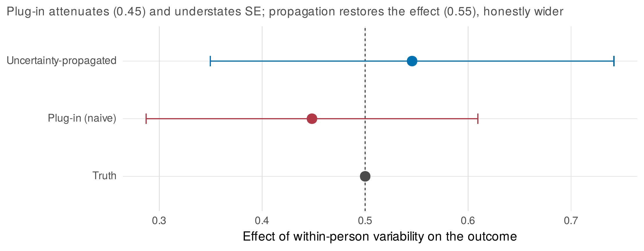
Note. A person-level outcome depends on the person’s true within-person variability, estimated here from about twenty-five usable occasions. The plug-in analysis regresses the outcome on the point estimate, attenuating the effect and reporting too narrow an interval. Propagating the estimation uncertainty, via an errors-in-variables correction using the known sampling variance of a standard deviation, restores the effect and widens the interval to its honest width. The attenuation grows as the parameter rests on fewer occasions.
Common Pitfall • The raw variability index as a trait
The single most common error in this literature is to compute a person’s raw within-person standard deviation, or a mean successive difference, and enter it into a between-person analysis as though it were a clean trait. Three problems compound. The index confounds true variability with measurement error, so that unreliable measures manufacture spurious variability. It is entangled with the mean, because bounded scales compress variability near the ceiling and floor, so that a person’s variability and level cannot be read independently from the raw index. And it is estimated with sampling error that the second-stage analysis then ignores, attenuating and over-precisely reporting any effect. The location-scale model of Chapter 16 addresses the first two by modeling the mean and the log-variability jointly, and the uncertainty propagation of Figure 35.3 addresses the third. A variability finding built on the raw index alone is not yet a finding about the person.
35.3 Case Study B: Dyadic Daily Process
Two people in a relationship generate two interdependent streams of daily data, and the central methodological fact is that the streams cannot be analyzed apart, because each partner’s outcome depends on both partners’ predictors and because the two members of a couple are more alike than two random individuals. Case B develops the analysis on the couples_diary records, a distinguishable-dyad study of 130 couples reporting daily support and intimacy across three weeks, with a known actor-partner structure, a satisfaction moderator, a between-couple confound, a common-fate growth process, and an asymmetric cross-partner lag, so that every claim can be checked against the truth. Figure 35.4 shows the data’s anatomy, the two aligned streams with their shared couple-days, and the section builds the model that respects it.
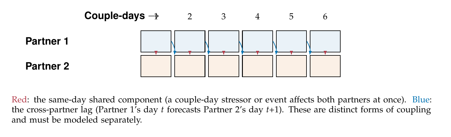
Note. Two partners generate aligned daily streams sharing the same couple-days. Coupling takes two distinct forms: a same-day shared component, in which an event moves both partners at once, and a lagged cross-partner component, in which one partner’s state forecasts the other’s on the following day. Conflating them, or ignoring the nonindependence entirely, misstates the interdependence that is the object of study.
35.3.1 Nonindependence and the Actor-Partner Model
The nonindependence is real and quantifiable: the dyadic intraclass correlation of intimacy, the share of variance lying between couples, is 0.34, far from the zero that an analysis of individuals would assume, and it is the reason a couple-level random effect is mandatory. The model that respects the dyadic structure is the actor-partner interdependence model in its multilevel form, in which each partner’s daily intimacy is regressed on the partner’s own support, the actor effect, and on the other partner’s support, the partner effect, with the two members’ days sharing a couple random intercept. Figure 35.5 draws the specification. The subtlety that the scattered applied literature routinely gets wrong is the centering: an actor effect is a within-person effect, the degree to which a partner’s intimacy rises on days when that partner’s support is higher than usual, and it is estimated cleanly only when support is centered within person, separating the day-to-day within-person association from the between-person association of people who give more support on average. Table 35.3 is the decision table that resolves the specification, crossing distinguishability, error structure, and centering.
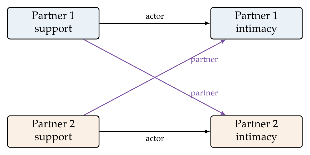
Note. Each partner’s intimacy depends on the partner’s own support (the actor effect) and on the other partner’s support (the partner effect, purple). Estimated in a multilevel model with support centered within person and a couple-level random intercept, the actor and partner effects are within-person daily effects, separated from the between-couple association. The paths shown are the within-person layer; the between-couple layer is a parallel set of couple-mean effects.
Table 35.3. Dyadic Specification Decision Table
| Decision | Options | Guidance |
|---|---|---|
| Distinguishability | Distinguishable (e.g. by role) vs. indistinguishable | Distinguishable: include member; indistinguishable: pairwise/double-entry with member-invariant effects |
| Error structure | One vs. two residual variances; within-day correlation | Allow a within-couple-day residual correlation; distinguishable dyads may need two residual variances |
| Centering | Within-person, grand-mean, or couple-mean | Within-person for the actor effect; couple-mean carries the between effect |
Note. The combination that most applied papers get wrong is grand-mean centering with a single residual variance, which contaminates the actor effect with the between-person association. The within-person centering in the last row is the resolver.
Fitting the properly centered model recovers the planted structure: the actor effect is 0.45 against a truth of 0.40, the partner effect is 0.19 against a truth of 0.20, and the between-couple effect of average support on intimacy is 0.59 against a truth of 0.60, so that the between-person association is genuinely larger than the within, exactly the double dissociation the centering is designed to reveal. Figure 35.6 shows these estimates against their truths and, crucially, shows the cost of the common error: an analyst who centers support only at the grand mean estimates the actor effect as 0.51, contaminated upward by the larger between-person association, an error of the same size as many published effects. Relationship satisfaction moderates the actor effect as planted, the within-person support-intimacy coupling being stronger in more satisfied couples, with a recovered interaction of 0.13 against a truth of 0.15. Table 35.4 is the glossary that keeps the four effects straight.
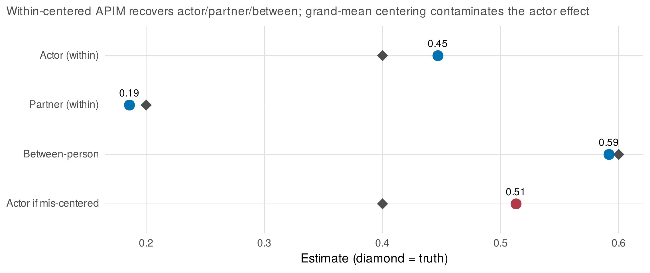
Note. The within-centered model recovers the actor (0.45), partner (0.19), and between-person (0.59) effects near their planted truths (diamonds). The bottom row shows the actor effect when support is centered only at the grand mean: it is pulled to 0.51, contaminated by the larger between-person association, an error that inflates the reported within-person coupling. Centering is not a technicality here; it is the difference between the effect you want and an effect you did not.
Table 35.4. The APIM Effect Glossary
| Effect | Meaning | Estimate (truth) |
|---|---|---|
| Actor, within | Own support on own intimacy, day to day | 0.45 (0.40) |
| Partner, within | Partner’s support on own intimacy, day to day | 0.19 (0.20) |
| Between-person | Average support on average intimacy | 0.59 (0.60) |
| Actor, mis-centered | The contaminated actor effect | 0.51 (should be 0.40) |
Note. The four quantities answer different questions. The within-person actor and partner effects are the daily interdependence; the between-person effect is a person-difference association; the mis-centered actor effect is neither, being a blend that no theory intends.
35.3.2 Dyadic Growth and Who Leads Whom
Beyond the daily couplings, the couple’s intimacy has a trajectory, and the dyadic growth model asks whether the two partners’ trajectories move together. Fitting a growth model with a couple-level random slope recovers a shared upward drift of 0.015 units per day, and the couple-level slope captures the common fate, the tendency of partners to rise and fall together over the study rather than independently, which Figure 35.7 displays for a sample of couples whose two trajectories track one another. The common-fate representation, in which a single couple-level trajectory drives both partners, is the theoretically apt alternative to a parallel-process model with two separate but correlated slopes when the causal story is one of shared circumstance rather than mutual influence, and choosing between them is a choice about what the couple is, not a fit contest. The final layer is the dynamic one, the question of who leads whom, and estimating the cross-partner lag on the intimacy residual recovers the planted asymmetry: Partner 1’s intimacy on one day forecasts Partner 2’s the next with a coefficient of 0.18, while the reverse path is only 0.07, so Partner 1 leads and Partner 2 follows, the lead-lag structure Figure 35.8 displays. The caution here is the one Chapter 25 pressed: a cross-partner lag is a temporal-predictive fact, not a demonstration of influence, because a shared unmeasured driver, a common daily stressor, or a third variable can manufacture the asymmetry, and the recurrence-based coordination methods of Chapter 32 offer a complementary view without resolving the causal question.
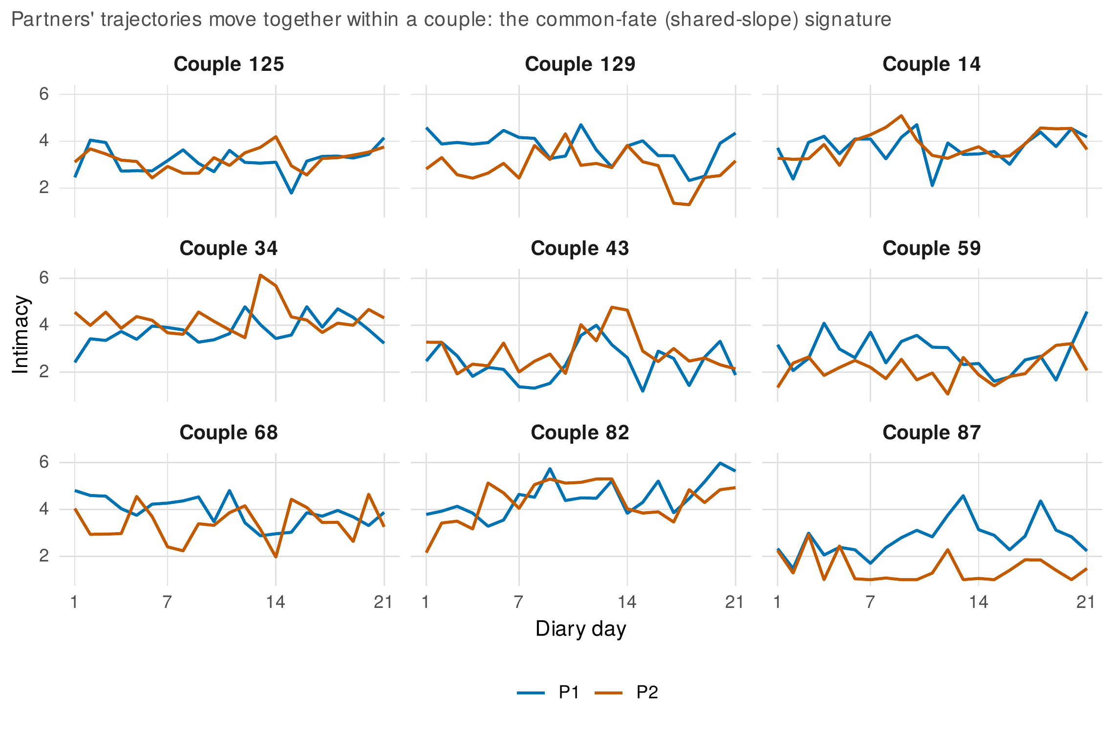
Note. Intimacy trajectories for nine couples, each partner a separate line. Within a couple the two partners’ trajectories move together, the common-fate signature that a couple-level random slope captures. When partners rise and fall together because they share circumstances, the common-fate model is the apt representation; when the story is mutual influence, a parallel-process model with cross-partner slope couplings is the alternative.
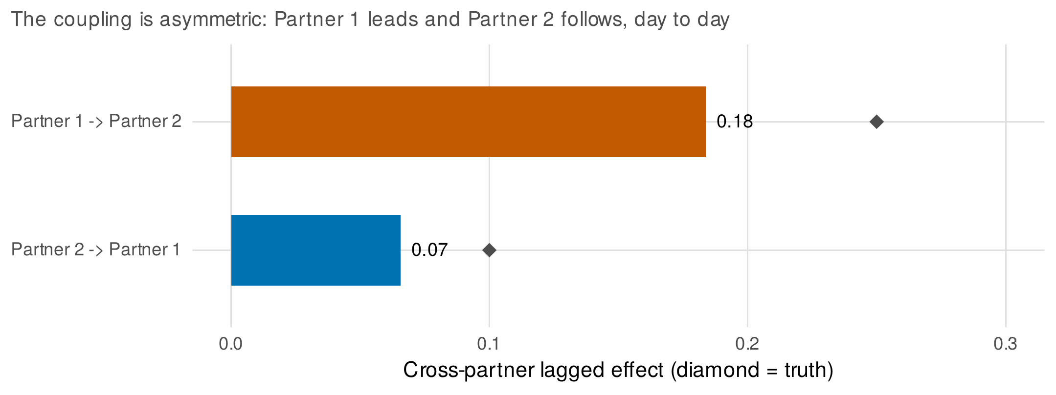
Note. The cross-partner lagged effects on the intimacy residual, controlling each partner’s own inertia. The coupling is asymmetric, Partner 1 leading (0.18) and Partner 2 following (0.07), recovering the planted asymmetry (diamonds). The lead-lag is a predictive fact, not a proof of influence: a shared daily driver can produce the same asymmetry, which is why the caution ledger of Chapter 25 applies.
In Practice • In Practice: running a couples diary
Dyadic diary studies add logistical burdens that single-person studies do not face. Recruitment must secure two committed participants per unit, and differential compliance, one partner completing more entries than the other, creates missing-data patterns that are not ignorable if compliance tracks the very processes under study. Privacy between partners is a design constraint, not an afterthought: entries must be collected so that one partner cannot read the other’s responses, which shapes the delivery platform and the consent. And the shared events that make dyadic data interesting, the arguments and reconciliations that both partners report, must be reconcilable across the two streams, which requires a common timestamping discipline. These are the realities behind the clean data matrix, and a methods section that ignores them invites the reviewer’s doubt.
In Practice • Ethics: interdependence and disclosure
Dyadic data carry a disclosure risk that individual data do not: one partner’s responses can reveal the other’s circumstances, and a release that de-identifies each individual may still expose a couple. Reporting an aggregate that rests on a small or distinctive subsample of couples can make a particular relationship recognizable to its members, and returning individual-level results to one partner can breach the other’s confidence. The duty of care extends to both members and to the dyad as a unit, which means consent that both partners understand, analysis outputs that cannot be traced to an identifiable couple, and a data-sharing plan that treats the couple, not only the person, as the unit to be protected.
Software Note • Software Note
The dyadic models here are fit with lme4, using a couple-level random intercept and support centered within person; a within-couple-day residual correlation, when needed for distinguishable dyads, is available through nlme’s correlation structures. The actor-partner model in a structural-equation framework, which allows correlated residuals and latent variables, is developed by Gistelinck and Loeys (2019); a Bayesian implementation through brms accommodates the two-member error structure and propagates uncertainty naturally, at the cost of longer computation. The density-distribution parameters of Case A are estimated with a location-scale model, available in brms and approximated here in stages, and the cross-partner lead-lag uses the residual vector-autoregression of Chapter 25. All scripts, seeded, accompany the chapter.
35.4 Case Study C: Workweek Rhythms and Recovery
The organizational literature on stress and recovery treats the week as a structure with meaning: strain accumulates across workdays, recovery happens in the evenings and on weekends, and the rhythm itself is the phenomenon, not a nuisance to be partialled out. Case C works these ideas on the work_week records, a two-week diary of 200 workers with a workday, evening, and morning architecture, a planted weekly cycle in vigor, a discontinuous weekend restoration, a within-person recovery effect linking the evening’s detachment to the next morning’s vigor, and a job-demands moderator, so that the theory-testing can be audited against a known process.
35.4.1 The Weekly Cycle as Theory
The weekly cycle is estimated two ways, and the contrast is instructive. A single trigonometric harmonic, a sine and cosine at the seven-day period, imposes a smooth sinusoid and recovers the planted cycle with a correlation of 0.95 to the truth; a cyclic spline, which lets the data choose the shape while enforcing that Sunday joins back to Monday, recovers it with a correlation of 0.91, theory-agnostic and nearly as efficient. Figure 35.9 shows both against the truth, a mid-week trough in vigor and a weekend peak, and Table 35.5 is the decision guide. The methodological point is that the choice between them is theoretical, not merely statistical: if theory predicts a smooth single-peaked rhythm, the trigonometric model encodes that prediction and tests it efficiently; if the shape is unknown or possibly multi-peaked, the cyclic smooth is the honest default; and treating the day of week as a set of free dummy variables, the third option, discards the cyclical structure entirely and is appropriate only when no rhythm is expected. A weekly cycle fit as decoration, a smooth added because the software offers one, is not the same as a weekly cycle fit as theory.
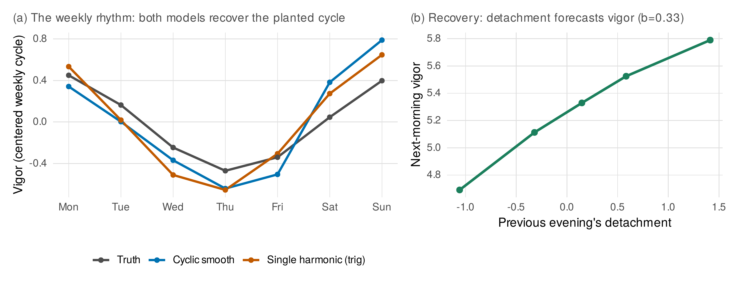
Note. Panel (a): the weekly vigor cycle recovered by a single trigonometric harmonic and by a cyclic spline, both tracking the planted truth (a mid-week trough, a weekend peak). The trigonometric model is efficient when the shape is a known sinusoid; the cyclic smooth is the theory-agnostic default. Panel (b): the within-person recovery effect, next-morning vigor rising with the previous evening’s psychological detachment, the recovery process at the heart of the stress-recovery literature.
Table 35.5. Cycle-Testing Decision Guide
| Approach | When it fits | What it assumes |
|---|---|---|
| Trigonometric harmonic | Theory predicts a smooth single-peak rhythm | A sinusoidal shape at the stated period |
| Cyclic spline | Shape unknown or possibly multi-peak | Smoothness and period closure only |
| Day-of-week dummies | No cyclical structure expected | Nothing, but discards the rhythm |
Note. The choice encodes a theoretical commitment about the rhythm’s shape. Fitting a flexible smooth when theory predicts a sinusoid wastes power; forcing a sinusoid when the shape is unknown risks misfit; using free dummies throws away the structure that is the phenomenon.
35.4.2 Recovery, Weekends, and Demands
The recovery hypothesis is that detaching from work in the evening restores the resources that the next day draws on, and it is a within-person lagged claim that the diary is built to test: regressing next-morning vigor on the previous evening’s psychological detachment, centered within person and crossing the night boundary with the care that Chapter 5 pressed, recovers a coefficient of 0.33 against a planted 0.35, so that a worker’s own better-than-usual detachment forecasts that worker’s own higher vigor. The weekend adds a discontinuity, not merely a low point on a smooth cycle but a genuine jump, and modeling it as a piecewise shift recovers a weekend vigor boost of 0.51 against a truth of 0.50, which Figure 35.10 displays as the within-week restoration it is. Job demands moderate the system as planted: workers reporting higher demands detach less, with a demands-detachment coefficient of \(-0.36\) against a truth of \(-0.30\), and report lower baseline vigor, so the recovery process that protects vigor is least available to the workers who need it most, a substantive finding the model surfaces. Finally, the day’s interruptions are a count, and a Poisson mixed model recovers their structure: interruptions rise with job demands, the log-rate coefficient being 0.51 against a truth of 0.50, and peak in the middle of the week, the count outcome handled by the generalized linear mixed model of Chapter 15 rather than forced into a linear mold.
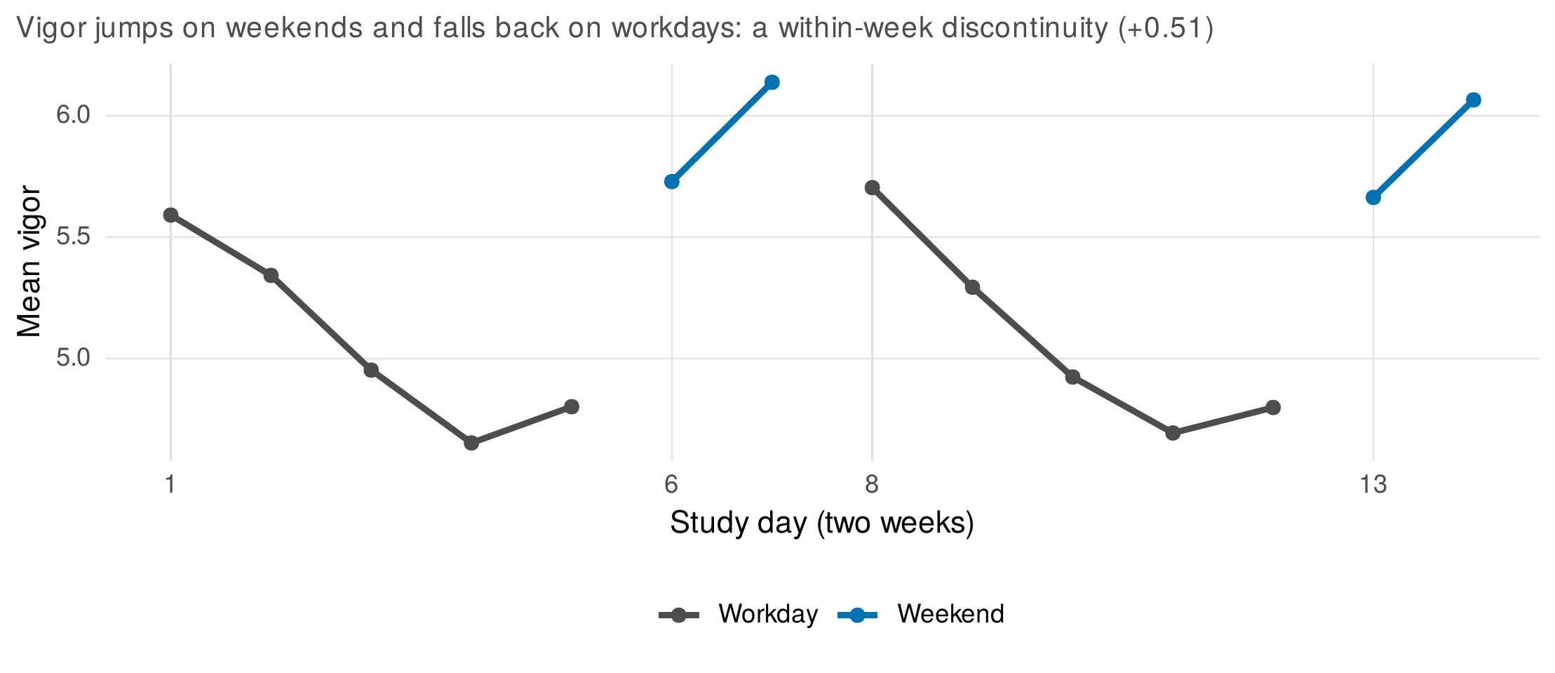
Note. Mean vigor across the two-week diary, with workdays and weekends distinguished. Vigor jumps on the weekend and falls back when the workweek resumes, a within-week discontinuity of about half a scale point that a piecewise model captures and a smooth weekly cycle would blur. The weekend is not merely the low-strain end of a gradient; it is a qualitatively different state.
In Practice • In Practice: organizational access and consent
Organizational diary research runs on access that is granted hierarchically and can be withdrawn, and the consent chain has a structure that individual research does not. An employer’s permission to study a workforce is not the employees’ consent to participate, and the two must be kept distinct, with participation voluntary and non-participation invisible to supervisors, or the data are coerced and the estimates biased by who dared to decline. Organizational data also carry the risk that within-person findings will be read as individual performance evaluations, so a study specifies in advance that its results will not be used to appraise particular employees, and it aggregates to protect individuals from a management that may be curious about single cases. The methods section that states these safeguards is not boilerplate; it is what makes the sample trustworthy.
35.5 Domain Synthesis
The three cases share a discipline and a set of recurring objections that a reviewer for these fields will raise. The discipline is that within-person structure is the object, that a distribution parameter, an actor effect, a recovery lag are all within-person quantities that must be estimated with the centering, the uncertainty propagation, and the causal caution their nature demands, and that summarizing them into a between-person or trait network without laundering their uncertainty is the standard the plug-in fallacy fails. The recurring objections are three. The first is the demand for an experiment, the reviewer who reads any within-person association as a causal claim and asks where the manipulation is; the honest answer is that these designs estimate within-person association and temporal prediction, which constrain causal hypotheses without establishing them, and that overclaiming influence from a partner effect or a lead-lag is the error the caution ledger exists to prevent. The second is the misreading of sample size, the reviewer who calls eighty couples or two hundred workers a small sample; the answer is level-specific power literacy, that the relevant sample for a within-person effect is the number of occasions times persons, that the between-person sample governs only the between-person effects, and that the design’s power must be assessed at the level of the estimand, as Chapter 4 sets out. The third is the dismissal of the rhythm or the weekday as a nuisance control, which mistakes the theory for noise. Table 35.6 collects the reporting obligations for these domains, including the translation of within-person findings into the language applied audiences use, and the anchor literatures orient the reader who would go deeper: the density-distribution program in Fleeson and in Fleeson and Jayawickreme, the dyadic canon in Kenny, Kashy, and Cook with the diary craft in Laurenceau and Bolger, and the recovery and organizational-sampling literatures in Sonnentag, in Sonnentag and Fritz, and in Beal and in Gabriel and colleagues. These are the domains where the within-person revolution began, and the craft they reward is the one this chapter has practiced: to model the process where it lives, and to say no more than the within-person data support.
Table 35.6. Domain Reporting Checklist and Within-Person Translation
| Element | What to report (and how to translate) |
|---|---|
| Distribution parameters | The location-scale estimates, their stability, and their uncertainty when used as predictors |
| Centering | The centering used, and the within- versus between-person effects kept separate |
| Dyadic structure | Distinguishability, the error structure, and the actor/partner/between decomposition |
| Causal language | Association and prediction, not influence, unless a design supports more |
| Level-specific N | Occasions and persons reported separately; power assessed at the estimand’s level |
| Translation | Within-person effects phrased as “on days when” or “for this person,” not as trait differences |
Note. The last row is the domain’s chronic communication task: a within-person effect describes variation within a person over time, and translating it into between-person trait language, which applied audiences expect, must be done without asserting a between-person difference the within-person data do not establish.
Chapter Summary
Social, personality, and organizational psychology are where within-person methods were born, and this chapter’s lesson is that their phenomena are within-person structure to be modeled with discipline. Case A treated personality as density distributions of states, estimating the person’s mean, variability, and reactivity as trait parameters, finding the mean highly stable and the higher-order parameters real but noisier, and insisting that a distribution parameter carried into a trait analysis brings its uncertainty with it, on pain of the attenuation the plug-in fallacy produces. Case B built the multilevel actor-partner model with the centering that separates the within-person actor and partner effects from the larger between-person association, recovering the planted structure and showing that grand-mean centering contaminates the actor effect, then estimated the common-fate growth and the asymmetric lead-lag with the caution that prediction is not influence. Case C tested the weekly cycle as theory rather than decoration, recovered the within-person recovery lag from evening detachment to next-morning vigor, modeled the weekend as a genuine discontinuity, and handled the interruption count with a Poisson mixed model. The synthesis is the domain’s reviewer playbook and its translation discipline: model the process where it lives, assess power at the estimand’s level, and say no more than the within-person data support.
Baird, B. M., Le, K., & Lucas, R. E. (2006). On the nature of intraindividual personality variability: Reliability, validity, and associations with well-being. Journal of Personality and Social Psychology, 90(3), 512–527. https://doi.org/10.1037/0022-3514.90.3.512
Beal, D. J. (2015). ESM 2.0: State of the art and future potential of experience sampling methods in organizational research. Annual Review of Organizational Psychology and Organizational Behavior, 2, 383–407. https://doi.org/10.1146/annurev-orgpsych-032414-111335
Bolger, N., Davis, A., & Rafaeli, E. (2003). Diary methods: Capturing life as it is lived. Annual Review of Psychology, 54, 579–616. https://doi.org/10.1146/annurev.psych.54.101601.145030
Bolger, N., DeLongis, A., Kessler, R. C., & Wethington, E. (1989). The contagion of stress across multiple roles. Journal of Marriage and the Family, 51(1), 175–183. https://doi.org/10.2307/352378
Butler, E. A. (2011). Temporal interpersonal emotion systems: The “TIES” that form relationships. Personality and Social Psychology Review, 15(4), 367–393. https://doi.org/10.1177/1088868311411164
Fleeson, W. (2001). Toward a structure- and process-integrated view of personality: Traits as density distributions of states. Journal of Personality and Social Psychology, 80(6), 1011–1027. https://doi.org/10.1037/0022-3514.80.6.1011
Fleeson, W., & Jayawickreme, E. (2015). Whole trait theory. Journal of Research in Personality, 56, 82–92. https://doi.org/10.1016/j.jrp.2014.10.009
Gabriel, A. S., Podsakoff, N. P., Beal, D. J., Scott, B. A., Sonnentag, S., Trougakos, J. P., & Butts, M. M. (2019). Experience sampling methods: A discussion of critical trends and considerations for scholarly advancement. Organizational Research Methods, 22(4), 969–1006. https://doi.org/10.1177/1094428118802626
Gistelinck, F., & Loeys, T. (2019). The actor-partner interdependence model for longitudinal dyadic data: An implementation in the SEM framework. Structural Equation Modeling: A Multidisciplinary Journal, 26(3), 329–347. https://doi.org/10.1080/10705511.2018.1527223
Ilies, R., Scott, B. A., & Judge, T. A. (2006). The interactive effects of personal traits and experienced states on intraindividual patterns of citizenship behavior. Academy of Management Journal, 49(3), 561–575. https://doi.org/10.5465/amj.2006.21794672
Kenny, D. A., Kashy, D. A., & Cook, W. L. (2006). Dyadic data analysis. Guilford Press.
Laurenceau, J.-P., Barrett, L. F., & Pietromonaco, P. R. (1998). Intimacy as an interpersonal process: The importance of self-disclosure, partner disclosure, and perceived partner responsiveness in interpersonal exchanges. Journal of Personality and Social Psychology, 74(5), 1238–1251. https://doi.org/10.1037/0022-3514.74.5.1238
Laurenceau, J.-P., & Bolger, N. (2005). Using diary methods to study marital and family processes. Journal of Family Psychology, 19(1), 86–97. https://doi.org/10.1037/0893-3200.19.1.86
Ledermann, T., & Kenny, D. A. (2012). The common fate model for dyadic data: Variations of a theoretically important but underutilized model. Journal of Family Psychology, 26(1), 140–148. https://doi.org/10.1037/a0026624
Reis, H. T., & Wheeler, L. (1991). Studying social interaction with the Rochester Interaction Record. Advances in Experimental Social Psychology, 24, 269–318. https://doi.org/10.1016/S0065-2601(08)60332-9
Sels, L., Ceulemans, E., & Kuppens, P. (2019). All’s well that ends well? A test of the peak-end rule in couples’ conflict discussions. European Journal of Social Psychology, 49(4), 794–806. https://doi.org/10.1002/ejsp.2547
Sonnentag, S. (2003). Recovery, work engagement, and proactive behavior: A new look at the interface between nonwork and work. Journal of Applied Psychology, 88(3), 518–528. https://doi.org/10.1037/0021-9010.88.3.518
Sonnentag, S., & Fritz, C. (2007). The Recovery Experience Questionnaire: Development and validation of a measure for assessing recuperation and unwinding from work. Journal of Occupational Health Psychology, 12(3), 204–221. https://doi.org/10.1037/1076-8998.12.3.204
Wheeler, L., & Reis, H. T. (1991). Self-recording of everyday life events: Origins, types, and uses. Journal of Personality, 59(3), 339–354. https://doi.org/10.1111/j.1467-6494.1991.tb00252.x
Wright, A. G. C., & Zimmermann, J. (2019). Applied ambulatory assessment: Integrating idiographic and nomothetic principles of measurement. Psychological Assessment, 31(12), 1467–1480. https://doi.org/10.1037/pas0000685