Chapter 3
Measurement Across Time and Timescales
A change score inherits every flaw of the measurements it is built from, and adds a few of its own. Before we ask whether a person changed, we must be able to defend a prior claim that is easy to assume and hard to earn: that the instrument meant the same thing on both occasions. This chapter is about that claim, and about what reliability means once measurements repeat.
Learning Objectives
After working through this chapter, you should be able to: (1) explain why the measurement-quality requirements for questions about level, change, and variability are different; (2) compute and interpret separate between-person and within-person reliabilities for an intensive longitudinal scale; (3) explain why a coefficient alpha computed on stacked repeated-measures data is uninterpretable; (4) write momentary items that respect a stated reference period and timescale; (5) define configural, metric, and scalar invariance conceptually and predict the consequences of their violation; (6) distinguish construct continuity from score comparability, including the case of heterotypic continuity; and (7) evaluate the reliability of change scores and of derived within-person variability indices.
3.1 What Must Stay the Same for Change to Be Interpretable
Imagine weighing yourself each morning on a bathroom scale and recording the numbers. If the scale is trustworthy, the sequence of numbers tells you about changes in your weight. But suppose that, unknown to you, the scale slowly loses calibration and reads two kilograms high by the end of the month. Now the rising sequence reflects the instrument, not your body, and the change you infer is an artifact. Or suppose the scale grows erratic, giving readings that jump around more and more from day to day even when your weight is stable. Now the numbers still center on the truth, but each one is less trustworthy than the last, and a difference between two of them could be mostly noise. Constructs in psychology are measured with instruments that can drift and degrade in exactly these ways, and the drift is rarely as visible as a miscalibrated scale.
Three distinct things must hold for a repeated measurement to yield an interpretable change, and Figure 3.1 illustrates each by showing a person whose true standing on some trait never changes. The first requirement is that the instrument measures the same construct at each occasion, so that the numbers refer to the same thing. The second is that it uses the same metric, so that a given score means the same amount of the construct at each occasion; Panel B of Figure 3.1 shows a metric that drifts upward, manufacturing the appearance of growth in a person who has not changed. The third is that it retains the same precision, so that scores are comparably trustworthy across occasions; Panel C shows precision degrading, so that later scores scatter more widely around the truth. These three requirements map, informally, onto the formal levels of measurement invariance introduced in Section 3.5 and developed fully in Chapter 18: same construct corresponds to configural invariance, same metric to metric and scalar invariance, and same precision to the equality of measurement error across time.
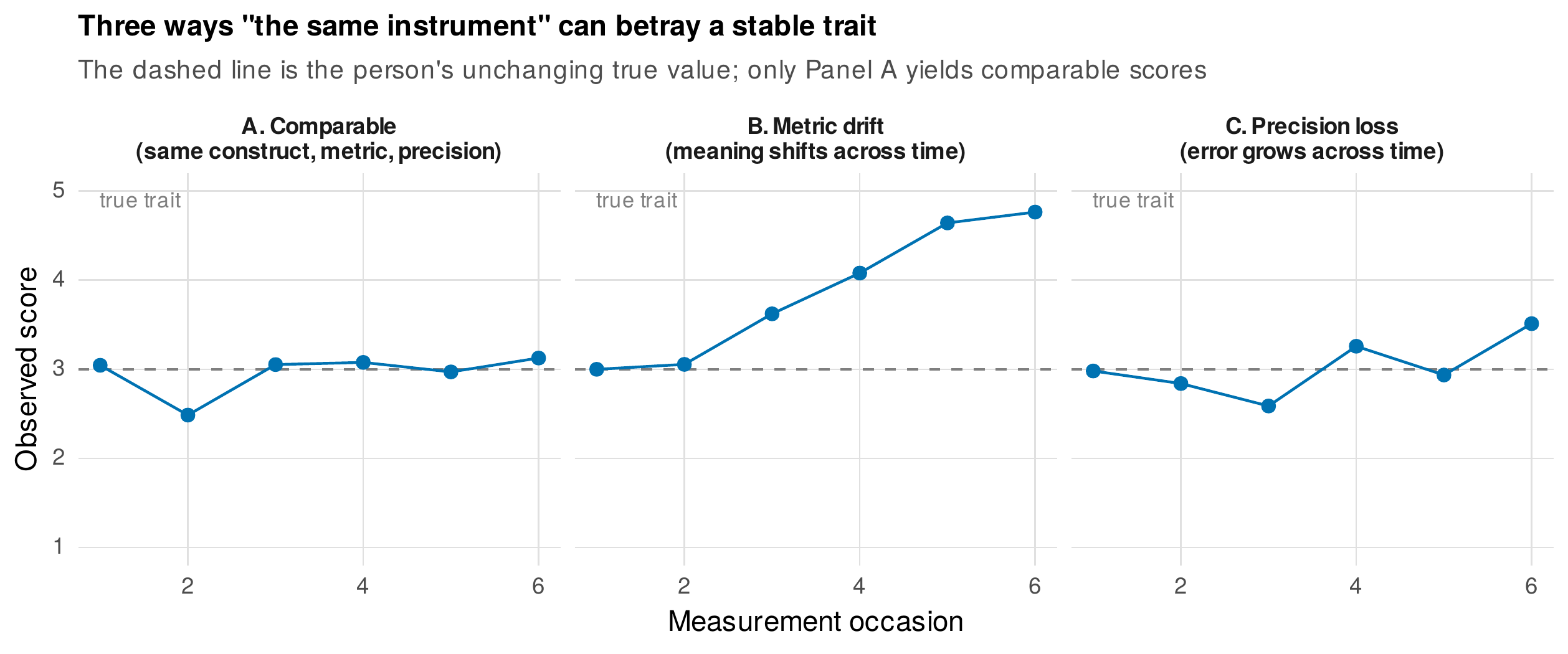
Note. Simulated data for a person whose true trait value (dashed line) is constant across six occasions. In Panel A the instrument is stable and the observed scores are comparable. In Panel B the metric drifts upward, producing apparent change where there is none. In Panel C precision degrades, so later scores are less trustworthy than earlier ones.
A subtler complication is that keeping the construct the same sometimes requires changing the items. Consider aggression across development. In a five-year-old it manifests as hitting, biting, and tantrums; in a fifteen-year-old the same underlying disposition manifests as verbal hostility, fighting, and rule violation. An instrument that asked about biting at both ages would measure the construct well at five and badly at fifteen. This is heterotypic continuity: the construct is continuous, but its behavioral indicators change with development, so that measuring the same construct demands different, age-appropriate items (Figure 3.2). Heterotypic continuity forces two design decisions. First, it argues for including anchor items, indicators that remain valid across the age range, to link the age-specific measures onto a common scale. Second, it means that raw-score comparability cannot be assumed and must be established analytically, through the longitudinal linking and partial-invariance methods of Chapter 18. The apparent stability or change in a construct can be an artifact of holding the items fixed when they should have shifted, or of shifting them without linking (Widaman, Ferrer, & Conger, 2010).
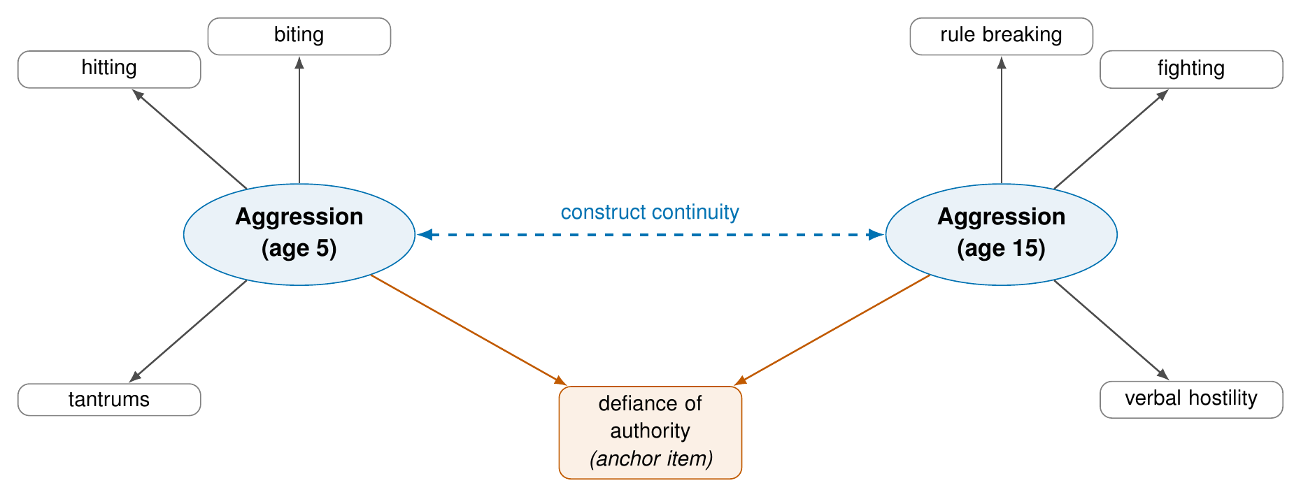
Note. The latent construct persists across age, but its behavioral indicators change. An anchor item valid at both ages (orange) provides the common reference needed to place the two age-specific measures on one scale.
3.2 Reliability When Measures Repeat
Classical test theory defines reliability as the proportion of observed-score variance that is true-score rather than error variance, and for a single cross-sectional measurement that definition is enough. Once measures repeat, a single reliability coefficient is no longer enough, because reliability is specific to a population and to a level of analysis. The same scale can be highly reliable for ranking persons on their average standing and poorly reliable for detecting a person’s momentary fluctuations, as the worked example of Section 3.3 will show concretely. A number such as “\(\alpha = .85\)” reported from one sample at one occasion licenses none of the repeated-measures uses without further evidence.
The most persistent piece of folklore in the measurement of change concerns the reliability of the difference score, and it is worth confronting directly because Chapter 10 will need it settled. The classical result, associated with Cronbach and Furby (1970), is that difference scores are often unreliable, and it is true as far as it goes.
Foundations Box • the reliability of a difference score
Let \(Y_1\) and \(Y_2\) be pretest and posttest scores with equal variance \(\sigma^2\) and equal reliability \(\rho\), and let \(\rho_{12}\) be their observed correlation. The difference is \(D = Y_2 - Y_1\). Its observed variance is
and the error variance in \(D\) is the sum of the two error variances, \(2(1-\rho)\sigma^2\). The reliability of the difference score is one minus the error-to-observed ratio:
The lesson people take from Equation (3.2) is alarming: as the pretest-posttest correlation \(\rho_{12}\) approaches the reliability \(\rho\), the reliability of the difference approaches zero. If two occasions correlate at \(.80\) and each is reliable at \(.80\), the difference is reliable at \(0\). But read the formula again with its meaning restored. A high \(\rho_{12}\) means people keep their rank order from pretest to posttest, that is, everyone changes by about the same amount, so there is little between-person variance in change for a reliability coefficient to detect. Low difference-score reliability signals homogeneous change, not invalid measurement. The difference score remains an unbiased estimate of each person’s within-person change; its low reliability is a statement about the precision with which individual differences in change can be detected, not about whether change occurred (Rogosa, Brandt, & Zimowski, 1982). This distinction, precision of individual-difference detection versus validity of the within-person quantity, recurs throughout the book.
A more honest framing than any single coefficient comes from generalizability theory, which treats an observed score as a sample from a universe of admissible observations and asks how much of its variance is attributable to each facet of measurement (Cronbach, Gleser, Nanda, & Rajaratnam, 1972). For repeated-measures data the relevant facets are persons, occasions, and items, crossed as in Figure 3.3. Generalizability theory decomposes the total variance of item responses into a component for stable person differences, a component for occasions within persons (real momentary states), a component for items, and their interactions and residual. The value of this framing is that it refuses to answer “how reliable is the scale?” in the abstract and instead forces the question “reliable for what, generalizing over what?” Reliability for ranking persons generalizes over occasions and items and lives in the person component; reliability for detecting momentary states generalizes over items only and lives in the person-by-occasion component. The two draw on different pieces of the same variance decomposition, which is why they can diverge so sharply.
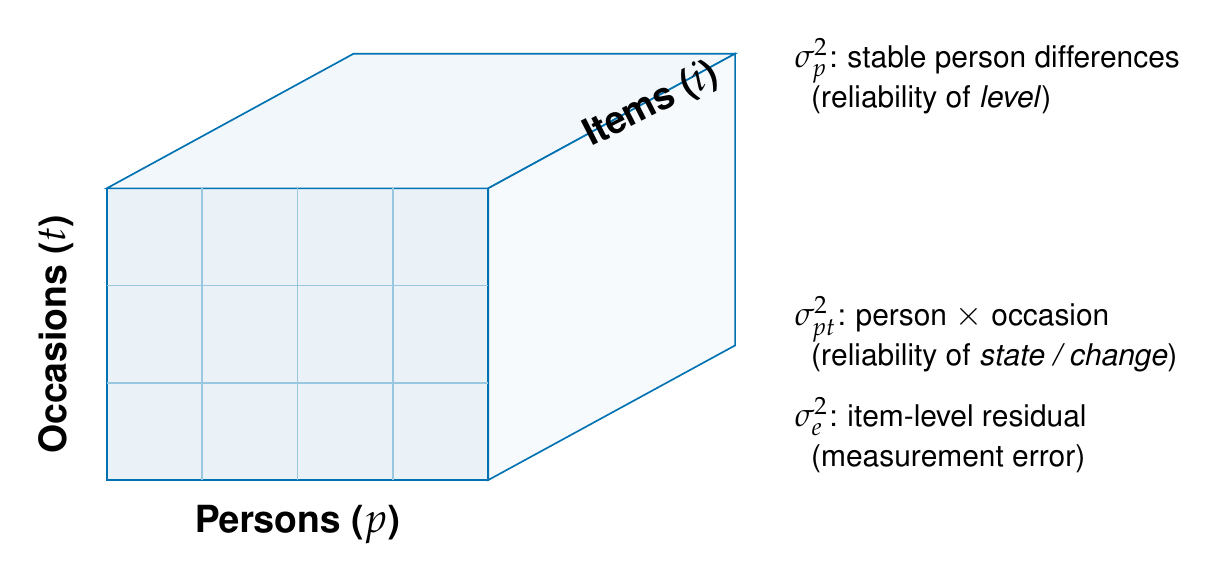
Note. Each cell is one item response from one person on one occasion. Generalizability theory partitions the total variance into components for persons, occasions within persons, items, and their interactions. Different reliability questions draw on different components: the between-person component governs the reliability of a person’s average level, the person-by-occasion component governs the reliability of momentary states.
3.3 Multilevel Reliability for Intensive Data
Intensive longitudinal data make the level-specificity of reliability unavoidable, because each person contributes many occasions and the item structure can differ between the person and occasion levels. The framework developed by Cranford and colleagues (2006) and by Geldhof, Preacher, and Zyphur (2014) formalizes two reliabilities that every intensive longitudinal scale possesses simultaneously. Between-person reliability asks how dependably the scale ranks persons on their average level, aggregating over their many occasions; it is high when stable person differences are large relative to error. Within-person reliability asks how dependably the scale detects a person’s momentary deviation from their own average at a single occasion; it is high when momentary state variance is large relative to item-level error. These are different quantities, and a scale can excel at one while failing at the other.
The worked example uses the four negative-affect items in the book’s affect_ema_items companion dataset, the item-level responses whose average is the momentary negative-affect composite of affect_ema. Decomposing the variance of these items with a crossed random-effects model yields a between-person (stable) variance of about \(0.17\), a person-by-occasion (momentary state) variance of about \(0.15\), and an item-level residual of about \(0.53\). From these components, the between-person reliability of a person’s average level, computed over an average of sixty-one occasions and four items, is about \(.97\): with sixty-one momentary reports, a person’s average negative affect is estimated with great precision. The within-person reliability of a single momentary composite, by contrast, is only about \(.53\): one four-item report is a noisy indicator of where a person sits, at that moment, relative to their own norm. A multilevel factor analysis tells the same story in the language of omega: the between-person omega for the negative-affect scale is about \(.88\), whereas the within-person omega is about \(.61\). The items cohere well as a scale when we compare people’s averages, and much less well when we track a single person’s fluctuations. This discrepancy is not a defect of this particular scale; it is the normal state of affairs, and it is invisible to anyone who reports a single reliability coefficient.
Common Pitfall • coefficient alpha on stacked long data
A tempting shortcut, when intensive longitudinal data sit in long format with one row per person-occasion, is to run coefficient alpha on the stacked item columns, ignoring the person structure. For the negative-affect items above, this pooled alpha is about \(.71\), a number that looks respectable and means almost nothing. It is a blend of the between-person reliability (\(\approx .88\)) and the within-person reliability (\(\approx .61\)), weighted by the sample’s ratio of between to within variance, and it corresponds to neither quantity a researcher would actually want. Reporting it invites readers to assume the scale is equally good for level and for change, which it is not. The correct practice is to decompose reliability by level and report both, using a multilevel CFA or the generalizability-theory coefficients; the pooled alpha should never appear. A related error is to report the within-person omega alone and describe it as “the scale’s reliability,” as though it were a global property, when it is specifically the reliability of momentary deviations and says nothing about the reliability of person averages.
Two practical questions follow. The first is how many items a momentary scale needs. Because per-prompt burden is precious (Chapter 2), momentary scales are short, and the within-person reliability formula shows why this hurts: halving the number of items raises the item-level error contribution to each momentary score. There is no universal minimum, but within-person reliability, not between-person reliability, should drive the decision, because the between-person reliability of aggregates is buoyed by the sheer number of occasions and will look adequate almost regardless. The second question is whether a single item can serve. Single-item momentary measures are defensible when the construct is narrow and concrete, when burden is binding, and when there is within-person validity evidence, but a single item’s within-person reliability cannot be estimated from internal consistency at all and must be established by other means, such as a planned occasional multi-item probe or test-retest over short intervals (Schuurman & Hamaker, 2019). Table 3.1 organizes the coefficients this section has introduced.
Table 3.1. Reliability coefficients for repeated-measures data.
| Coefficient | Question it answers | How to obtain it |
|---|---|---|
| Between-person reliability (omega-between; \(R_{kF}\)) | How dependably does the scale rank persons on their average level? | Two-level CFA (between omega); variance components |
| Within-person reliability (omega-within; \(R_{kR}\)) | How dependably does a single report detect a momentary deviation? | Two-level CFA (within omega); variance components |
| Reliability of the person mean | How stable is a person’s estimated average, given \(T\) occasions? | \(\sigma^2_p / (\sigma^2_p + \sigma^2_{w}/T)\) |
| Reliability of a difference score | How precisely are individual differences in change detected? | \((\rho - \rho_{12})/(1 - \rho_{12})\) from test-retest |
| Reliability of iSD / inertia | How dependably is within-person variability or dynamics estimated? | Simulation or split-half; grows slowly with \(T\) |
Note. The between- and within-person coefficients follow the multilevel framework of Cranford et al. (2006) and Geldhof et al. (2014); \(\sigma^2_w\) denotes the occasion-level variance of the composite. R implementations are shown in Section 3.8.
3.4 Item and Scale Design for Momentary Assessment
Measurement quality is designed in before it is estimated, and momentary assessment imposes design constraints that trait measurement does not. The single most important is the reference period. A momentary item must ask about the present or the recent, bounded interval, “right now” or “since the last prompt,” because the entire rationale of intensive sampling is to capture experience before memory reconstructs it (Chapter 2). An item that asks “over the past week, how tense have you been?” embedded in a momentary protocol is a retrospective summary in disguise; it reintroduces exactly the recall bias the design was meant to defeat, and it confuses the timescale, since a weekly summary cannot vary from prompt to prompt within a day. Figure 3.4 contrasts a well-formed momentary item with a poorly formed one that smuggles a retrospective window into a momentary study.
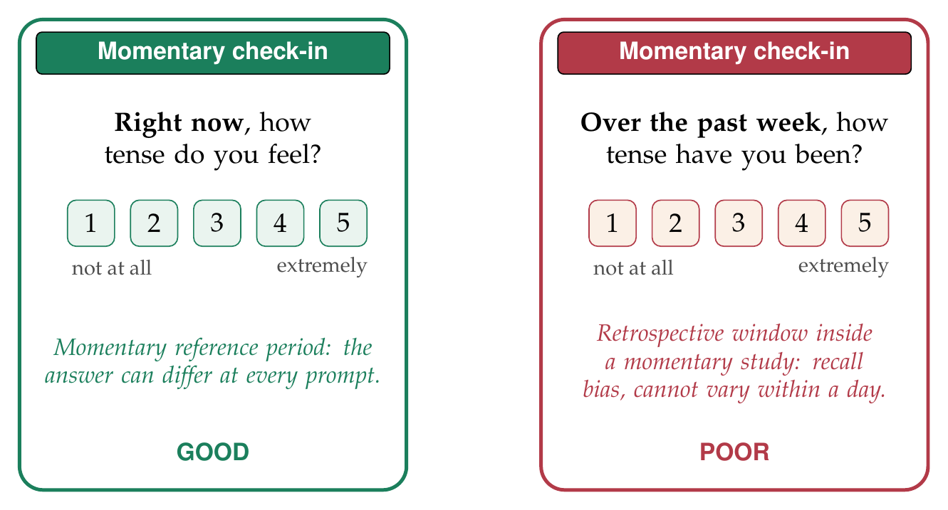
Note. Mock-ups. The reference period is the decisive design choice: a momentary item must ask about the present or the interval since the last prompt, so that responses can vary across the day and are not reconstructed from memory.
Beyond the reference period, several choices shape momentary data quality. Response scales should be consistent across prompts, whether visual analog scales, which capture fine gradations but demand more of the respondent, or a small number of Likert categories, which are faster and more robust at high frequency; mixing formats across prompts undermines comparability. Items can be rotated across prompts, with a fixed core measured every time and a rotating periphery measured occasionally, a form of planned missingness that reduces burden at the cost of analysis complexity (Chapter 6). Momentary versions of standard instruments are widely used, and Table 3.2 lists common adaptations; the essential discipline is to adapt the reference period and wording from a validated trait instrument and to cite the specific momentary version used rather than assume the trait scale’s psychometrics transfer. Table 3.3 collects the design rules into a checklist.
Table 3.2. Momentary adaptations of common self-report constructs (illustrative).
| Trait construct | Momentary adaptation | Reference period |
|---|---|---|
| Positive / negative affect (PANAS tradition) | Momentary affect adjectives (e.g., tense, upset, content, cheerful) | “right now” |
| Perceived stress | Momentary stress appraisal item(s) | “right now” or “since last prompt” |
| Self-esteem | State self-esteem (e.g., “right now I feel good about myself”) | “right now” |
| Rumination | Momentary repetitive thought | “since the last prompt” |
Note. Wordings are illustrative, not endorsed instruments. Adapt from a validated trait scale and cite the specific momentary version used; do not assume the trait scale’s reliability and validity transfer to the momentary level.
Table 3.3. A checklist for writing momentary items.
| Do | Avoid |
|---|---|
| State an explicit momentary reference period (“right now”) | Retrospective windows (“over the past week”) inside a momentary protocol |
| Measure one construct per item | Double-barreled items (“tense and worried”) |
| Keep the response scale identical across prompts | Mixing visual-analog and Likert formats across prompts |
| Fix a small core item set; rotate the rest | Long, unchanging item batteries that fatigue respondents |
| Randomize order where order effects are plausible | Fixed order that lets earlier items prime later ones |
| Cite the specific momentary version and its evidence | Assuming the trait scale’s psychometrics transfer |
Note. The checklist operationalizes the design principles of Chapter 2 at the level of the individual item.
3.5 Measurement Invariance: The Concept
Measurement invariance is the formal machinery for the “same metric” requirement of Section 3.1, and although its full apparatus waits for Chapter 18, its logic can be grasped as a ladder, shown in Figure 3.5. Each rung holds one more feature of the measurement model equal across occasions, and each licenses one more kind of comparison. At the bottom, configural invariance requires only that the same items load on the same factor in the same pattern at every occasion; it establishes that the same construct is being measured, but licenses no quantitative comparison. The next rung, metric (or weak) invariance, adds equal factor loadings across time; because the metric of the latent variable is now constant, it licenses comparing the construct’s associations with other variables over time and comparing the slopes of change. The third rung, scalar (or strong) invariance, adds equal item intercepts; only now are the latent means comparable across occasions, which means that only at this rung is a claim about growth in the level of the construct defensible. The top rung, strict (or residual) invariance, adds equal residual variances, so that even observed-score reliabilities are equal across time; it is rarely required for substantive conclusions. Table 3.4 states what each rung licenses and what it does not.
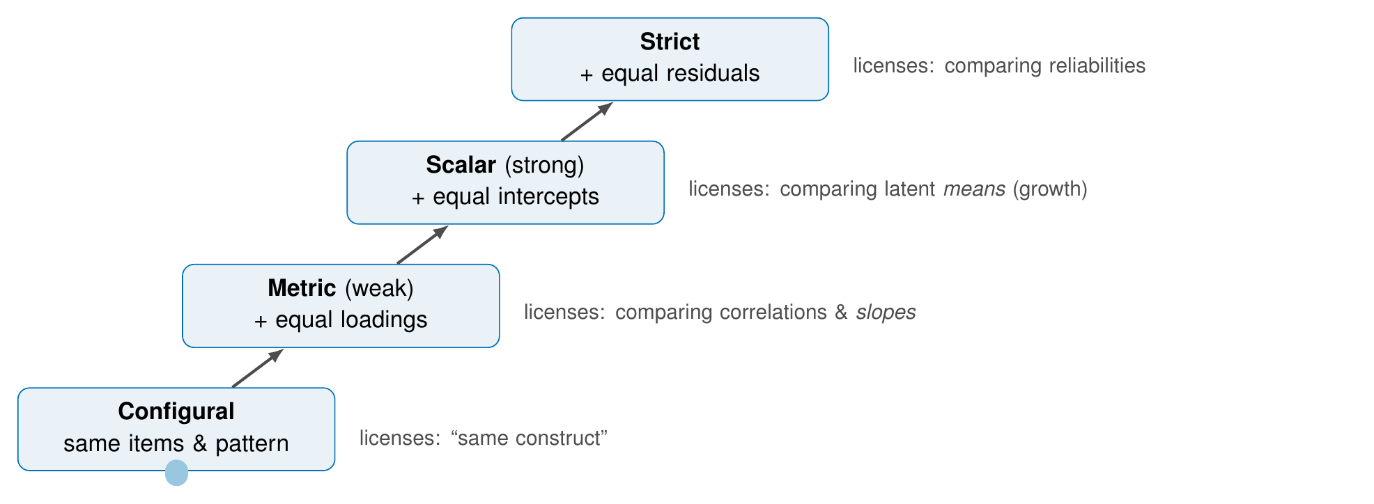
Note. Conceptual figure; the corresponding equations and tests appear in Chapter 18. Higher rungs subsume lower ones. The rung a study reaches determines which comparisons across time are defensible.
Table 3.4. Invariance levels and the comparisons they license.
| Level | Held equal across time | Licenses | Still unsafe |
|---|---|---|---|
| Configural | Item-factor pattern | “The same construct is measured” | Any quantitative comparison |
| Metric (weak) | + Factor loadings | Comparing associations and change slopes | Comparing latent means |
| Scalar (strong) | + Item intercepts | Comparing latent means (growth in level) | – |
| Strict | + Residual variances | Comparing observed reliabilities directly | – |
Note. Each level subsumes those above it in the table. Scalar invariance is the practical threshold for interpreting change in the mean level of a construct.
Longitudinal noninvariance arises for reasons peculiar to repeated measurement. Respondents may reinterpret items as they develop, so that a child and an adolescent read the same words differently. Panel conditioning (Chapter 2) can shift how seasoned respondents use a scale. A change of measurement mode, from paper to smartphone application, can alter item functioning. And the context of assessment, a lab at baseline versus daily life at follow-up, can change what an item captures. The consequence of ignoring noninvariance is not merely inelegant: when loadings or intercepts drift and are assumed equal, estimates of growth are biased, and a study can report change in a construct that is really change in the instrument. Crucially, this bias is not confined to structural equation models. A researcher who avoids invariance testing by fitting a multilevel growth model to sum scores has not escaped the problem; the sum score simply assumes strict invariance without testing it, and inherits the bias silently. There is no free lunch by switching analytic frameworks, a point Chapter 18 demonstrates with a simulation.
3.6 Reliability and Validity of Derived Within-Person Indices
Intensive longitudinal research increasingly treats features of a person’s time series as scores in their own right: the within-person standard deviation (iSD) as a measure of emotional variability, the root mean square of successive differences (RMSSD) as a measure of instability, and the lag-one autocorrelation (inertia) as a measure of emotional persistence (these indices are developed in Chapter 7). Because these are estimated from a person’s series, their reliability depends heavily on the number of occasions, and far more than the reliability of a simple mean does. Figure 3.6 shows, by simulation, how the reliability of three quantities grows with the number of occasions per person. A person’s mean is already reliable at around \(.70\) with only four occasions and exceeds \(.95\) by sixty. The within-person standard deviation reaches acceptable reliability more slowly, passing \(.70\) only around fourteen occasions. Inertia, the autocorrelation, is the most demanding: at fourteen occasions its reliability is only about \(.34\), and it approaches \(.80\) only near sixty occasions. A two-week diary with one prompt per day, which yields a reliable estimate of a person’s average, yields a barely usable estimate of that person’s emotional inertia. Reporting inertia from short series without acknowledging its unreliability is a common and consequential error.
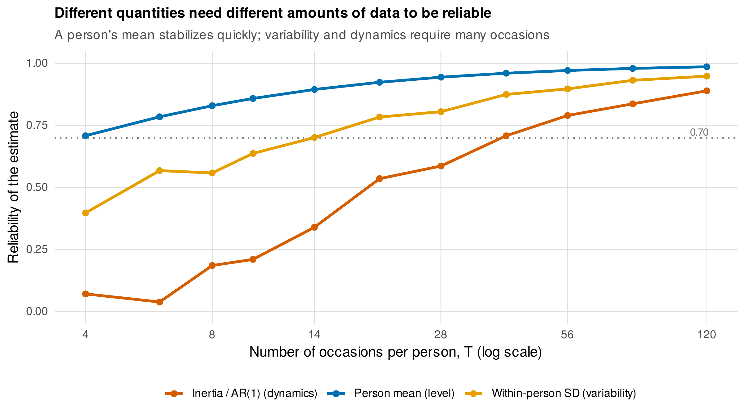
Note. Simulation. The person mean (blue) becomes reliable with few occasions; the within-person standard deviation (orange) requires more; the lag-one autocorrelation, or inertia (red), requires many. The dotted line marks a reliability of \(.70\). Both axes concern occasions per person, not sample size.
A second hazard specific to variability indices is their entanglement with the mean. For any bounded response scale, the range of possible variation is constrained by the level: a person whose momentary negative affect hovers near the floor of the scale simply cannot exhibit as large a standard deviation as a person near the middle, so an observed association between mean and variability can be a mathematical artifact of the bounds rather than a substantive finding (Mestdagh et al., 2018). This matters because emotional variability is often studied as a correlate of psychopathology, and if higher symptom levels come with higher means, an apparent link between variability and symptoms may be the mean masquerading as variability. The remedies are to use a mean-corrected variability index such as the relative variability index, to control for the mean explicitly, or, better, to move to the model-based approach of Chapter 16, which estimates within-person variance as a parameter while adjusting for the mean. The broader caution, argued forcefully by Dejonckheere and colleagues (2019), is that complex dynamic indices often add little predictive information beyond the mean and the variance, and their unreliability at realistic series lengths is part of why. Figure 3.7 makes the level-specificity of structure vivid from another angle, comparing the between-person and within-person correlations among momentary affect items.
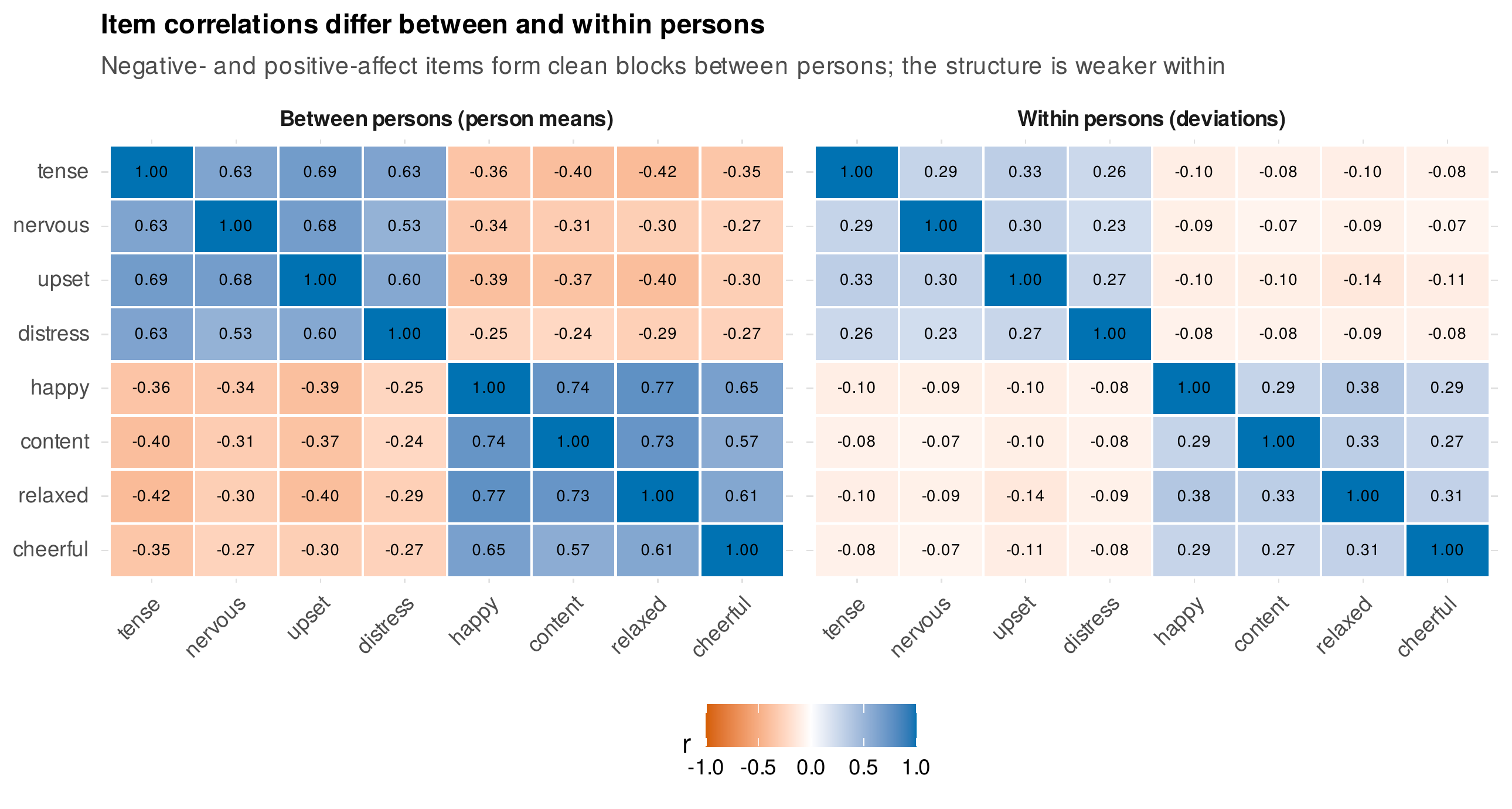
Note. Correlations among eight momentary affect items in affect_ema_items, computed between persons (left, from person means) and within persons (right, from person-centered deviations). Between persons the negative- and positive-affect items form clean, strongly correlated blocks; within persons the same blocks are much weaker, which is why between- and within-person reliabilities diverge.
3.7 Beyond Self-Report
Not all measurement across time is self-report. Actigraphy records movement and estimates sleep; ambulatory physiology records heart rate and its variability; smartphone and wearable sensors log location, activity, and communication (Chapter 2). These channels escape some problems of self-report, notably reactivity and recall, but they do not escape measurement theory; they relocate it. For passive and physiological measures, the crucial measurement decisions move upstream into synchronization and preprocessing: aligning streams sampled at different rates onto a common clock, deciding an epoch length over which to aggregate, defining artifacts and how to handle them, and choosing features to extract from a raw signal. Each of these is a measurement choice with reliability and validity consequences as real as item wording, and each should be reported and, ideally, tested for robustness. Validity evidence for passive measures also takes a particular form: because a sensor-derived index such as “time at home” is a proxy for a psychological construct such as withdrawal, its validity rests on the strength of that proxy relationship, which must be established rather than assumed (Fried, Flake, & Robinaugh, 2022). The measurement principles of this chapter, same construct, same metric, same precision, and level-specific reliability, apply to a stream of accelerometer counts exactly as they apply to a mood item, even though the techniques for establishing them differ.
3.8 Estimating Reliability in R
The reliabilities discussed above are computable with a few lines of R, and seeing the computation makes their meaning concrete. The worked example uses the four negative-affect items in affect_ema_items. The first task is the variance decomposition that underlies the generalizability-theory reliabilities, obtained by stacking the items into long form and fitting a crossed random-effects model with random effects for persons, for occasions within persons, and for items.
library(lme4)
d <- readRDS("Examples/data/affect_ema_items.rds")
na_items <- c("na_tense", "na_nervous", "na_upset", "na_distressed")

# Stack items into long form: one row per person x occasion x item
long <- reshape(d[, c("person","day","beep", na_items)], varying = na_items,
                v.names = "resp", timevar = "item", times = na_items,
                direction = "long")
long <- long[!is.na(long$resp), ]
long$occ <- interaction(long$person, long$day, long$beep, drop = TRUE)

vc <- as.data.frame(VarCorr(lmer(resp ~ 1 + (1|person) + (1|occ) + (1|item),
                                 data = long)))
s2_p  <- vc$vcov[vc$grp == "person"]     # between-person   ~ 0.17
s2_pt <- vc$vcov[vc$grp == "occ"]        # within (state)   ~ 0.15
s2_e  <- vc$vcov[vc$grp == "Residual"]   # item-level error ~ 0.53

k <- 4; Tbar <- mean(tapply(!is.na(d$na_tense), d$person, sum))   # ~ 61
RkR <- s2_pt / (s2_pt + s2_e / k)                          # within  ~ 0.53
RkF <- s2_p  / (s2_p + s2_pt/Tbar + s2_e/(Tbar*k))         # between ~ 0.97
The second task computes the between- and within-person omega directly from a two-level confirmatory factor analysis, which many readers will find more familiar. The lavaan syntax specifies one factor at the within level and one at the between level, and omega is computed from the resulting loadings and residual variances at each level.
library(lavaan)
model <- "
  level: 1
    fw =~ na_tense + na_nervous + na_upset + na_distressed
  level: 2
    fb =~ na_tense + na_nervous + na_upset + na_distressed
"
fit <- sem(model, data = d, cluster = "person", missing = "listwise")

# omega at a level = (sum loadings)^2 * factor var /
#                    [ (sum loadings)^2 * factor var + sum residual vars ]
# Extract with parameterEstimates(fit); here: omega_within ~ .61, omega_between ~ .88
Running these confirms the numbers reported in Section 3.3: a between-person reliability near \(.97\) for the person average and a within-person reliability near \(.53\) for a momentary score, or, in omega terms, \(.88\) between and \(.61\) within. For contrast, the tempting but wrong pooled alpha, psych::alpha(d[na_items]), returns about \(.71\), the uninterpretable blend warned against above. The discipline the code enforces is that one must choose a level before computing a reliability, because there is no single number that describes the scale.
3.9 Reporting Reliability for Repeated Measures
Reviewers of intensive longitudinal work now expect reliability to be reported at the level that matches each claim, and a Method section that reports a single alpha will draw a query. The counterpart of the reporting discipline introduced in earlier chapters has four elements for reliability. First, report the reliability that matches the estimand: if the analysis concerns between-person differences in average level, report between-person reliability; if it concerns within-person fluctuation or coupling, report within-person reliability; if both, report both. Second, name the method and the model: state whether the coefficients come from a multilevel CFA or from generalizability-theory variance components, and give the software and version. Third, for derived indices such as iSD or inertia, report or acknowledge their reliability given the achieved number of occasions, rather than presenting them as if they were as dependable as a mean. Fourth, when a single-item momentary measure is used, state the basis for trusting it, since internal-consistency reliability is undefined for one item.
A model sentence, drawing these together for the negative-affect scale of the worked example, reads: “Reliability of the four-item momentary negative-affect scale was estimated in a two-level confirmatory factor analysis (lavaan 0.6-x). Between-person reliability (omega-between) was \(.88\), indicating that persons’ average levels were dependably distinguished; within-person reliability (omega-within) was \(.61\), indicating that a single momentary report distinguished occasions within a person only modestly. Because the primary analyses concern within-person coupling, the within-person coefficient is the relevant one, and its modest value is reflected in the attenuation corrections applied in Chapter 25.” Every clause names a level, and no clause offers a reliability coefficient without saying reliability of what.
Software Note • computing multilevel reliability
Several tools compute the coefficients of this chapter, and they agree when specified equivalently. In R, lavaan fits the two-level CFA from which between- and within-person omega are computed, and the semTools function for composite reliability supports multilevel models directly; the psych function multilevel.reliability (mlr) implements the Cranford and Shrout-Lane generalizability coefficients (\(R_{kF}\), \(R_{kR}\), and relatives), though on large numbers of occasions its internal model can fail to converge, in which case computing the coefficients from lme4 variance components, as in Section 3.8, is the robust fallback. The misty package offers convenience wrappers. In Mplus, the same two-level CFA is specified with TYPE = TWOLEVEL and the model constraint facility computes omega at each level. Whatever the tool, report which coefficient, at which level, from which model.
3.10 Common Misconceptions
Four beliefs recur. First, that an alpha above \(.70\) once justifies a scale forever and at every level: reliability is specific to a population, an occasion, and a level of analysis, and a between-person alpha says nothing about within-person reliability (Section 3.3). Second, that difference scores are inherently unreliable, so change scores should never be used: low difference-score reliability signals homogeneous change, not invalid measurement, and the change score remains an unbiased within-person quantity (the Foundations box; Rogosa et al., 1982). Third, that invariance testing is a structural-equation-modeling nicety that multilevel modelers can skip: fitting a growth model to sum scores assumes strict invariance without testing it and inherits the same bias, so switching frameworks buys no exemption. Fourth, in answer to the frequent question “can I use one item per construct in intensive assessment?”: sometimes, when the construct is narrow, burden is binding, and within-person validity evidence exists, but a single item’s within-person reliability cannot be read off internal consistency and must be established another way.
Chapter Summary
A change score is interpretable only if the instrument kept the same construct, the same metric, and the same precision across occasions (Figure 3.1), and sometimes keeping the construct the same requires changing the items, as in heterotypic continuity. Reliability, once measures repeat, is not one number: the same scale has a between-person reliability for ranking persons’ averages and a within-person reliability for detecting momentary states, and these routinely diverge, as the worked example’s \(.88\) versus \(.61\) shows. Coefficient alpha on stacked long data blends the two and means neither. Difference-score reliability, long maligned, reflects the homogeneity of change rather than the invalidity of measurement. Measurement invariance formalizes the “same metric” requirement as a ladder whose rungs license progressively stronger comparisons, and its violation biases growth estimates in multilevel and structural-equation frameworks alike. Derived within-person indices such as variability and inertia are scores whose reliability depends steeply on the number of occasions and which can be confounded with the mean. Report reliability at the level that matches the claim.
Where to Go Next
The threads of this chapter run forward throughout the book. The derived indices previewed here are developed in Chapter 7; the rehabilitation of the difference score prepares the two-occasion methods of Chapter 10; the model-based treatment of within-person variance is Chapter 16; the formal machinery of measurement invariance, with equations and a bias simulation, is Chapter 18; the consequences of measurement error for estimates of dynamics are Chapter 25; and the linking of age-specific measures under heterotypic continuity returns in the developmental applications of Chapter 34. The chapter’s single imperative is to state, for every reliability and every comparison, the level and the timescale at which it holds.
Exercises
- 3.1 Two reliabilities. Using
affect_ema_items, compute the between-person and within-person reliability of the four positive-affect items, following Section 3.8. Interpret the divergence, and state which coefficient you would report for a study of momentary positive-affect dynamics. - 3.2 Rewrite the items. Take three retrospective questionnaire items from any published trait scale and rewrite each as a momentary item with an explicit reference period. Justify each reference-period choice against Table 3.3.
- 3.3 Difference-score algebra. Derive Equation (3.2) from the definitions. Then compute the difference-score reliability for \(\rho = .85\) and \(\rho_{12} = .80\), and write two sentences explaining to a skeptical reviewer why a study using this change score is nonetheless informative.
- 3.4 Invariance threats. You are handed a twenty-year panel study of self-esteem measured from adolescence to midlife with the same questionnaire. Identify three plausible sources of longitudinal noninvariance and, for each, the comparison it would jeopardize.
- 3.5 Reliability and \(T\) (simulation). Adapt the simulation in
ch03_figures_V01.Rto estimate the reliability of the lag-one autocorrelation as a function of the number of occasions. At what series length does it reach \(.70\)? What does your answer imply for a two-week daily diary?
References
Cranford, J. A., Shrout, P. E., Iida, M., Rafaeli, E., Yip, T., & Bolger, N. (2006). A procedure for evaluating sensitivity to within-person change: Can mood measures in diary studies detect change reliably? Personality and Social Psychology Bulletin, 32(7), 917–929. https://doi.org/10.1177/0146167206287721
Cronbach, L. J., & Furby, L. (1970). How we should measure “change”: Or should we? Psychological Bulletin, 74(1), 68–80. https://doi.org/10.1037/h0029382
Cronbach, L. J., Gleser, G. C., Nanda, H., & Rajaratnam, N. (1972). The dependability of behavioral measurements: Theory of generalizability for scores and profiles. Wiley.
Dejonckheere, E., Mestdagh, M., Houben, M., Rutten, I., Sels, L., Kuppens, P., & Tuerlinckx, F. (2019). Complex affect dynamics add limited information to the prediction of psychological well-being. Nature Human Behaviour, 3(5), 478–491. https://doi.org/10.1038/s41562-019-0555-0
Fried, E. I., Flake, J. K., & Robinaugh, D. J. (2022). Revisiting the theoretical and methodological foundations of depression measurement. Nature Reviews Psychology, 1(6), 358–368. https://doi.org/10.1038/s44159-022-00050-2
Geldhof, G. J., Preacher, K. J., & Zyphur, M. J. (2014). Reliability estimation in a multilevel confirmatory factor analysis framework. Psychological Methods, 19(1), 72–91. https://doi.org/10.1037/a0032138
Horn, J. L., & McArdle, J. J. (1992). A practical and theoretical guide to measurement invariance in aging research. Experimental Aging Research, 18(3), 117–144. https://doi.org/10.1080/03610739208253916
Meredith, W. (1993). Measurement invariance, factor analysis and factorial invariance. Psychometrika, 58(4), 525–543. https://doi.org/10.1007/BF02294825
Mestdagh, M., Pe, M., Pestman, W., Verdonck, S., Kuppens, P., & Tuerlinckx, F. (2018). Sidelining the mean: The relative variability index as a generic mean-corrected variability measure for bounded variables. Psychological Methods, 23(4), 690–707. https://doi.org/10.1037/met0000153
Nezlek, J. B. (2017). A practical guide to understanding reliability in studies of within-person variability. Journal of Research in Personality, 69, 149–155. https://doi.org/10.1016/j.jrp.2016.06.020
Rogosa, D. R., Brandt, D., & Zimowski, M. (1982). A growth curve approach to the measurement of change. Psychological Bulletin, 92(3), 726–748. https://doi.org/10.1037/0033-2909.92.3.726
Schuurman, N. K., & Hamaker, E. L. (2019). Measurement error and person-specific reliability in multilevel autoregressive modeling. Psychological Methods, 24(1), 70–91. https://doi.org/10.1037/met0000188
Widaman, K. F., Ferrer, E., & Conger, R. D. (2010). Factorial invariance within longitudinal structural equation models: Measuring the same construct across time. Child Development Perspectives, 4(1), 10–18. https://doi.org/10.1111/j.1750-8606.2009.00110.x
Willett, J. B. (1988). Questions and answers in the measurement of change. Review of Research in Education, 15, 345–422. https://doi.org/10.3102/0091732X015001345