Chapter 4
Planning Longitudinal Studies: Power, Precision, and Design Trade-Offs
Chapter 2 chose designs and Chapter 3 secured their measurement. This chapter asks the question a grant panel will ask next: how large must the study be? For longitudinal models the honest answer is never a single number, because a study that is generously powered to estimate an average trajectory can be helpless to detect the individual differences in that trajectory. Planning means deciding which estimand matters and building the study around it, and the tool that makes this possible for realistic models is simulation.
Learning Objectives
After working through this chapter, you should be able to: (1) identify the design factors that drive power in repeated-measures ANOVA, multilevel growth, latent growth, and intensive longitudinal designs; (2) apply closed-form power for simple repeated designs and state where the formulas break down; (3) build a simulation-based power analysis for a longitudinal model from scratch, following a reusable six-step workflow; (4) use existing tools such as simr and Monte Carlo facilities for standard cases; (5) reason quantitatively about the trade-off between number of persons and number of occasions for a fixed budget; (6) plan for realistic attrition and compliance; and (7) justify a sample size to a grant panel in estimand-first, precision-aware language.
4.1 What Power Means When Models Have Many Parameters
In a two-group comparison, power is a single number attached to a single effect. A longitudinal model estimates many quantities at once, and each has its own power. Figure 4.1 makes the point with a single daily-diary design of thirty persons measured for fourteen days. In that one study, the variance of the random intercepts is detected with power essentially equal to one, the within-person effect of a daily predictor is detected with power about \(.82\), but the between-person effect, the cross-level interaction, and the variance of the random slopes are each detected with power near \(.50\), well below the conventional \(.80\). The same data collection is simultaneously overpowered and underpowered depending on the question. There is no such thing as “the power of this study”; there is only the power for a named estimand.
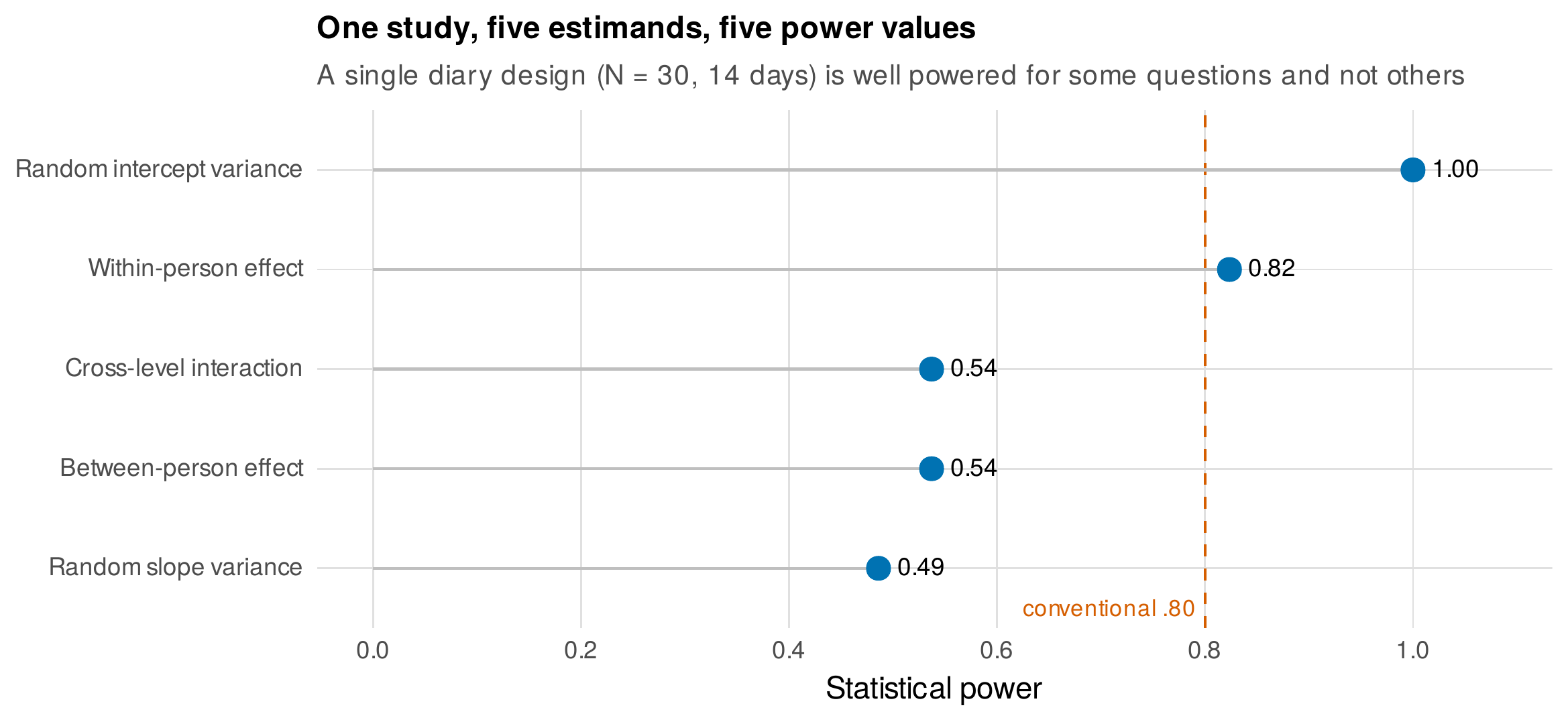
Note. Simulated power for five quantities estimated by the same multilevel model in a single daily-diary design (30 persons, 14 days). Power ranges from near \(1.0\) for the random intercept variance to about \(.49\) for the random slope variance. The dashed line marks the conventional \(.80\).
This multiplicity has a constructive implication: planning begins by naming the estimand that the study exists to estimate, and powering that. It also invites a reframing of the whole enterprise. Null-hypothesis power asks whether an effect can be distinguished from zero, but a study can clear that bar and still estimate the effect so imprecisely as to be useless. The complementary framework of accuracy in parameter estimation (AIPE) plans instead for a target precision, asking for the sample size that yields a confidence interval no wider than some substantively chosen width (Maxwell, Kelley, & Rausch, 2008). Precision planning is developed in Section 4.6 and Figure 4.8; it is often the more defensible framing when reviewers demand \(.80\) power for a quantity that no feasible sample could detect, because it shifts the conversation from a binary verdict to how well the effect will be pinned down.
4.2 Closed-Form Results and Their Domain
For the simplest repeated designs, power can be computed from formulas. The paired \(t\) test and repeated-measures ANOVA have classical power based on a noncentral distribution, and the key longitudinal fact they encode is that power depends on the correlation among the repeated measures: the more strongly occasions are correlated, the more precisely a within-subject contrast is estimated, which is why repeated-measures designs are efficient (and why the sphericity assumption, when violated, distorts the calculation). Readers transitioning from software such as G*Power will find these cases handled there. The Foundations box states the noncentrality logic and the analytic result for the multilevel growth slope.
Foundations Box • noncentrality and where the analytic multilevel results come from
A two-sided test of \(H_0\!:\gamma = 0\) rejects when \(|z| = |\hat\gamma / \mathrm{SE}(\hat\gamma)|\) exceeds \(z_{1-\alpha/2}\). Under an alternative \(\gamma = \gamma^\ast\), the statistic \(z\) is centered not at zero but at the noncentrality parameter
Power is thus governed entirely by the ratio of the effect to its standard error. For the average linear slope in a two-level growth model with \(N\) persons each measured at occasions coded \(t_1,\dots,t_T\), the standard error has an informative closed form,
where \(\tau_{11}\) is the between-person variance of slopes and \(\sigma^2\) the within-person residual variance (Raudenbush & Liu, 2001; Snijders & Bosker, 2012). Equation (4.2) is the analytic heart of longitudinal design. The second term shrinks when occasions are added or spaced more widely, because \(\sum_j (t_j - \bar t)^2\) grows; duration and spacing buy precision. The first term, \(\tau_{11}/N\), is a floor set by real individual differences in slopes, and no amount of measurement within persons can lower it: only more persons can. This is why a study can be lavishly powered for the mean slope yet weak for its variance.
Equation (4.2) is worth seeing as a picture. Figure 4.2 plots the sampling variance of the slope estimate against the number of persons for three occasion designs: four occasions over a narrow span, four occasions spread over a wider span, and eight occasions. Widening or adding occasions lowers the curve substantially, confirming that when to measure and how often can matter as much as how many people to recruit. But all three curves descend toward the same floor, the \(\tau_{11}/N\) term, which only recruiting more persons can push down. A design that needs to estimate individual differences in change, and not merely the average change, is therefore fundamentally a large-\(N\) enterprise, whatever its measurement intensity.
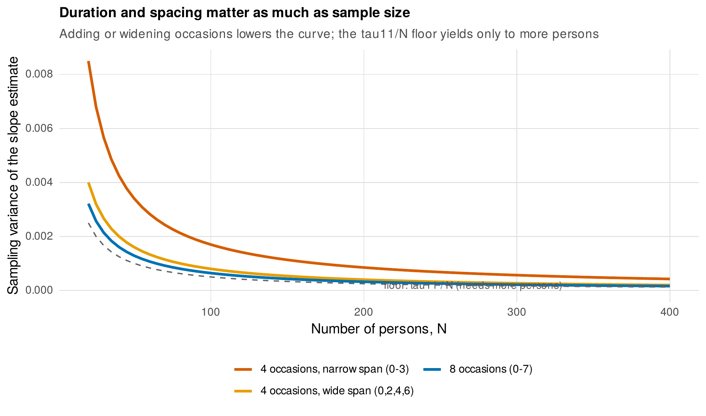
Note. Analytic sampling variance of the average slope (Equation 4.2) against the number of persons, for three occasion designs. Adding or widening occasions lowers the curve; the dashed line is the \(\tau_{11}/N\) floor, reducible only by adding persons. Parameters are illustrative (\(\tau_{11}=0.05\), \(\sigma^2=0.6\)).
Beyond these cases the formulas become fragile. Generalized linear mixed models, latent growth models with many parameters, and intensive longitudinal models with autoregressive structure rarely admit trustworthy closed-form power, because the standard error of a target parameter depends on the entire model in ways no simple formula captures. For these, the honest and general tool is simulation, and learning it well makes the closed forms optional conveniences rather than necessities.
4.3 The Simulation-Based Power Workflow
Simulation-based power analysis is a single reusable skill: specify the process that generates the data, generate many datasets from it, fit the analysis model to each, and count how often the target effect is detected. The proportion detected is the power. The workflow has six steps, shown in Figure 4.3, and the same skeleton powers any model by swapping the data-generating function and the analysis.
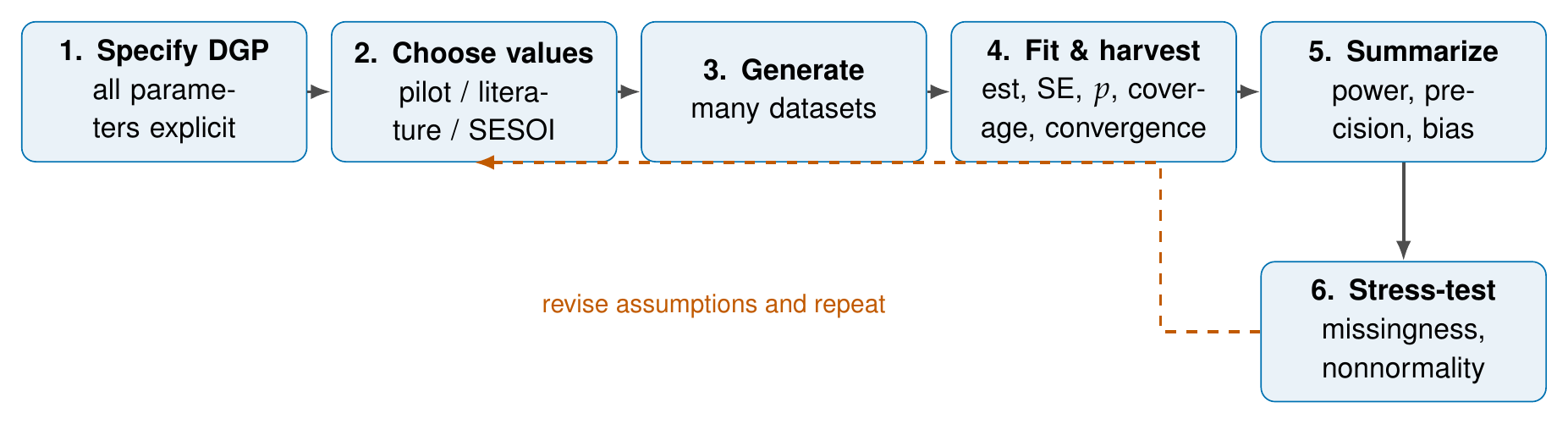
Note. The same skeleton applies to any model: only the data-generating process (Step 1) and the analysis (Step 4) change. Step 6 feeds back into Step 2, because a power analysis is a sensitivity analysis over uncertain assumptions, not a single calculation.
The code below is the complete engine, applied to a daily-diary model in which a within-person predictor and a person-level moderator jointly affect an outcome. It is deliberately compact; the companion power_sim_template.R is the same logic with comments, and later chapters reuse it.
library(lme4)

# STEP 1: the data-generating process, every parameter explicit
sim_diary <- function(N, D, g10 = 0.15, g01 = 0.20, g11 = 0.10,
                      tau00 = 0.25, tau11 = 0.03, sigma = sqrt(0.5)) {
  person <- rep(seq_len(N), each = D)
  w <- rep(rnorm(N), each = D); x <- rnorm(N * D)          # moderator, predictor
  u0 <- rep(rnorm(N, 0, sqrt(tau00)), each = D)            # random intercept
  u1 <- rep(rnorm(N, 0, sqrt(tau11)), each = D)            # random slope
  y  <- u0 + (g10 + u1)*x + g01*w + g11*x*w + rnorm(N*D, 0, sigma)
  data.frame(person, x, w, y)
}

# STEPS 3-4: generate, fit, harvest one replication's results
one_rep <- function(N, D) {
  d <- sim_diary(N, D)
  f <- lmer(y ~ x + w + x:w + (1 + x | person), data = d)
  b <- fixef(f); s <- sqrt(diag(vcov(f)))
  data.frame(p_within = 2*pnorm(-abs(b["x"]/s["x"])),      # within-person effect
             converged = length(f@optinfo$conv$lme4$messages) == 0)
}

# STEP 5: summarize power over many replications (STEP 2 = the chosen values)
set.seed(2026)
reps <- do.call(rbind, replicate(500, one_rep(N = 40, D = 14), simplify = FALSE))
reps <- reps[reps$converged, ]                             # convergence bookkeeping
mean(reps$p_within < 0.05)                                 # estimated power ~ 0.95
Three features of this workflow separate a trustworthy power analysis from a misleading one. The first is convergence bookkeeping. Mixed models fail to converge on some simulated datasets, especially at small samples, and silently dropping those datasets inflates the reported power, because the failures are not random with respect to the effect. The honest practice is to record the convergence status of every fit, report the convergence rate, and decide in advance how non-converged fits count; treating them as non-detections is conservative and defensible. The second is seed management: a single seed at the top makes the entire analysis reproducible, and for parallel execution a parallel-safe generator (such as L’Ecuyer streams) is required so that workers do not share or repeat random numbers. The third is that the parameter values in Step 2 are where power analyses live or die.
Common Pitfall • three ways a power analysis goes wrong
First, observed (post hoc) power: computing power from the effect size actually observed in a completed study is uninformative, because observed power is a monotone function of the \(p\) value and adds nothing to it; a nonsignificant result always has low observed power by construction. Power analysis is a design activity, done before data collection. Second, powering only the fixed main effect: reporting that a study has \(.90\) power for the average slope, while the actual scientific claim concerns individual differences in slopes or a cross-level interaction, advertises power for the easy estimand and hides the hard one (Figure 4.1). Power the estimand that carries the claim. Third, ignoring convergence failures: summarizing power only over the datasets that converged, without reporting how many did not, biases the estimate upward and conceals a design that is too ambitious for its sample.
Where do the parameter values come from? This is the “garbage in, garbage out” problem of power analysis, and it has no fully satisfying solution, only disciplined options summarized in Table 4.1. Pilot data give realistic variance components but, when small, give noisy and often inflated effect estimates. The published literature supplies effect sizes but is distorted by publication bias, so that planning to the published effect plans to an inflated target and yields an underpowered study. The most defensible anchor is often the smallest effect size of interest, the effect below which the finding would not matter substantively, because powering for it guarantees the study can detect anything worth detecting (Lakens, 2022). Whatever the source, the remedy for uncertainty in the inputs is to report power across a plausible range of parameter values, a sensitivity curve rather than a single number, so that the reader sees how the conclusion depends on assumptions.
Table 4.1. Where the parameters for a power analysis come from.
| Source | What it provides | Caution |
|---|---|---|
| Pilot data | Realistic variance components and correlations | Small pilots give noisy, upwardly biased effect sizes |
| Published literature | Plausible effect sizes | Publication bias inflates effects (the winner’s curse) |
| Smallest effect of interest (SESOI) | A principled lower bound to power for | Requires an explicit substantive judgment |
| Sensitivity analysis | Power across a range of plausible values | Report the curve, not a single convenient number |
Note. Combining sources is common: variance components from a pilot, an effect at the SESOI, and a sensitivity sweep over the least certain inputs.
4.4 Tool Shortcuts for Standard Cases
Writing the simulation from scratch is the general skill, but for standard models existing tools remove the boilerplate. Table 4.2 maps common model families to tools. For lme4 models, simr wraps the whole workflow: it simulates from a fitted or specified model and reports power and power curves over sample size (Green & MacLeod, 2016). For two- and three-level trial designs, powerlmm offered convenient closed-form and simulation power, though its package status should be verified at the time of writing and equivalent custom code substituted if it is unavailable. For latent growth and structural models, lavaan’s data-simulation facility paired with a fitting loop implements the same Monte Carlo logic, and Mplus’s MONTECARLO routine is the field’s long-standing workhorse for latent-variable power (Muthén & Muthén, 2002; Muthén & Curran, 1997). For intensive longitudinal designs with autoregressive structure, the Shiny application of Lafit and colleagues (2021) performs power analysis for multilevel models that respect temporal dependence, which off-the-shelf tools ignore. Whatever the tool, the same three disciplines apply: name the estimand, source the parameters honestly, and report sensitivity.
Table 4.2. Tools for longitudinal power analysis.
| Tool | Model family | Strengths | Limits |
|---|---|---|---|
| simr | lme4 LMM/GLMM | Wraps simulate-fit-count; power curves | Slow on large grids; lme4 only |
| powerlmm | 2–3 level trials | Fast for standard trial designs | Verify CRAN status; limited classes |
| lavaan Monte Carlo | LGM / SEM | Flexible; you control the loop | Requires custom code |
Mplus MONTECARLO | LGM / GMM / DSEM | Field standard for latent power | Licensed software |
| Lafit et al. Shiny app | Multilevel AR (ILD) | Respects temporal dependence | Fixed model menu |
| Custom simulation | Any | Full control; the general skill | You must write and validate it |
Note. Package availability changes; verify at write-up. A custom simulation is always available as the fallback and is the skill the others automate.
4.5 Three Worked Power Analyses
The three design vignettes of Chapter 2 return here as power analyses, each producing a figure and a grant-ready paragraph.
4.5.1 The daily-diary study: cheap main effects, expensive interactions
The stress-and-sleep diary asks two questions: whether daily stress predicts that night’s sleep within persons, and whether that within-person coupling is moderated by a person-level trait. The first is a within-person main effect; the second is a cross-level interaction. Figure 4.4 shows the power for the within-person effect across a grid of persons and days: it is cheap, exceeding \(.80\) by forty persons measured for a week and saturating quickly thereafter, because within-person effects draw on the many occasions each person contributes. Figure 4.5 contrasts that main effect with the cross-level interaction on the same axis. The interaction is expensive: at fourteen days it reaches \(.80\) power only near seventy persons, roughly double the sample the main effect needs, because a cross-level interaction is estimated essentially at the between-person level, where the unit of information is the person, not the occasion. This is the single most important planning lesson for diary and experience-sampling studies, and it is routinely missed: adding days does little for a cross-level interaction, whereas adding persons is decisive.
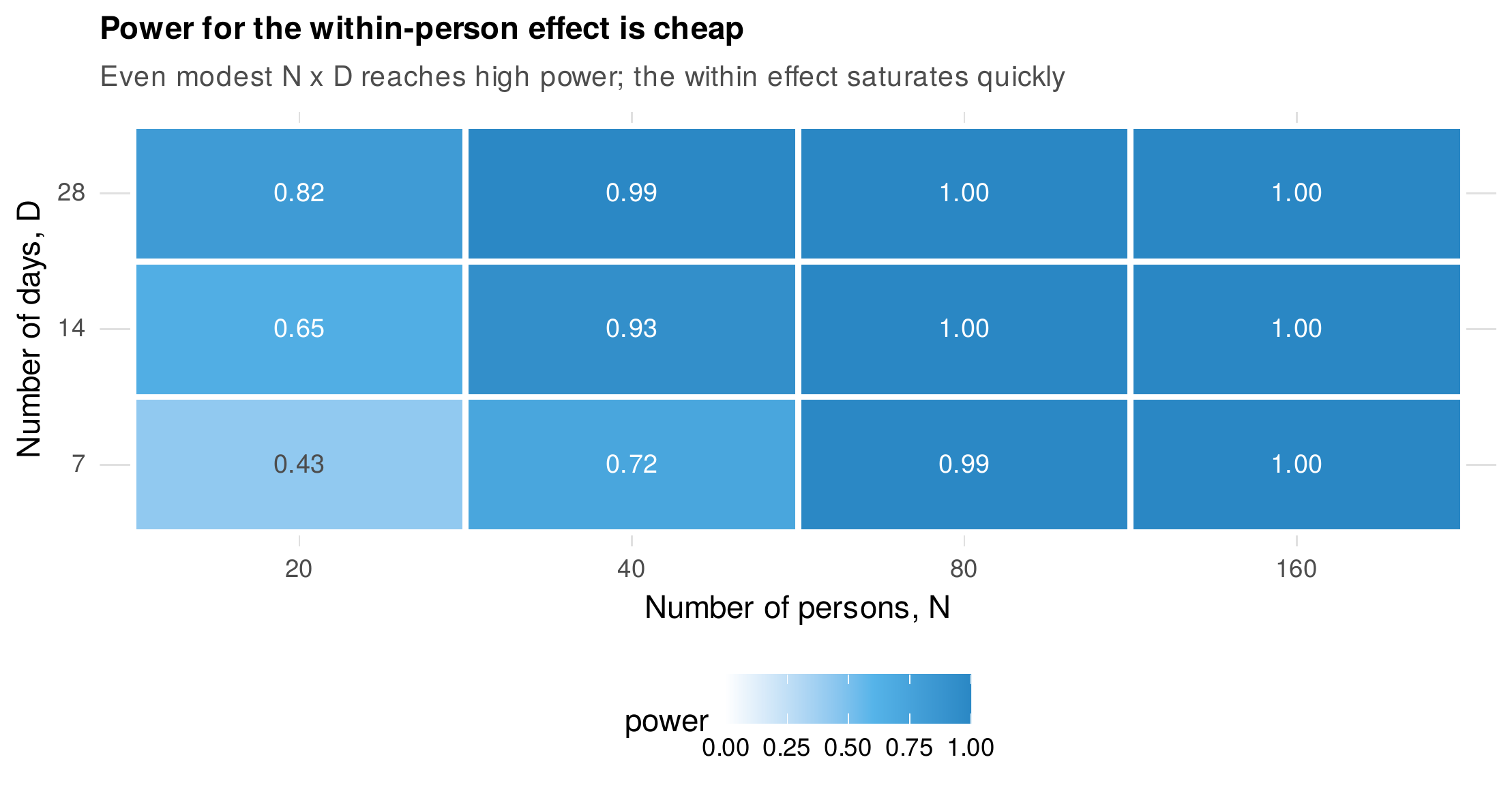
Note. Simulated power (each cell \(300\) replications) for the within-person effect of a daily predictor, as a function of the number of persons and days. The within-person effect reaches high power at modest sample sizes and saturates.
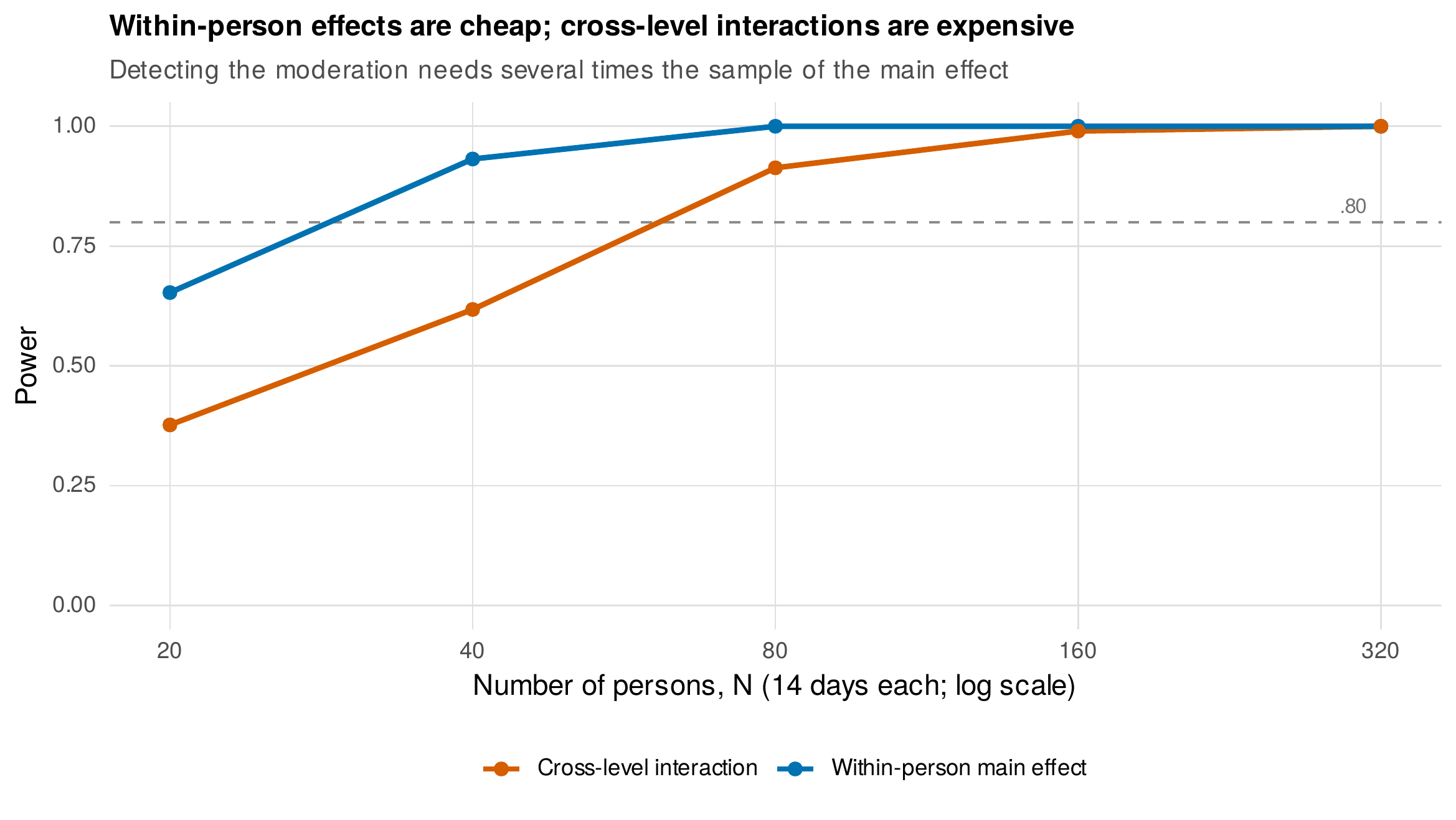
Note. Simulated power at fourteen days per person. The within-person main effect (blue) reaches \(.80\) near thirty persons; the cross-level interaction (red) requires roughly twice as many, and adding days would not close the gap.
A grant-ready paragraph for this study reads: “The primary hypothesis concerns the cross-level interaction between daily stress and trait rumination in predicting sleep. Assuming a within-person stress-sleep slope of \(0.15\), a moderation of \(0.10\), random-slope variance of \(0.03\), and residual variance of \(0.50\) (from pilot data and the smallest effect of interest), a Monte Carlo power analysis of \(300\) replications per condition indicates that \(120\) participants completing a fourteen-day diary provide power of at least \(.90\) to detect the interaction at \(\alpha = .05\). Sensitivity analyses over moderation values from \(0.07\) to \(0.13\) yield power from \(.72\) to \(.98\); convergence exceeded \(99\%\) across conditions.”
4.5.2 The accelerated growth study: detecting individual differences in change
The accelerated-cohort achievement study (the school_growth design) asks not only whether children grow but whether they differ in how fast they grow, that is, whether the random slope variance is nonzero. As Equation (4.2) foretold, this is a large-\(N\) question. Figure 4.6 shows power for the slope variance rising from about \(.45\) at fifty children to essentially one at four hundred, crossing \(.80\) near one hundred fifty. A study sized to estimate the average growth trajectory, which needs far fewer children, would be badly underpowered for the individual-differences question that often motivates developmental research (Hertzog, Lindenberger, Ghisletta, & von Oertzen, 2006). Naming which of the two questions is primary is the first act of planning such a study.
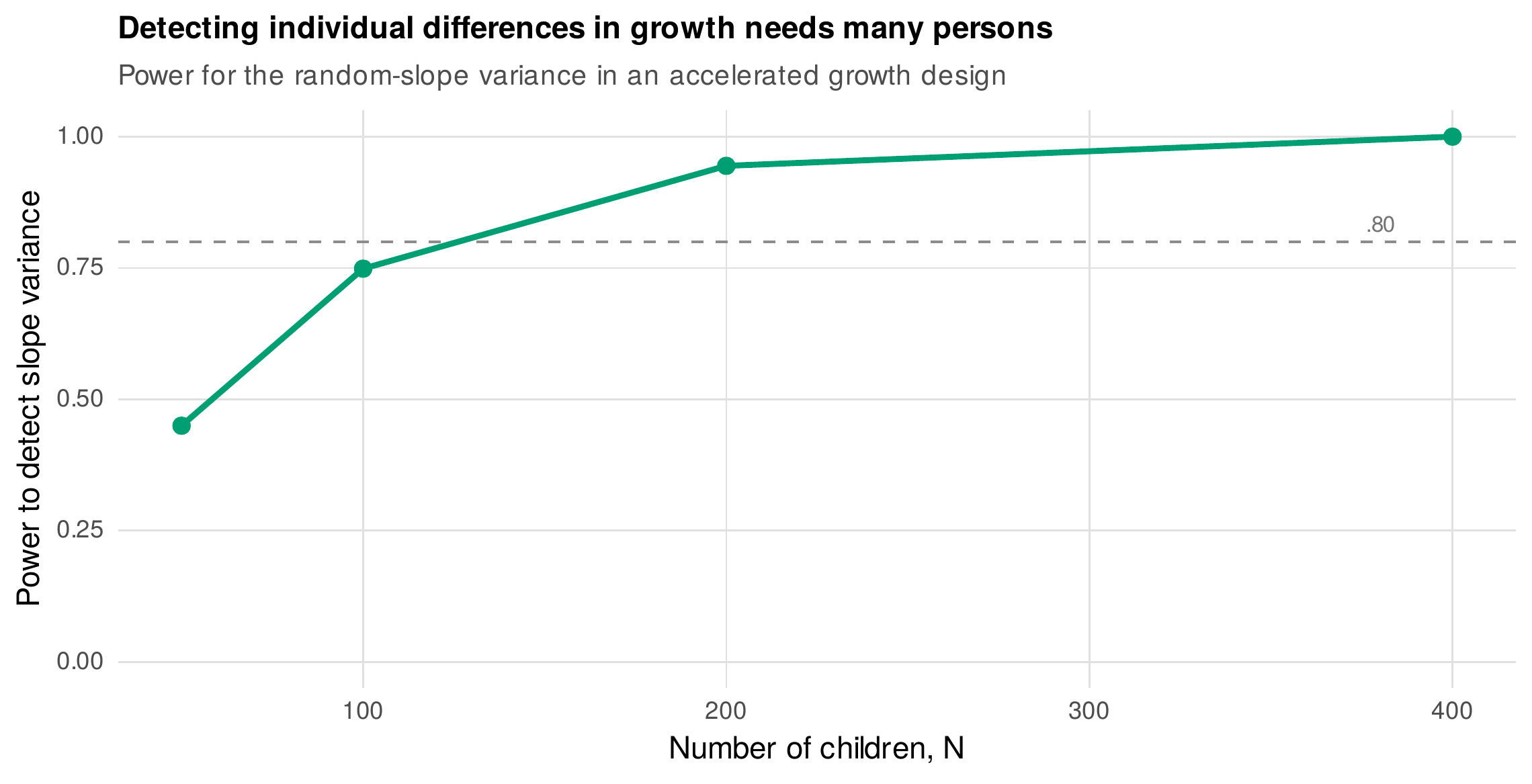
Note. Simulated power (\(200\) replications per point) for the likelihood-ratio test of random-slope variance in a four-wave growth model, as a function of the number of children. Detecting variance in change requires many persons, consistent with Equation (4.2).
4.5.3 The clinical trial: powering under realistic dropout
The two-arm depression trial (the therapy_rct design) tests a treatment-by-time interaction: whether the treatment arm’s symptom trajectory declines faster than the control arm’s. Trials lose participants, and a planner must ask what dropout does to power. Figure 4.7 shows power for the interaction across sample sizes under zero, fifteen, and thirty percent missing-at-random dropout. The instructive result is that the loss is gentle: at eighty patients, power falls from about \(.68\) under no dropout to about \(.55\) under thirty percent dropout, a real but modest reduction. The reason matters and anticipates Chapter 6. Because the mixed model estimates the trajectory by likelihood, using every observation each patient did provide, missing-at-random dropout costs information and hence power, but does not bias the estimate. The naive alternative of analyzing only completers would both lose more power and, because completers differ systematically from dropouts, introduce bias. Planning for dropout therefore means inflating the sample modestly to offset the precision loss, not treating dropout as a catastrophe, provided the missingness is plausibly at random and the analysis is likelihood-based.
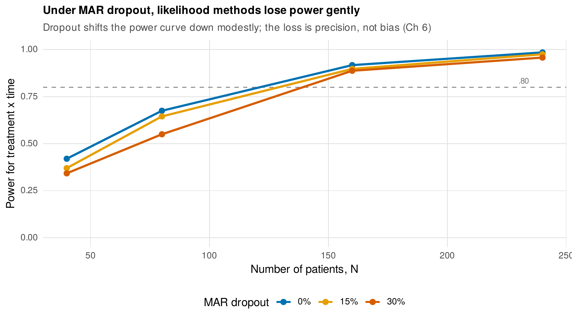
Note. Simulated power (\(400\) replications per point) for the treatment-by-time interaction in a twelve-week trial, under three levels of monotone missing-at-random dropout. Dropout shifts the curve down modestly; the cost is precision, not bias, because the likelihood uses all available data (Chapter 6).
4.6 Designing Under Constraints
Power analysis meets reality as a budget. Persons, occasions, and per-occasion density each cost money and participant goodwill, and they buy power for different estimands, as Table 4.3 summarizes. The central trade-off is between the number of persons and the number of occasions. For a fixed number of total observations, the split is not neutral: between-person estimands and cross-level interactions are bought by persons, whereas within-person effects, growth shape, and dynamics are bought by occasions. A study of one hundred persons measured ten times and a study of ten persons measured one hundred times contain the same thousand observations and answer almost disjoint questions, which is why the folklore that “it is the total \(N \times T\) that matters” is false. The design must be matched to the estimand, and the budget spent where the estimand’s information lives.
Table 4.3. Which design factor buys power for which estimand.
| Increasing... | Mainly buys power for | Does little for |
|---|---|---|
| Persons (\(N\)) | Between-person effects, cross-level interactions, all variance components | (raises precision for all) |
| Occasions (\(T\)) | Within-person effects, growth shape, dynamics | Between-person mean differences |
| Duration / spacing | Growth-slope precision, slope variance | Fast dynamics (risk of aliasing) |
| Items per occasion | All effects, via higher reliability (less attenuation) | Design-level power directly |
Note. The table operationalizes Equation (4.2) and its analogues: match the budget to where the estimand’s information lives.
Precision planning offers a second lens on the same budget. Figure 4.8 shows the expected width of the confidence interval for the within-person effect as a function of the number of persons: to pin the effect down to a width of \(0.10\) requires about one hundred persons, regardless of whether that sample would clear a power threshold. When a reviewer insists on \(.80\) power for a variance component that no feasible sample could reach, the precision framing supplies an honest response, reporting the interval width the study will achieve and arguing that a well-estimated bound is more informative than an underpowered test. Two further tools stretch a fixed budget. Planned missingness designs, in which each participant is deliberately assigned only a subset of items or occasions, can preserve power for the primary estimand at reduced burden (Chapter 6). And sequential or internal-pilot designs allow variance components to be re-estimated partway through, refining the sample-size decision with accumulating data. Table 4.4 distills the reporting into a template.
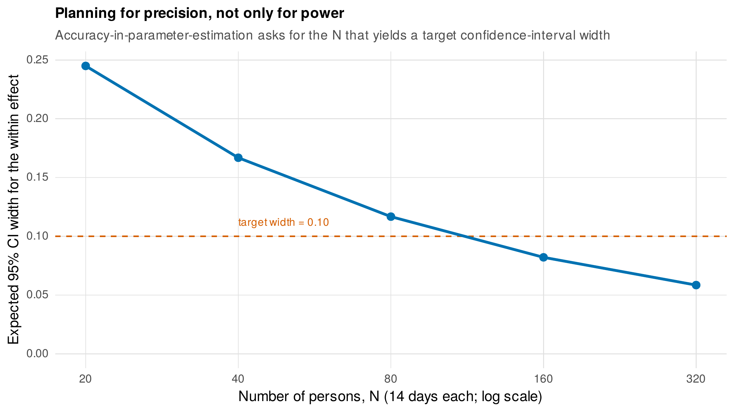
Note. Simulated expected width of the \(95\%\) confidence interval for the within-person effect at fourteen days per person. The accuracy-in-parameter-estimation question is the sample size that achieves a target width (here \(0.10\), near one hundred persons), complementing the power question of Figure 4.4.
Table 4.4. Elements of a defensible sample-size justification.
| Element | What to state |
|---|---|
| Estimand | The target quantity, in words, and why it carries the claim |
| Analysis model | The model to be fitted, so the reader can judge the estimand’s standard error |
| Parameters and source | The assumed values and where each came from (pilot, literature, SESOI) |
| Power or precision | The power at the planned \(N\), or the confidence-interval width, with the method and number of replications |
| Sensitivity | Power or precision across a plausible range of the least certain inputs |
| Contingency | The assumed dropout and compliance, and how the sample is inflated to offset them |
Note. These elements make a power analysis auditable and are increasingly expected in preregistrations and grant applications (Chapter 36).
In Practice • runtime and checkpointing for large power grids
A power analysis over a grid of conditions can require tens of thousands of model fits, and the runtime is easy to underestimate. Time a single fit, multiply by replications and grid cells, and divide by the number of cores before launching; a grid that runs overnight is normal, one that runs for a week needs rethinking. Parallelize across replications with a parallel-safe random-number generator so results remain reproducible. For long runs, save results condition by condition to disk (checkpointing), so that an interrupted run resumes rather than restarts, and so that partial results can be inspected. Begin development with a small number of replications to debug the pipeline, and raise it only once the workflow is correct; a power estimate from twenty-five replications is useless for a final answer but perfect for confirming the code runs.
Software Note • Mplus Monte Carlo for latent growth models
For latent growth and mixture models, Mplus’s MONTECARLO facility remains the field standard. The logic mirrors the R workflow of Section 4.3: a MODEL POPULATION block specifies the data-generating parameters, a MODEL block specifies the analysis, and Mplus repeatedly generates and fits, returning the proportion of replications in which each parameter is significant (power) together with parameter bias, standard-error accuracy, and coverage. The approach was codified by Muthén and Muthén (2002) and is the natural tool when the analysis model is itself a structural equation model, where writing the generation and fitting by hand in R is more laborious. The reporting discipline is identical: name the estimand, justify the population values, and present sensitivity.
4.7 Common Misconceptions
Four beliefs mislead planners. First, that what matters is the total number of observations \(N \times T\): information is level-specific, so ten persons measured one hundred times cannot answer the between-person questions that one hundred persons measured ten times can, despite equal totals. Second, that attrition only reduces power: under missing-at-random dropout and a likelihood-based analysis the cost is indeed mainly power (Figure 4.7), but under missing-not-at-random dropout it also biases estimates, which no sample size fixes (Chapter 6). Third, that a power analysis is one number: it is a curve or surface over design factors, plus the assumptions that generated it, and reporting a lone number hides both. Fourth, the practical predicament, “reviewers demand \(.80\) power for everything, but my slope-variance power is \(.40\)”: the answer is not to inflate assumptions until the number looks acceptable, but to state honestly which estimands are well powered and which are estimated for precision, and to justify the design in those terms (Lakens, 2022).
Chapter Summary
Power in longitudinal models is estimand-specific: the same study is generously powered for some quantities and helpless for others (Figure 4.1), so planning begins by naming the estimand that carries the scientific claim. Closed-form results survive only for simple designs, but they yield one durable insight, that the slope-estimator variance (Equation 4.2) splits into a term reducible by occasions and spacing and a \(\tau_{11}/N\) floor reducible only by persons. For realistic models the general tool is the six-step simulation workflow, whose integrity rests on convergence bookkeeping, reproducible seeds, and honest parameter sourcing anchored on the smallest effect of interest. The three worked analyses teach the recurring lessons: within-person effects are cheap and cross-level interactions expensive, detecting individual differences in change is a large-\(N\) enterprise, and missing-at-random dropout costs precision rather than bias. Planning is finally a budget problem, solved by matching persons, occasions, and density to where the estimand’s information lives, and reported in estimand-first, precision-aware language.
Where to Go Next
The stress tests of this chapter’s simulations use the missingness mechanisms formalized in Chapter 6, and the models treated here as black boxes are developed in Chapters 13 and 14 (multilevel growth), 19 (latent growth), and 23 (intensive longitudinal). Bayesian planning, which replaces a single power number with an assurance averaged over prior uncertainty, appears in Chapter 17. The power analysis is itself a preregisterable object, and Chapter 36 treats its preregistration. The reusable power_sim_template.R introduced here recurs in the exercises of later chapters, where the DGP is swapped for each new model.
Exercises
- 4.1 Add nonresponse. Extend the diary power simulation of Section 4.3 to delete \(20\%\) of person-occasions completely at random before fitting. Report the change in power for the within-person effect and explain it in terms of lost information.
- 4.2 Use simr. Take a small pilot dataset (for example
sleepstudy), fit a random-slope model, and use simr to compute a power curve over sample size for the fixed slope. Compare the result with a from-scratch simulation. - 4.3 Precision (AIPE). Using the diary DGP, find by simulation the number of persons needed so that the \(95\%\) confidence interval for the standardized within-person effect has width no greater than \(0.10\). Contrast this \(N\) with the \(N\) that yields \(.80\) power.
- 4.4 Critique a power statement. Given a published sample-size justification, identify which estimand was powered, which assumptions were stated, and what a skeptical reviewer would still want to know.
- 4.5 Write the justification. Using Table 4.4, write the sample-size paragraph for the accelerated growth study of Section 4.5, powering the slope-variance estimand and including a sensitivity analysis.
References
Arend, M. G., & Schäfer, T. (2019). Statistical power in two-level models: A tutorial based on Monte Carlo simulation. Psychological Methods, 24(1), 1–19. https://doi.org/10.1037/met0000195
Bolger, N., Stadler, G., & Laurenceau, J.-P. (2012). Power analysis for intensive longitudinal studies. In M. R. Mehl & T. S. Conner (Eds.), Handbook of research methods for studying daily life (pp. 285–301). Guilford Press.
Cohen, J. (1988). Statistical power analysis for the behavioral sciences (2nd ed.). Lawrence Erlbaum Associates.
Green, P., & MacLeod, C. J. (2016). SIMR: An R package for power analysis of generalized linear mixed models by simulation. Methods in Ecology and Evolution, 7(4), 493–498. https://doi.org/10.1111/2041-210X.12504
Hertzog, C., Lindenberger, U., Ghisletta, P., & von Oertzen, T. (2006). On the power of multivariate latent growth curve models to detect correlated change. Psychological Methods, 11(3), 244–252. https://doi.org/10.1037/1082-989X.11.3.244
Lafit, G., Adolf, J. K., Dejonckheere, E., Myin-Germeys, I., Viechtbauer, W., & Ceulemans, E. (2021). Selection of the number of participants in intensive longitudinal studies: A user-friendly Shiny app and tutorial for performing power analysis in multilevel regression models that account for temporal dependencies. Advances in Methods and Practices in Psychological Science, 4(1). https://doi.org/10.1177/2515245920978738
Lakens, D. (2022). Sample size justification. Collabra: Psychology, 8(1), 33267. https://doi.org/10.1525/collabra.33267
Maxwell, S. E., Kelley, K., & Rausch, J. R. (2008). Sample size planning for statistical power and accuracy in parameter estimation. Annual Review of Psychology, 59, 537–563. https://doi.org/10.1146/annurev.psych.59.103006.093735
Muthén, B. O., & Curran, P. J. (1997). General longitudinal modeling of individual differences in experimental designs: A latent variable framework for analysis and power estimation. Psychological Methods, 2(4), 371–402. https://doi.org/10.1037/1082-989X.2.4.371
Muthén, L. K., & Muthén, B. O. (2002). How to use a Monte Carlo study to decide on sample size and determine power. Structural Equation Modeling, 9(4), 599–620. https://doi.org/10.1207/S15328007SEM0904_8
Raudenbush, S. W., & Liu, X. (2000). Statistical power and optimal design for multisite randomized trials. Psychological Methods, 5(2), 199–213. https://doi.org/10.1037/1082-989X.5.2.199
Raudenbush, S. W., & Liu, X.-F. (2001). Effects of study duration, frequency of observation, and sample size on power in studies of group differences in polynomial change. Psychological Methods, 6(4), 387–401. https://doi.org/10.1037/1082-989X.6.4.387
Snijders, T. A. B., & Bosker, R. J. (2012). Multilevel analysis: An introduction to basic and advanced multilevel modeling (2nd ed.). Sage.