Chapter 5
Preparing and Managing Repeated Measures Data
This is the chapter that will save you the most time and the fewest citations. Between a raw data export and a fitted model lies a stretch of unglamorous work, reshaping, aligning time, merging, screening, deriving, that is usually invisible in published papers and yet routinely moves the results. The decisions made here are not pre-scientific housekeeping; they are analytic choices, and they deserve the same documentation and defense as a model specification.
Learning Objectives
After working through this chapter, you should be able to: (1) convert between wide and long formats and say which models require which; (2) construct principled time variables, wave, study day, clock time, event time, and age, and defend the choice against the research question; (3) merge multi-wave and multi-source data with disciplined key hygiene and join validation; (4) compute compliance metrics and produce a compliance report; (5) detect careless or invalid intensive responses from response times and invariant response strings; (6) construct within-person lags correctly, including the night-gap decision; and (7) package a dataset with a codebook for archiving.
5.1 Shapes of Repeated Measures Data
Repeated measures data live in two canonical shapes and one informal one. In wide format each person occupies a single row and the repeated measurements spread across columns, one per occasion. In long format each person contributes one row per occasion, so that a single outcome column is indexed by a person identifier and a time variable. The informal third shape, a list of streams, arises in intensive and multi-source studies where self-report, physiology, and passive sensing arrive as separate files sampled on different clocks, to be aligned later. Figure 5.1 shows the same three persons in wide and long form. The canonical analysis-ready structure for this book is long, with one row per person-occasion, because it is what multilevel and most modern software expects; Table 5.1 states which model families require which shape.
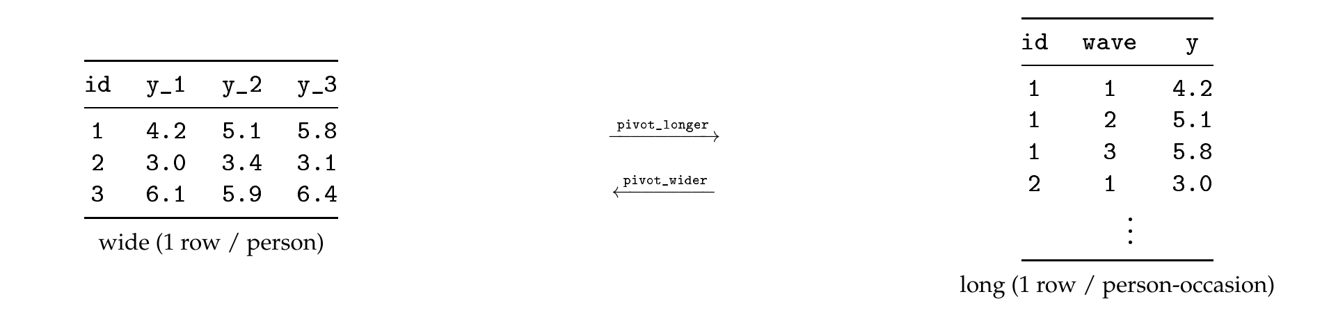
Note. Wide format stores one row per person with occasions in columns; long format stores one row per person-occasion. The tidyverse verbs pivot_longer and pivot_wider convert between them.
The conversion is one line each way. The essential idioms, which cover most longitudinal reshaping, name the occasion variable explicitly and strip any prefix from the column names so that the time index is clean.
library(tidyverse)
# wide -> long: one row per person-occasion (for MLM, GEE, plotting)
long <- wide %>%
  pivot_longer(cols = starts_with("y_"), names_to = "wave",
               names_prefix = "y_", values_to = "y") %>%
  mutate(wave = as.integer(wave))

# long -> wide: (for RM-ANOVA, and the wide convention of some SEM setups)
wide <- long %>%
  pivot_wider(names_from = wave, values_from = y, names_prefix = "y_")
When several scales are measured at each occasion, the wide column names encode two facts at once, the variable and the wave, and pivot_longer can split them with a names_pattern, for example turning na_w1, pa_w1, na_w2, ... into a long table with separate na and pa columns indexed by wave. Throughout the book the house conventions are snake_case variable names, a stable integer or string person identifier named id or person, and a var_wave suffix for wide columns, so that reshaping is mechanical rather than improvised.
Table 5.1. Which data shape each model family expects.
| Model family | Shape | Note |
|---|---|---|
| Repeated-measures ANOVA / MANOVA | Wide | One row per person; occasions as columns |
| Multilevel / mixed models (Ch. 13, 23) | Long | One row per person-occasion |
| Generalized estimating equations (Ch. 12) | Long | Long with a person cluster id |
| Structural equation / latent growth (Ch. 19) | Wide\(^{a}\) | Classic SEM uses wide; some software now accepts long |
| Plotting (ggplot2) | Long | The grammar of graphics maps long columns to aesthetics |
Note. \(^{a}\)Latent growth models in lavaan conventionally read wide data (one column per occasion). Keep a long master file and pivot to wide when needed, not the reverse.
5.2 Time Is a Variable You Build
The time index is not given by the data; it is constructed, and the construction is a modeling decision disguised as data cleaning. The same observations can be indexed by at least five different clocks, and each answers a different question. Wave counts assessments as equal integers, convenient but silent about real spacing. Clock time records the calendar date and time of day. Study time counts days since enrollment. Event time counts time relative to a meaningful event, a quit attempt, a diagnosis, a bereavement. Developmental time is age. Figure 5.2 plots one person’s craving ratings across a smoking-cessation study under five clocks. Against wave the sharp drop looks gradual; against clock time it is meaningless noise; against study day and, most clearly, against time-to-quit, the drop aligns with the event that caused it. Choosing the clock that matches the process is the difference between seeing the phenomenon and hiding it, and the choice recurs as a central decision in the growth models of Chapter 14. Table 5.2 is a construction guide.
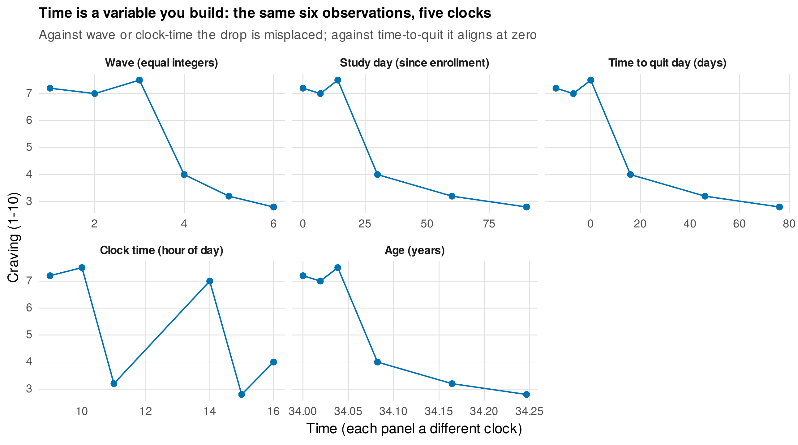
Note. One person’s craving ratings in a cessation study, plotted against wave, study day, time-to-quit, clock time, and age. The clock chosen determines whether the change aligns with its cause. Keep every clock in the data; discard none at cleaning time.
Intensive designs add their own timekeeping hazards. A beep number is not a timestamp: two people’s third beep of the day occur at different moments, and the response may arrive minutes after the prompt, so both the scheduled time and the actual response time must be recorded, and the latency between them retained as data (it will screen careless responses below and, in Chapter 27, feed continuous-time models). Defining a “day” requires a decision for populations who are awake past midnight; a three-in-the-morning cutoff often groups a late-night response with the correct day. And time zones and daylight saving are not pedantry but genuine bugs: a study spanning a clock change, or a device exporting in a different zone, will silently misorder observations unless timestamps are parsed with zone awareness. The discipline is to parse every timestamp with an explicit zone using lubridate, and to convert everything to a single study clock before ordering.
library(lubridate)
# Parse zone-aware; the device-swap participant's rows were exported in UTC.
resp <- ymd_hms(raw$response_ts, tz = "Asia/Seoul")
utc  <- raw$tz == "UTC"
resp[utc] <- with_tz(force_tz(resp[utc], "UTC"), "Asia/Seoul")  # to study clock
raw$latency_sec <- as.numeric(resp - ymd_hms(raw$scheduled_ts, tz = "Asia/Seoul"))
Table 5.2. Constructing time variables: five clocks and the questions they serve.
| Clock | Definition | Question it serves |
|---|---|---|
| Wave | Assessment number (1, 2, 3, …) | Occasion effects when spacing is equal or irrelevant |
| Study time | Days since enrollment | Change indexed to the study protocol |
| Clock / calendar time | Date and time of day | Diurnal and day-of-week effects; ordering |
| Event time | Time since or until an event | Change organized by a cause (quit day, onset) |
| Developmental time | Age | Growth and aging over the life span |
Note. Build and keep several clocks in the analysis file. Record the exact response timestamp (time_actual) even when the analysis uses waves, because later continuous-time models (Chapter 27) require the real intervals.
5.3 Merging and Validating
Joining longitudinal data is where silent errors enter, because a mismatched key does not raise an error; it simply drops or duplicates rows. The discipline is to audit before merging. An anti_join between two tables returns exactly the rows in the first with no match in the second, so running it first reveals orphaned records before a left_join quietly discards them, and a count of keys reveals duplicates before they multiply rows. Figure 5.3 shows the loop. Multi-wave studies compound the difficulty because variable names drift across waves, the achievement column called ach in wave one becomes score in wave four, so the rename mapping should be held as data, a small table of old and new names, rather than scattered through the code where it cannot be checked.

Note. An anti_join run before the left_join surfaces keys that would otherwise be silently dropped. Merges keep every participant (attrition is handled at analysis, Chapter 6), so a left_join from the wave data preserves all records.
# A rename map held as data, applied per wave, then audited before merging.
orphans <- anti_join(waves, roster, by = "child_id")   # audit BEFORE the join
stopifnot(nrow(orphans) == 0)                           # fail loudly, not silently
dup_keys <- waves %>% count(child_id, wave) %>% filter(n > 1)
stopifnot(nrow(dup_keys) == 0)
long <- left_join(waves, roster, by = "child_id")       # keep every child
Multi-source alignment, joining self-report to actigraphy or physiology, adds the problem that streams are sampled on different clocks and rarely at the same instants. The tools are nearest-timestamp joins with an explicit tolerance window (match each self-report to the sensor reading within, say, five minutes), and deliberate resampling or aggregation decisions, each documented as a decision rather than performed silently. The rule throughout is that any operation that could drop or duplicate a row is preceded by an audit that would fail loudly if it did.
5.4 Screening Intensive Data
Intensive data must be screened for two distinct problems: whether prompts were answered, and whether the answers can be trusted. Compliance is the ratio of completed to scheduled prompts, and the cardinal rule is to look at it before summarizing it, because a single percentage hides the pattern that matters. Figure 5.4 shows a compliance heatmap for the book’s experience-sampling study: each cell is one person-day, shaded by the number of valid responses, with persons ordered by total compliance. The display reveals what a mean cannot, that low compliance is concentrated in particular people and drifts downward over the study, a pattern with direct consequences for missing-data modeling (Chapter 6). For the study shown, overall compliance was \(72.8\%\), with a median per-person compliance of \(73\%\) and a range from \(58\%\) to \(85\%\).
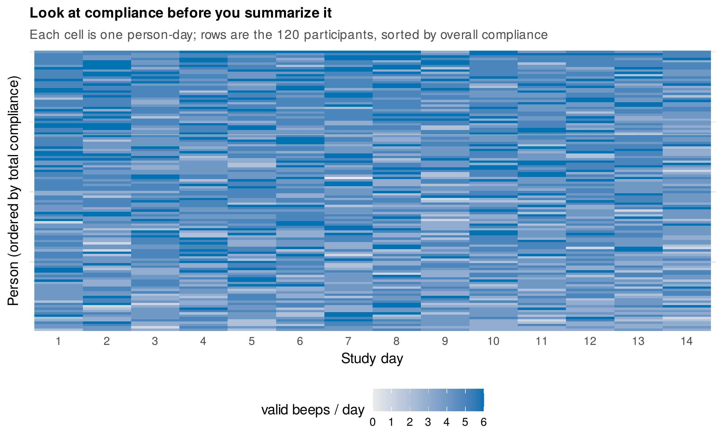
Note. Each cell is one person-day in the affect_ema study, shaded by the number of valid responses (of six scheduled). Rows are the 120 participants, ordered by total compliance. Patterning, not the overall percentage, is what threatens inference.
Whether answers can be trusted is the problem of careless responding, and intensive designs, with their many low-stakes prompts, are especially prone to it. Three signatures are detectable without any special package. Ultra-fast completions, a response submitted in under a few seconds, cannot reflect genuine reflection. Invariant response strings, the same value chosen for every item on a prompt, indicate straight-lining; the longstring index, the longest run of identical consecutive item responses, captures this, and a run spanning items of opposite valence (negative- and positive-affect items alike) is a strong signal. Impossible sequences and out-of-range values round out the screen. Figure 5.5 shows the screening dashboard for the same study: a response-time distribution with the too-fast and out-of-window regions marked, and the longstring distribution with the straight-lining cases flagged. Applying these screens flagged \(45\) out-of-window responses and \(26\) careless responses in a raw export of \(7{,}374\) rows.
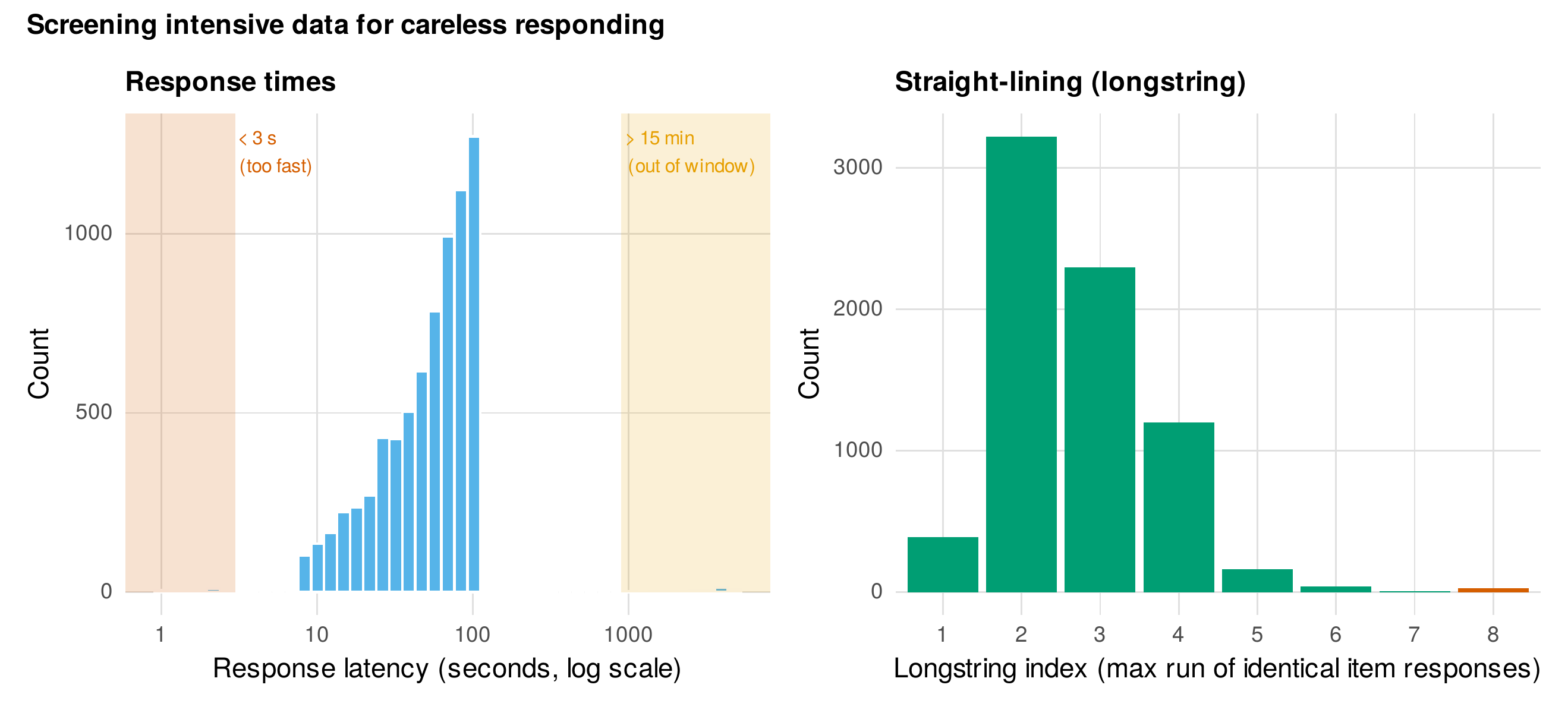
Note. Left: the distribution of response latencies (log scale), with the under-three-second (too fast) and over-fifteen-minute (out of window) regions marked. Right: the distribution of the longstring index, with straight-lining responses (a run of eight identical answers) flagged in red.
The cardinal principle of screening is to flag, not drop. Every screen adds a Boolean column to the data rather than deleting a row, so that the analysis script, not the cleaning script, decides what to exclude, and so that a sensitivity analysis with and without flagged cases is a one-line change. Exclusion rules should be preregistered where possible and their consequences reported. Table 5.3 is the screening checklist.
Table 5.3. A screening checklist for intensive longitudinal data.
| Issue | Detection | Decision (flag, do not silently drop) |
|---|---|---|
| Non-response | Completed vs. scheduled prompts | Compute compliance; visualize the pattern; preregister exclusions |
| Ultra-fast completion | Response latency below a threshold (e.g., \(<3\) s) | Flag; report sensitivity with and without |
| Straight-lining | Longstring index (run of identical responses) | Flag; a run across opposite-valence items is decisive |
| Out-of-window response | Latency beyond the response window | Flag; consider a timestamp-based analysis |
| Out-of-range / impossible | Value outside the scale; impossible order | Flag; investigate export or device error |
| Instrument drift | Item wording or coding changes across waves | Document; harmonize before merging (Chapter 3) |
Note. Every screen writes a flag column; the analysis script decides exclusions. Report the number flagged and the effect of exclusion on the primary estimate.
In Practice • the device-swap participant
Partway through the study, one participant’s phone was replaced, and the new device exported data differently: it wrote the bare numeric identifier 7 instead of the zero-padded P007, timestamped in UTC rather than the study’s local zone, and for five records dropped the seconds from the timestamp. Each difference is a silent corruption. The bare identifier would split this person into two people in any group_by; the UTC timestamps would misplace responses by nine hours, scrambling their day assignment; the malformed timestamps would parse to missing and vanish. The pipeline caught all three: identifier standardization (as.integer(gsub("[0-9]", "", id))) reunited the person, zone-aware parsing with a UTC-to-local conversion realigned the timestamps, and a fallback parser recovered the seconds-less records. None of this is visible in the final dataset, which is exactly why it must be visible in the pipeline script.
5.5 Derived Variables Done Correctly
The variables that later chapters model are usually derived, and two derivations, centering and lagging, are so common and so easily botched that they deserve explicit treatment. Person means and person-mean-centered deviations, the workhorses of the between-within decomposition (Chapters 1, 7, 13, 23), are computed once and stored, not recomputed inline. The idiom is a grouped mutate, and its single most common bug is forgetting to ungroup afterward, which leaves the data grouped so that every subsequent operation silently runs by person.
d <- d %>%
  group_by(person) %>%
  mutate(stress_pm = mean(stress, na.rm = TRUE),   # between-person part
         stress_wd = stress - stress_pm) %>%        # within-person deviation
  ungroup()                                          # <- do not forget this
Lagging is subtler because in intensive data the correct lag respects the boundaries of the person and often the day. A lag computed without an explicit ordering, or across persons, silently pairs one person’s first observation with another person’s last. Even within a person, the diary analyst must decide whether the first beep of a day lags to the previous night’s last beep or begins afresh: the night gap shown in Figure 5.6 is a substantive choice, not a technical one, because an overnight lag asserts that a state persists across sleep. The safe idiom arranges explicitly, groups by person and, for a within-day lag, by day, and only then applies lag.
d <- d %>%
  arrange(person, day, beep) %>%
  group_by(person, day) %>%                          # within-day lag: resets each day
  mutate(na_lag1 = lag(na)) %>%                       # no overnight carryover
  ungroup()
# For a lag that DOES cross the night, group by person only, and record the
# interval so the gap is visible: mutate(interval = as.numeric(t - lag(t))).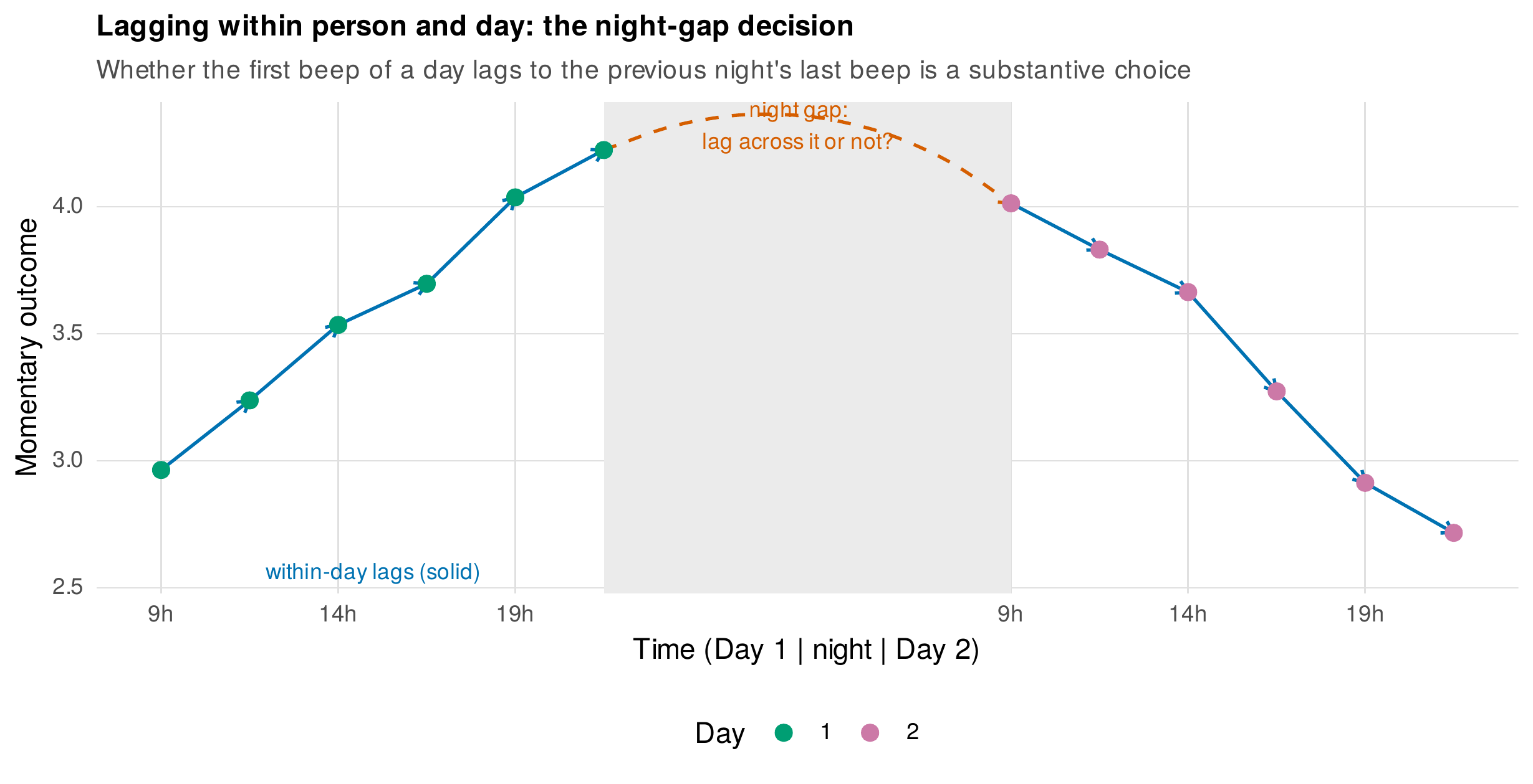
Note. Momentary observations across two days. Solid arrows are within-day lags; the dashed arrow across the shaded night is the decision the analyst must make explicitly, whether a state lags across the overnight gap. Recording the exact interval keeps the gap visible.
Common Pitfall • three derivations that fail silently
First, grouped-mutate leakage: forgetting ungroup() after a grouped mutate leaves the data grouped, so a later mutate(z = scale(x)) standardizes within each person rather than overall, with no warning. Always ungroup when the grouped operation is done. Second, lagging across persons: lag() applied to data that is not grouped by person, or not explicitly arranged, pairs the boundary observations of adjacent persons; always arrange and group_by(person) before lagging. Third, silent averaging over differing missingness: computing a scale mean with rowMeans(..., na.rm = TRUE) averages three items for one respondent and eight for another, so the “same” scale means different things across rows; decide and document a minimum-items rule instead.
5.6 The Reproducible Pipeline
The work of this chapter should flow in one direction, from raw data that is never modified, through a cleaning stage, to derived variables, to analysis, with each stage a separate script and the raw file treated as read-only. Figure 5.7 shows the flow. The raw export is archived untouched, so that any later question about a cleaning decision can be answered by rerunning the pipeline rather than by archaeology on an overwritten file. The cleaning script produces an intermediate clean file; the derivation script adds centered and lagged variables; the analysis scripts read only the derived file. This separation, combined with a package-version lockfile (renv) and, for larger projects, a pipeline manager (targets) that reruns only the stages affected by a change, makes the whole path from raw data to result reproducible by another person, or by yourself in a decade (Chapter 36 develops the reproducibility stack). Table 5.4 lists the minimum a codebook must contain to accompany an archived dataset.

Note. Each arrow is a separate, versioned script; each stage writes a new file rather than overwriting its input. The raw export is archived untouched so that every downstream decision can be reproduced from it.
Table 5.4. Minimum codebook fields and an archiving checklist.
| Codebook field | Archiving checklist (OSF or repository) |
|---|---|
| Variable name and label | Raw data archived read-only, with the export date |
| Type and units | Every cleaning and derivation script, versioned |
| Valid range / categories | The codebook and a data dictionary |
| Time metric and origin | A package-version lockfile (renv renv.lock) |
| Missing-value codes | A README stating the run order of scripts |
| Derivation (how computed) | A license and, for sensitive data, a de-identification note |
Note. Following the FAIR principles, findable, accessible, interoperable, reusable (Wilkinson et al., 2016), makes a dataset usable by others and by the future self who has forgotten every decision.
Software Note • helper packages versus pure tidyverse
Several packages target experience-sampling data cleaning specifically, offering ready functions for compliance summaries, careless-response indices, and lag construction; their availability and maintenance should be verified at the time of use, because such packages come and go. Nothing in this chapter, however, requires them: compliance is a count and a ratio, the longstring index is a short apply over item columns, and lags are dplyr::lag with explicit ordering, all pure tidyverse. Preferring the transparent, dependency-light idioms keeps a pipeline runnable years later, when a convenience package may have been archived. Where a maintained helper genuinely reduces error (careless-response detection has well-tested implementations), use it, but understand and record what it computes.
5.7 Reporting the Data Pipeline
Data preparation is reported in the Method section, and reviewers increasingly expect the decisions that move effect sizes to be stated rather than buried. A defensible data-preparation paragraph states four things: the compliance achieved and how it was computed, the screening rules and how many records each flagged, the exclusion rule actually applied and its sensitivity, and the derivations that produced the analysis variables. A model paragraph for the study of this chapter reads: “Of \(10{,}080\) scheduled prompts, \(7{,}342\) were answered (overall compliance \(72.8\%\); median per-person compliance \(73\%\), range \(58\)–\(85\%\)), computed from response timestamps. Responses completed in under three seconds or consisting of a single repeated value across all items were flagged as careless (\(26\) responses, \(0.4\%\)), and responses submitted more than fifteen minutes after the prompt were flagged as out of window (\(45\) responses, \(0.6\%\)); flagged responses were retained in the primary analysis and excluded in a sensitivity analysis, which did not alter the conclusions. Within-person deviations were computed by person-mean centering, and lagged predictors were constructed within person-days, with no carryover across the overnight gap.” Every clause records a decision made in this chapter, and the numbers come straight from the pipeline.
5.8 Common Misconceptions
Four beliefs cause avoidable damage. First, that cleaning is pre-scientific and needs no documentation: the decisions here, which cases to exclude, which clock to use, whether to lag across the night, routinely change effect sizes, and undocumented they cannot be reproduced or defended. Second, that long format is only for multilevel models: it is also the shape that modern plotting and much structural-equation tooling expect, and a long master file is the right source for any wide view. Third, that a compliance percentage is by itself a data-quality metric: the pattern of missingness matters more than its rate (Chapter 6), which is why compliance is visualized before it is summarized. Fourth, in answer to the frequent question “should I impute during cleaning?”: no, imputation is an analysis decision that depends on the model and the missingness mechanism (Chapter 6), and performing it during cleaning bakes an untested assumption into every downstream analysis.
Chapter Summary
Between a raw export and a fitted model lies a stretch of consequential, documentable work. Repeated-measures data live in wide and long shapes, and the analysis-ready form for this book is long, one row per person-occasion (Figure 5.1). Time is a variable to be built, not read off, and the choice among wave, study, clock, event, and developmental clocks determines whether change aligns with its cause (Figure 5.2). Merges are audited before they run, with anti_join checks and rename maps held as data, so that mismatched keys fail loudly rather than dropping rows silently. Intensive data are screened for compliance, viewed before it is summarized, and for careless responding, flagged rather than dropped. Derived variables, centered scores and lags, are computed with explicit grouping and ordering, and the night-gap lag is a substantive choice. The whole path runs one direction, from read-only raw data through clean and derived stages to analysis, archived with a codebook so that every decision can be reproduced.
Where to Go Next
The structures built here are consumed everywhere downstream: the missingness that compliance reveals is modeled in Chapter 6; the descriptive and graphical displays of Chapters 7 through 9 read the long format; the centered and lagged variables feed the multilevel and dynamic models of Chapters 13 and 23; the exact intervals preserved here enable the continuous-time models of Chapter 27; and the archiving discipline is completed in Chapter 36. The chapter’s single imperative is that every transformation between raw data and result is a decision to be documented and defended.
Exercises
- 5.1 Build a pipeline. Given the messy three-wave export in the
Examplesdata, produce an analysis-ready long file and a codebook. Verify your result against the provided checks (row counts, key uniqueness, value ranges). - 5.2 Three clocks. For a dataset of your choice, construct wave, study-day, and event-time variables. State the research question each clock serves, and plot the same outcome against all three.
- 5.3 Night-gap lags. Implement a within-day lag and an across-night lag on
affect_ema. Fit a simple model of negative affect on its own lag under each rule, and report how the autoregressive coefficient differs. - 5.4 Write the paragraph. Using the pipeline output, write the data-preparation and compliance paragraph for
affect_emafollowing Section 5.7. - 5.5 Break the join. The provided wave files contain planted merge bugs (a drifting name, a duplicated key, an orphaned identifier). Find each with an audit, and state what a naive
left_joinwould have done.
References
Broman, K. W., & Woo, K. H. (2018). Data organization in spreadsheets. The American Statistician, 72(1), 2–10. https://doi.org/10.1080/00031305.2017.1375989
Curran, P. G. (2016). Methods for the detection of carelessly invalid responses in survey data. Journal of Experimental Social Psychology, 66, 4–19. https://doi.org/10.1016/j.jesp.2015.07.006
Curran, P. J., & Hussong, A. M. (2009). Integrative data analysis: The simultaneous analysis of multiple data sets. Psychological Methods, 14(2), 81–100. https://doi.org/10.1037/a0015914
Meade, A. W., & Craig, S. B. (2012). Identifying careless responses in survey data. Psychological Methods, 17(3), 437–455. https://doi.org/10.1037/a0028085
Wickham, H. (2014). Tidy data. Journal of Statistical Software, 59(10), 1–23. https://doi.org/10.18637/jss.v059.i10
Wickham, H., Çetinkaya-Rundel, M., & Grolemund, G. (2023). R for data science: Import, tidy, transform, visualize, and model data (2nd ed.). O’Reilly Media.
Wilkinson, M. D., Dumontier, M., Aalbersberg, I. J., Appleton, G., Axton, M., Baak, A., Blomberg, N., Boiten, J.-W., da Silva Santos, L. B., Bourne, P. E., Bouwman, J., Brookes, A. J., Clark, T., Crosas, M., Dillo, I., Dumon, O., Edmunds, S., Evelo, C. T., Finkers, R., … Mons, B. (2016). The FAIR Guiding Principles for scientific data management and stewardship. Scientific Data, 3, Article 160018. https://doi.org/10.1038/sdata.2016.18