Chapter 6
Missing Data and Attrition in Longitudinal Research
Longitudinal data are missing-data problems by construction. Participants skip waves, miss beeps, leave the study, and answer some items but not others, so that the rectangular data matrix a method assumes is almost never the matrix a study collects. This chapter is placed deliberately before the estimation parts of the book, because the way missingness is handled is not a nuisance step applied after the real analysis but a modeling decision that determines whether the real analysis is valid at all. The central claim is that the older repairs most researchers were taught, deleting incomplete cases and carrying the last value forward, are not conservative defaults but active sources of bias, and that two modern procedures, full-information maximum likelihood and multiple imputation, are both principled and, for the multilevel and intensive data of this book, within reach.
Learning Objectives
After working through this chapter, you should be able to: (1) state Rubin’s mechanisms, missing completely at random, missing at random, and missing not at random, as precise claims about the joint distribution of the data and the missingness, and explain why the taxonomy governs the validity of ignoring missingness rather than describing its causes; (2) diagnose monotone and intermittent patterns and conduct an informative attrition analysis without overselling it as proof of ignorability; (3) explain, with directional intuition, why listwise deletion and last-observation-carried-forward bias longitudinal estimates; (4) fit a model by full-information maximum likelihood and say exactly what likelihood is being maximized; (5) run multiple imputation appropriate to the data structure, including multilevel imputation for nested and intensive data; (6) choose between full-information maximum likelihood and multiple imputation on principled grounds; (7) carry out and report at least two missing-not-at-random sensitivity analyses, including a tipping-point analysis; and (8) use planned missingness designs to reduce respondent burden by design.
6.1 The Anatomy of Longitudinal Missingness
Missingness in repeated measures is not one phenomenon but several, and naming the pattern is the first step because different patterns admit different remedies. Unit nonresponse is the loss of an entire person, who is sampled but never measured or who withdraws before the first wave. Wave nonresponse is the loss of an entire occasion for some persons, as when a follow-up assessment is missed but the person returns later. Monotone dropout, or attrition, is the pattern in which a person, once absent, is absent for every subsequent occasion; it is the dominant pattern in panel studies and clinical trials, and its monotone structure simplifies both imputation and modeling. Intermittent missingness is the non-monotone pattern in which persons drift in and out, present at some occasions and absent at others, which is characteristic of experience-sampling and diary designs. Item missingness is the loss of particular questions within an otherwise completed assessment, and prompt-level missingness in intensive longitudinal designs is the failure to respond to a scheduled beep at all. Figure 6.1 displays six of these archetypes as person-by-occasion matrices, the display that should precede any numerical summary of missingness because it reveals structure that a single completion rate conceals.
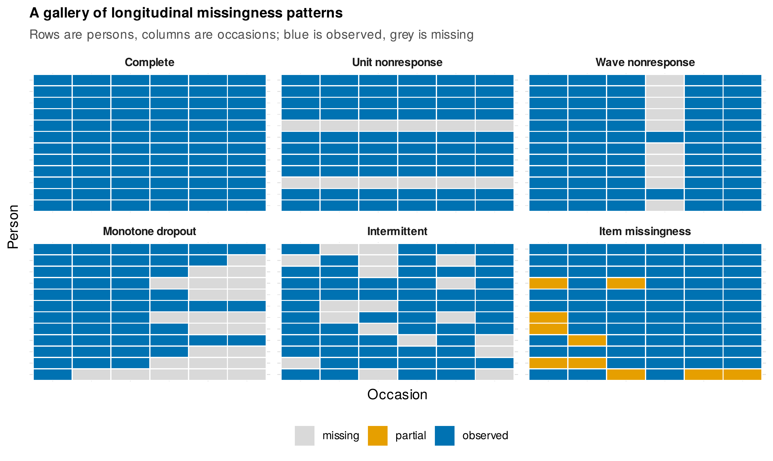
Note. Rows are persons, columns are occasions; blue cells are observed, grey cells are missing, and partial shading marks item-level loss within a completed assessment. Monotone dropout, in which absence is absorbing, is the typical pattern of panel and trial attrition; intermittent missingness is typical of intensive designs. The pattern determines which imputation and estimation strategies apply.
The consequential distinction, however, is not the pattern but the mechanism, the probabilistic relationship between the chance that a value is missing and the values of the data, both seen and unseen. Rubin’s (1976) taxonomy formalizes this relationship. Let \(Y\) denote the complete data, partitioned into the observed part \(Y_{\mathrm{obs}}\) and the missing part \(Y_{\mathrm{mis}}\), and let \(M\) be the matrix of missingness indicators recording which entries are present. The mechanism is the conditional distribution \(P(M \mid Y_{\mathrm{obs}}, Y_{\mathrm{mis}}, \phi)\), governed by parameters \(\phi\). Data are missing completely at random (MCAR) when missingness is independent of the data entirely, \(P(M \mid Y_{\mathrm{obs}}, Y_{\mathrm{mis}}, \phi) = P(M \mid \phi)\), so that the observed cases are a simple random subsample of the complete cases. Data are missing at random (MAR) when missingness may depend on the observed values but, given them, not on the missing values, \(P(M \mid Y_{\mathrm{obs}}, Y_{\mathrm{mis}}, \phi) = P(M \mid Y_{\mathrm{obs}}, \phi)\). Data are missing not at random (MNAR) when, even after conditioning on everything observed, the probability of missingness still depends on the unseen values themselves. Figure 6.2 renders the three mechanisms as dependence diagrams, and Table 6.1 states each definition alongside what remains valid under it.
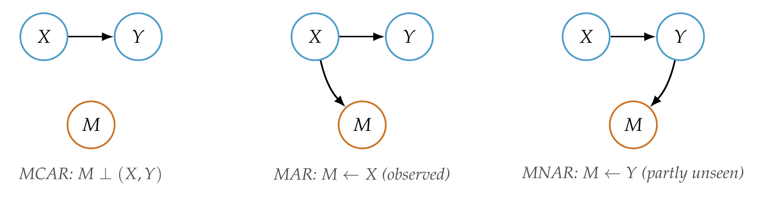
Note. \(X\) is a fully observed covariate, \(Y\) is a partially observed outcome, and \(M\) is the missingness indicator for \(Y\). Under MCAR no arrow reaches \(M\) from the data. Under MAR the arrow into \(M\) originates only from observed information (\(X\), and observed values of \(Y\)). Under MNAR the arrow into \(M\) originates from \(Y\) itself, whose relevant values are partly unseen, which is why the assumption cannot be checked from the data at hand.
Three points about this taxonomy are routinely misunderstood and worth stating plainly. First, the labels describe the validity of ignoring the missingness process, not the causes of missingness in any everyday sense; MAR does not mean the missingness is haphazard or benign, only that its dependence runs through quantities that were recorded. Second, MAR is untestable against MNAR using the observed data, because the two mechanisms make identical predictions about \(Y_{\mathrm{obs}}\) and differ only in their dependence on \(Y_{\mathrm{mis}}\), which by definition is not available; any claim that a dataset “is MAR” is an assumption, defensible or not, never a finding. Third, MCAR alone is partially testable, and Little’s (1988) test provides an omnibus check by comparing the observed-variable means across missingness patterns, but its non-significance is weak evidence, sensitive to power and to the specific alternative, and it must never be read as licensing the far stronger MAR assumption the analysis actually relies on. The practical reframing for students is to replace the question “which label fits my data” with the question “what must I be willing to believe for my chosen method to be valid,” because the second question is answerable and leads directly to sensitivity analysis when the belief is uncertain.
Table 6.1. Rubin’s missingness mechanisms and their consequences.
| Mechanism | Definition | Testable? | Valid under it |
|---|---|---|---|
| MCAR | \(P(M \mid Y_{\mathrm{obs}}, Y_{\mathrm{mis}}) = P(M)\); missingness independent of all data | Partially (Little’s test) | Listwise deletion (unbiased, inefficient); FIML; MI |
| MAR | \(P(M \mid Y_{\mathrm{obs}}, Y_{\mathrm{mis}}) = P(M \mid Y_{\mathrm{obs}})\); depends only on observed data | No (untestable vs. MNAR) | FIML; MI (both consistent); listwise generally biased |
| MNAR | Depends on \(Y_{\mathrm{mis}}\) even given \(Y_{\mathrm{obs}}\) | No | No method valid without modeling \(M\); requires sensitivity analysis |
Note. Under MAR, likelihood-based estimation with the missingness process left unmodeled is valid provided the variables driving missingness are included in the model, the property Rubin termed ignorability. “Valid” means consistent for the target parameter; efficiency still varies across methods.
6.2 What the Bad Methods Do
The default repairs taught to a generation of researchers are listwise deletion, which discards any person with an incomplete record, and last-observation-carried-forward (LOCF), which fills a missing value with the person’s most recent observed value. Both are widely believed to be conservative. Both are, in the longitudinal setting, actively misleading, and the argument is worth making precisely because the belief is so entrenched.
Listwise deletion is unbiased only under MCAR, and even then it is wasteful, because in a study with several occasions the probability that a person is complete on every one can be small, so that a design collecting hundreds of person-occasions is reduced to the minority who never missed. Under MAR the deletion is not merely inefficient but biased, because the completers are a selected subsample, and in longitudinal health and clinical research the selection is rarely benign: completers are systematically the healthier, the more adherent, and the more improved, so that a growth curve fitted to completers describes the trajectory of the people who stayed, not the population that was enrolled. There is one nuance that keeps complete-case analysis alive in specific regression settings, that when missingness depends only on covariates that are themselves fully observed and included as predictors, the complete-case regression coefficient can remain unbiased; but this exception concerns covariate-driven missingness in a conditional model, not the outcome-driven attrition that dominates longitudinal studies, and it should not be generalized into a defense of the method.
LOCF is worse, because it does not merely select a subsample but fabricates data, and the fabrication has a direction. In a study where the typical trajectory is improvement, as in the therapy trial of this chapter, carrying forward the last observed value freezes each dropout at their pre-dropout severity, which asserts, with no evidence, that improvement stopped at the moment of departure. If dropout is concentrated among non-responders, LOCF preserves their high symptom scores and drags the treatment-group mean upward, attenuating the estimated benefit; if dropout is concentrated among responders who leave because they are well, LOCF understates their continued gains. Either way the method replaces a missing value with a value known to be systematically wrong, and its reputation for conservatism is an accident of the particular trials in which it happened to bias toward the null. Mean imputation, filling a gap with the sample or wave mean, shares the fabrication and adds a second defect, the attenuation of variance and of every covariance, because the imputed values carry no dispersion and lie exactly on the mean; a single-value regression imputation improves the point but still injects false certainty by treating imputed values as if observed.
Figure 6.3 is the chapter’s signature demonstration and the reason to invest in the alternatives. It reports the estimated treatment-by-time interaction, the difference in symptom slope between arms, from a known-truth simulation in which the true effect is \(-0.40\) symptom points per week and monotone dropout is imposed under each of the three mechanisms; the full simulation is the shipped script ch06_missing_sims_V01.R. The lesson is stark and has three layers. Under MCAR, where deletion is supposed to be safe, listwise deletion does recover the truth (\(-0.39\)) but at a large cost in precision, while LOCF (\(-0.32\)) and mean imputation (\(-0.25\)) are already biased toward zero, because their fabricated values distort the very slopes the model estimates. Under MAR the naive methods deteriorate further while the principled methods hold. Under MNAR, the hardest case, mean imputation collapses entirely (\(-0.07\)), listwise and LOCF are badly biased, and even here full-information maximum likelihood recovers the truth almost exactly (\(-0.40\)) with multiple imputation close behind (\(-0.35\)), because the pre-dropout trajectory, which both methods use in full, carries most of the information about the slope. The MNAR result is not a promise that likelihood methods repair MNAR in general, they do not, but a demonstration that discarding or fabricating data forfeits information that principled methods retain, and it motivates the sensitivity analysis of Section 6.6 rather than substituting for it.
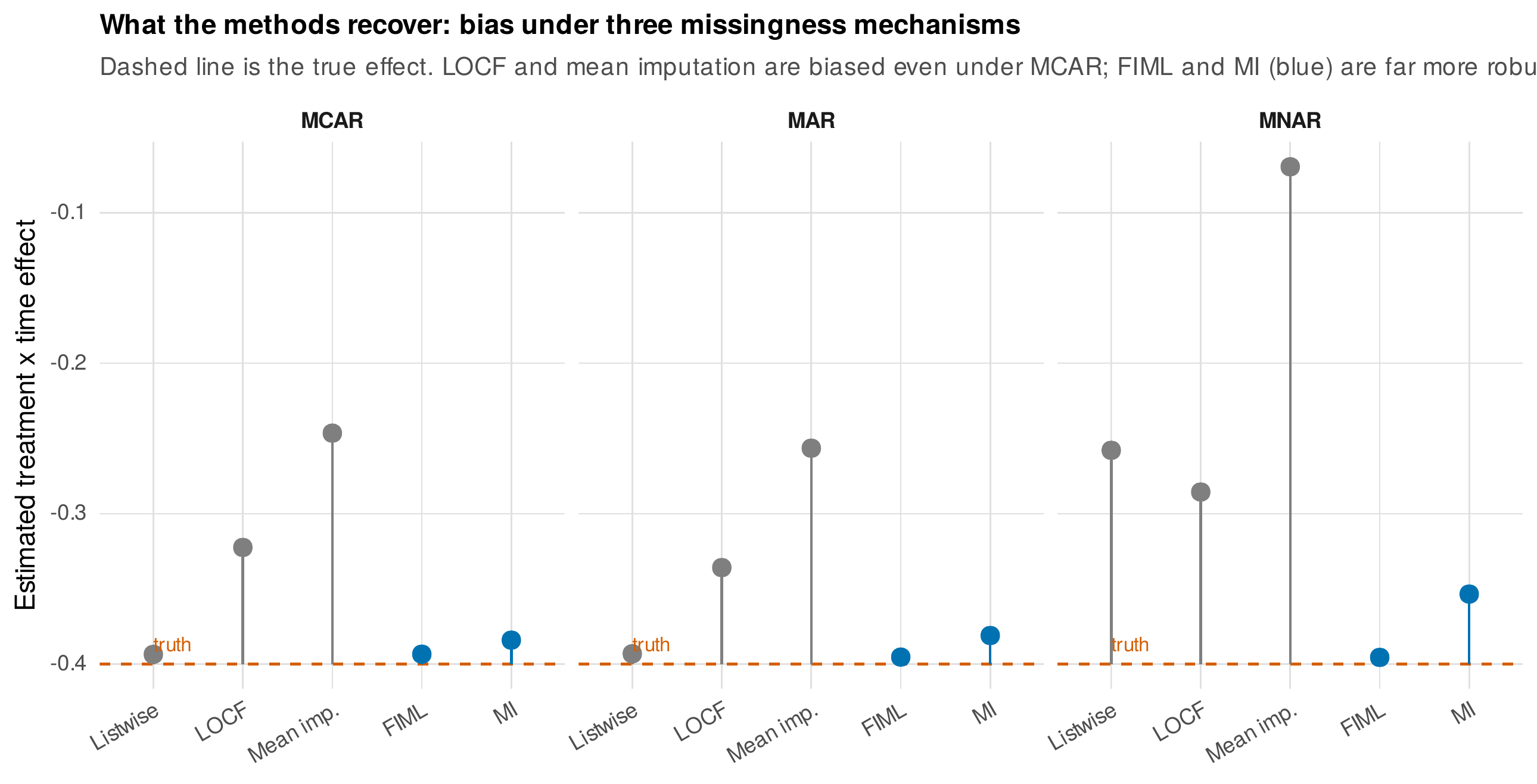
Note. Each point is the average estimated treatment-by-time interaction across 100 replications; the dashed line is the true effect (\(-0.40\)). Grey points are the naive methods (listwise, LOCF, mean imputation); blue points are the principled methods (FIML, MI). LOCF and mean imputation are biased toward zero even under MCAR, where deletion is nominally valid. FIML and MI remain close to the truth across all three mechanisms; the residual MNAR gap for MI, and its treatment in Section 6.6, are the honest limits of what data alone can do.
6.3 Full-Information Maximum Likelihood
The first principled alternative reframes the problem. Rather than repairing the data so that a complete-data method can run, full-information maximum likelihood (FIML), also called direct maximum likelihood, changes the estimator so that incomplete records need no repair. The idea rests on a factorization of the likelihood. Under an ignorable mechanism, the likelihood of the parameters given the observed data can be written without reference to the missingness model, so that each person contributes to the likelihood through the density of exactly the variables that person has, evaluated at the parameters of the full model. A person measured on all occasions contributes the full multivariate density; a person measured on a subset contributes the corresponding marginal density; no value is filled in, and no case is deleted, because the estimator simply sums whatever information each person supplies. The Foundations box states the factorization and the ignorability condition that licenses it.
Foundations Box • The observed-data likelihood and ignorability
Write the joint model for the data and the missingness as \(P(Y_{\mathrm{obs}}, Y_{\mathrm{mis}}, M \mid \theta, \phi) = P(Y_{\mathrm{obs}}, Y_{\mathrm{mis}} \mid \theta)\, P(M \mid Y_{\mathrm{obs}}, Y_{\mathrm{mis}}, \phi)\), where \(\theta\) indexes the data model and \(\phi\) the missingness model. The observed-data likelihood integrates over the missing values, \(L(\theta, \phi \mid Y_{\mathrm{obs}}, M) \propto \int P(Y_{\mathrm{obs}}, Y_{\mathrm{mis}} \mid \theta)\, P(M \mid Y_{\mathrm{obs}}, Y_{\mathrm{mis}}, \phi)\, dY_{\mathrm{mis}}\). When the mechanism is MAR, \(P(M \mid Y_{\mathrm{obs}}, Y_{\mathrm{mis}}, \phi) = P(M \mid Y_{\mathrm{obs}}, \phi)\) factors out of the integral, leaving \(L(\theta \mid Y_{\mathrm{obs}}) \propto \int P(Y_{\mathrm{obs}}, Y_{\mathrm{mis}} \mid \theta)\, dY_{\mathrm{mis}} = P(Y_{\mathrm{obs}} \mid \theta)\). If in addition the parameters \(\theta\) and \(\phi\) are distinct, inference about \(\theta\) can proceed from the observed-data density \(P(Y_{\mathrm{obs}} \mid \theta)\) alone, ignoring the missingness model entirely. This is Rubin’s ignorability, and it is the formal reason that a correctly specified likelihood analysis of the observed data is valid under MAR.
This factorization also explains a fact that is usually stated as a black-box convenience, that multilevel and mixed-effects models “handle unbalanced data automatically.” The mixed model is estimated by maximizing exactly the observed-data likelihood above, so a person with three of five occasions simply contributes a three-dimensional density; there is no deletion and no imputation because the estimator was never expressed in terms of a complete rectangle. The frequently missed condition is precisely stated in the ignorability derivation: validity holds when the missingness depends only on quantities in the model. If attrition depends on a baseline covariate, that covariate must be in the model for the analysis to inherit the MAR guarantee, which is why a mixed model that omits the predictors of dropout is not automatically protected. In the structural equation framework the same estimator is invoked in lavaan with the argument missing = "ml", and its reach is extended by auxiliary variables, correlates of the outcome or of missingness that are not part of the substantive model but are added, through a saturated-correlates specification, so that the MAR conditioning set is enriched and the estimates are both less biased and more efficient (Collins et al., 2001). The limits of FIML are also worth stating: it assumes the outcome distribution it is given, so nonnormality calls for robust corrections; it addresses missingness on the modeled variables, not on exogenous predictors treated as fixed; and it can incorporate auxiliary information only by bringing those variables into the estimated model.
6.4 Multiple Imputation
The second principled alternative separates the treatment of missingness from the analysis. Multiple imputation (MI) replaces each missing value not once but \(m\) times, drawing from the posterior predictive distribution of the missing data given the observed data, to produce \(m\) complete datasets that differ only in their imputed values. The substantive analysis is run on each completed dataset, and the \(m\) sets of results are combined by Rubin’s rules, which are the arithmetic that makes the procedure honest. The pooled point estimate is the average of the \(m\) estimates, \(\bar{Q} = \frac{1}{m}\sum_{j=1}^{m} \hat{Q}_j\). The total variance has two parts, \(T = \bar{U} + (1 + 1/m)\,B\), where \(\bar{U} = \frac{1}{m}\sum_j U_j\) is the average within-imputation sampling variance, the ordinary uncertainty that would remain if the data were complete, and \(B = \frac{1}{m-1}\sum_j (\hat{Q}_j - \bar{Q})^2\) is the between-imputation variance, the extra uncertainty that the missingness itself contributes. The factor \((1 + 1/m)\) corrects for using a finite number of imputations. The crucial feature is \(B\): because the imputations vary, the between-imputation variance is nonzero, and the pooled standard error is inflated to reflect the real cost of the missing data, which is exactly the certainty that single imputation counterfeits. The fraction of that total variance due to missingness, the fraction of missing information (FMI), governs how many imputations are needed and how much efficiency is lost.
The validity of MI rests on a condition that is easy to violate in practice, congeniality, the requirement that the imputation model be at least as rich as the analysis model. Every feature the analysis will estimate must be preserved by the imputation: if the analysis includes an interaction, the imputation model must include it, or the imputed values will be drawn from a distribution in which the interaction is absent and the pooled estimate will be attenuated toward zero; the same holds for nonlinear terms, for the outcome when imputing predictors, and for the clustering structure discussed below. Table 6.2 is a construction checklist for the imputation model. In R the standard implementation is mice (van Buuren & Groothuis-Oudshoorn, 2011), which imputes by fully conditional specification, cycling through the incomplete variables and imputing each from a regression on the others, with predictive mean matching as a robust default that draws imputed values from observed cases and so respects the empirical distribution. The workflow has a discipline: the predictor matrix is set deliberately rather than left at its default, the number of imputations is chosen larger than the historically cited five, following the modern advice to scale \(m\) to the fraction of missing information (von Hippel, 2020), and the imputations are inspected before use. Figure 6.4 shows the essential diagnostic, an overlay of the observed and imputed densities: the imputed values should be plausible relative to the observed, neither identical, which would signal that the imputation added nothing, nor wildly displaced, which would signal a misspecified imputation model.
Table 6.2. Imputation-model construction checklist (congeniality).
| Feature of the analysis | Requirement on the imputation model |
|---|---|
| Interaction terms | Include the product, or impute within subgroups, so the association is preserved. |
| Nonlinear terms (e.g., \(x^2\)) | Impute the transformed quantity (passive imputation) or include it as a predictor. |
| The outcome \(Y\) | Include \(Y\) when imputing predictors; omitting it biases associations toward zero. |
| Clustering / nesting | Use a multilevel imputation model; flat imputation distorts variance components (Fig. 6.5). |
| Auxiliary variables | Add correlates of missingness or of \(Y\) to strengthen the MAR conditioning set. |
| Derived scale scores | Impute at the item level where feasible, then form scores (passive imputation). |
Note. The governing principle is that the imputation model must be at least as general as the analysis model. Any structure the analysis will estimate but the imputation omits is systematically erased from the completed data.
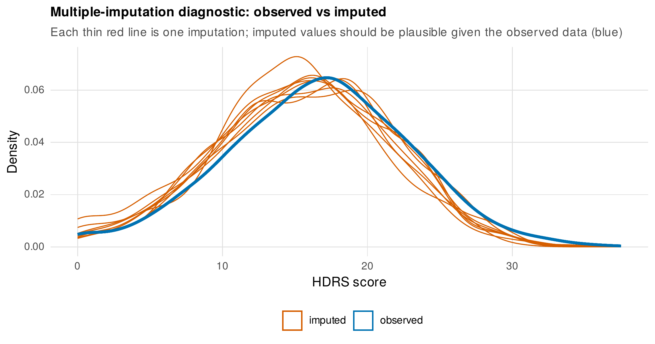
Note. The thick blue curve is the density of the observed HDRS values; each thin red curve is the density of the imputed values in one of eight completed datasets. Imputed values that track the observed distribution, as here, are a necessary (not sufficient) sign of a reasonable imputation model. Systematic displacement of the red curves would indicate misspecification.
The section that distinguishes this book from a standard treatment concerns multilevel multiple imputation, because the longitudinal and intensive data of interest are nested, occasions within persons, and flat imputation that ignores the nesting does measurable damage. The clearest casualty is the intraclass correlation (ICC), the proportion of variance that lies between persons, which is the quantity that defines how much a design gains from its repeated measurements. Figure 6.5 makes the point on the experience-sampling data: the true ICC of momentary negative affect is \(0.36\), but imputing the missing beeps with a flat model that treats all observations as exchangeable, ignoring the person level, nearly halves it to \(0.20\), because pooling across persons blends each person’s values toward the grand mean and destroys the between-person separation. A multilevel imputation that models the person as a cluster, here mice with the 2l.pan method, recovers the truth (\(0.38\)). The same distortion afflicts within-person and between-person regression coefficients whenever they are imputed flat, which is why congeniality in nested data requires a nested imputation model. The practical choices are two: for a small number of waves, wide-format imputation with occasions as separate columns can preserve the covariance structure adequately; for the long series of intensive designs, a genuine multilevel imputation, through the joint-modeling tools (jomo, mitml) or the multilevel methods within mice, is required, with the honest caveat that random-slope structures remain difficult to impute congenially and that the fully conditional and joint-modeling approaches trade different assumptions. The pooling of multilevel results follows the same Rubin arithmetic, implemented for mixed models and lavaan in the mitml and semTools ecosystems, whose exact function names should be verified at the time of use because the tooling evolves. Table 6.3 summarizes when to reach for which strategy.
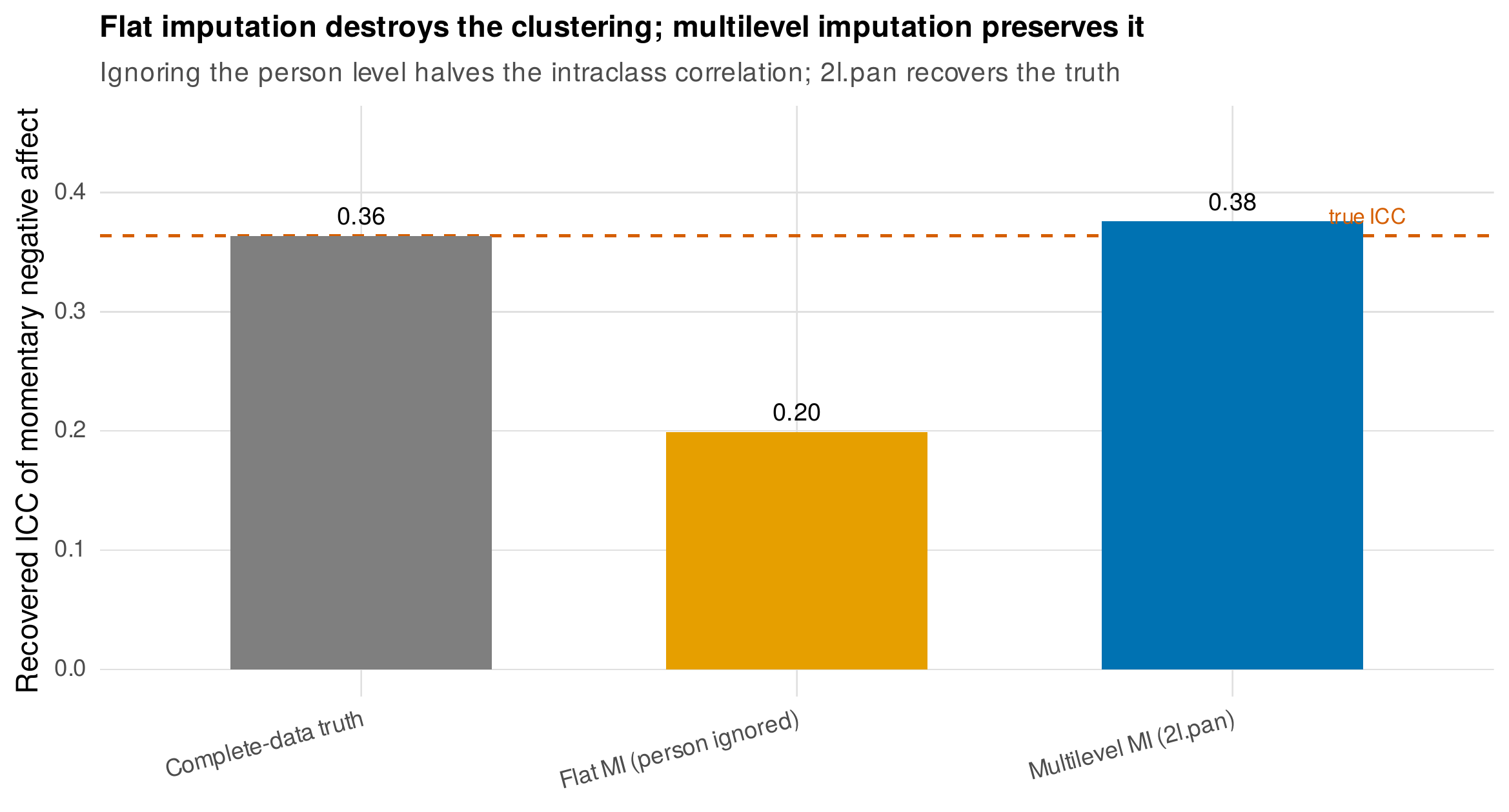
Note. The dashed line is the true ICC of momentary negative affect in the experience-sampling data (\(0.36\)). Flat imputation, which ignores the person level, nearly halves the recovered ICC to \(0.20\); multilevel imputation with 2l.pan recovers it (\(0.38\)). Because the ICC governs the information content of a repeated-measures design, its distortion propagates to every variance-partitioning and cross-level result downstream.
Table 6.3. A guide to method by situation.
| Situation | Preferred approach | Notes |
|---|---|---|
| Mixed model, missingness on outcome only | FIML (direct ML) | Automatic in lmer/lavaan; include dropout predictors as covariates. |
| Missingness on predictors | MI | FIML cannot impute exogenous \(x\); MI can. |
| Strong auxiliary variables available | MI, or FIML with saturated correlates | Auxiliaries enrich the MAR conditioning set. |
| Few waves, nested | Wide-format MI or FIML | Wide MI preserves the occasion covariance. |
| Intensive / many occasions, nested | Multilevel MI (2l.pan, jomo) | Flat MI distorts the ICC (Fig. 6.5). |
| Categorical or count outcomes | MI with matching methods, or model-based ML | Check congeniality with the analysis link. |
| Suspected MNAR | Any principled base + sensitivity analysis | No method is valid without modeling \(M\) (Section 6.6). |
Note. FIML and MI are asymptotically equivalent when the imputation and analysis models are congenial and use the same information; the choice is practical, turning on where the missingness sits and what auxiliary information is available.
For the intensive-data analyst there is a final, orienting question, whether to impute at all. When the analysis is a multilevel or dynamic model estimated by maximum likelihood, the observed responses can often be modeled directly, so that imputation is unnecessary for the outcome and is reserved for missingness on covariates, for auxiliary-variable inclusion, or for methods, such as some network and vector-autoregressive models (Chapters 25 and 28), that require complete series as input. The decision is not dogma but a matter of matching the tool to the missingness: model the outcome under ML when the model permits, impute when the structure of the problem or the analysis method demands complete data.
6.5 Attrition Analysis and Reporting
Before any modeling, a longitudinal study owes its readers a description of who left and when. The weak version of this, a single dropout percentage, discards the temporal structure that matters; the informative version treats retention as a process. Figure 6.6 plots the proportion still in the therapy trial against week for each arm, which is a survival display (the formal machinery of which is Chapter 29), and it communicates at a glance what a rate cannot: whether attrition is early or late, steady or clustered, and whether it differs by condition. In the trial shown, retention declines steadily in both arms to roughly \(56\%\) at the final week, with the arms tracking closely, which is itself informative because differential dropout between conditions is a specific threat that this display would expose.
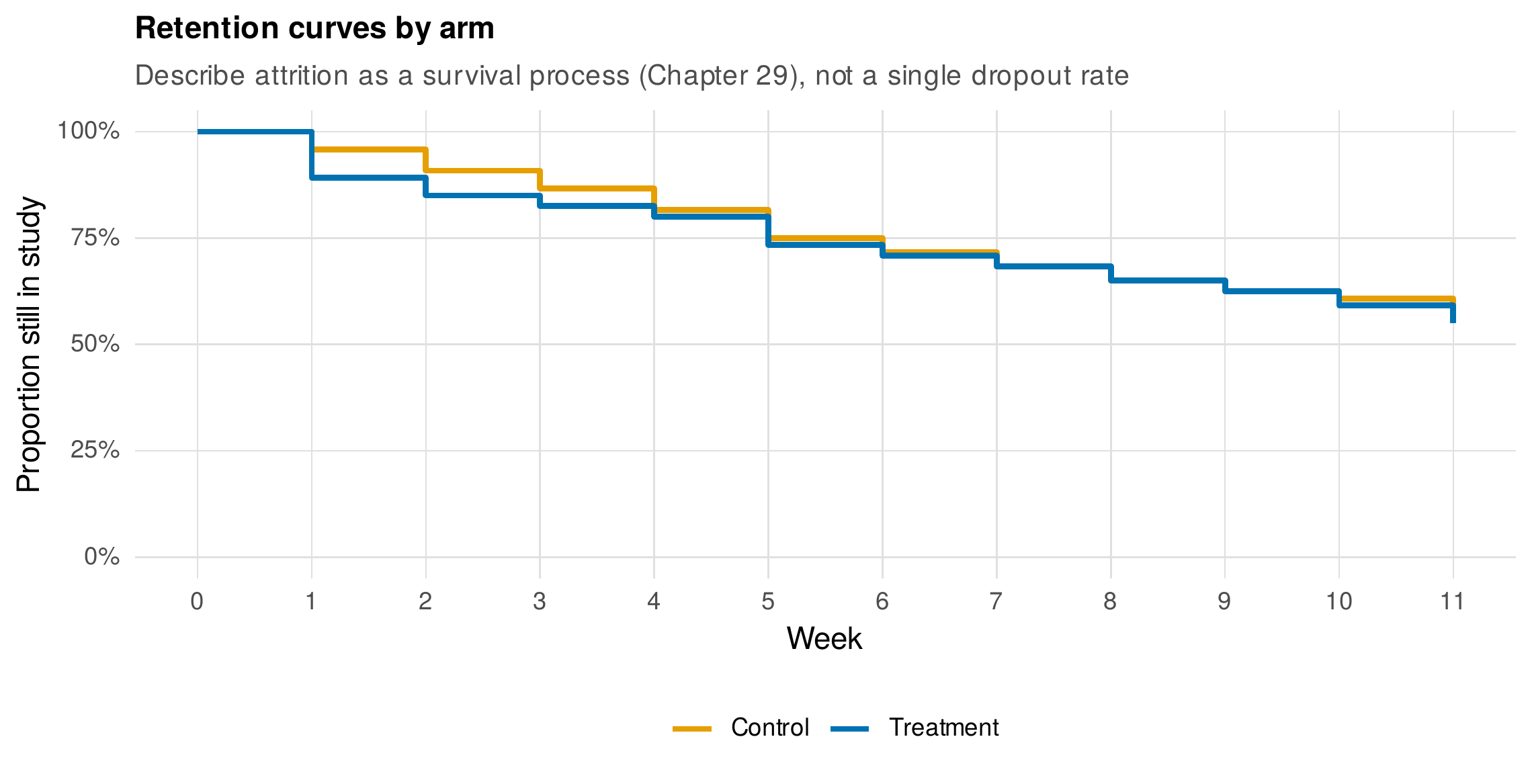
Note. The proportion of each arm still contributing data is plotted against week. Describing attrition as a retention process, rather than a single end-of-study dropout rate, exposes its timing and any between-arm differential, both of which bear on the plausibility of the ignorability assumption.
The attrition analysis proper compares those who left with those who stayed, and it must compare them on two things, not one. Comparison on baseline characteristics, demographics and initial status, is standard but insufficient, because two people identical at baseline may differ sharply in their trajectory before one of them drops out. The longitudinal-specific comparison is therefore on the trajectory so far: whether dropouts were, in the occasions they did provide, improving or worsening relative to completers. A finding that dropouts had steeper pre-dropout decline, or higher pre-dropout severity, does not prove MNAR, but it identifies the observed quantities on which missingness depends, which is exactly the information that, once included in the model, converts a threatening MNAR story into a defensible MAR one. This reframes the purpose of the attrition analysis: it is not a test to be passed, a nonsignificant difference declared as proof of randomness, but a search for the predictors of missingness that the analysis must then incorporate. Where those predictors cannot be brought into the model, an alternative frame is inverse-probability weighting, which reweights the observed cases by the inverse of their estimated probability of being observed, upweighting the underrepresented; it is the natural companion to the marginal models of Chapter 12 and carries its own fragility under misspecification of the weight model. Reporting should follow the CONSORT extension for longitudinal and cluster designs, with a participant-flow diagram that accounts for every enrolled person at every wave, and the language templates of Section 6.9 make the expected paragraph concrete.
6.6 MNAR Sensitivity Analysis
When missingness may depend on the unseen values themselves, no analysis of the observed data can be known to be correct, and the honest response is not to search for the one MNAR model that rescues the result but to ask how much the conclusion would have to be wrong before it changed. This is the logic of sensitivity analysis, and its modern, practical form is the pattern-mixture model with a delta adjustment. The idea is transparent: impute the missing values under MAR, then deliberately shift the imputed values for the dropouts by a sensitivity parameter \(\delta\), representing the assumption that those who left did systematically worse (or better) than their observed data predicted, refit the model, and trace the estimate as \(\delta\) grows. The result is a tipping-point analysis, which locates the value of \(\delta\) at which the substantive conclusion, here the significance of the treatment effect, is overturned, and then asks whether a departure of that magnitude is clinically or psychologically plausible.
Figure 6.7 carries out this analysis for the therapy trial. Under MAR (\(\delta = 0\)) the estimated treatment-by-time effect is clearly nonzero and favorable, and as the dropouts in the treatment arm are assumed to have deteriorated by increasing amounts, the estimated advantage shrinks and its confidence interval widens. The tipping point is at approximately \(\delta = 5.6\) HDRS points: only if the treatment-arm dropouts are assumed to have ended, on average, nearly six depression-scale points worse than their pre-dropout trajectory predicted, a substantial and arguably implausible unravelling, does the treatment effect lose significance. This is a strong sensitivity result, because it converts an untestable assumption into a quantified, interpretable margin, and it is reported not as a weakness but as evidence of robustness. The alternative family, the selection model of Diggle and Kenward (1994), instead specifies an explicit model for the probability of dropout as a function of the possibly-missing current value and estimates it jointly with the outcome model; it is conceptually elegant but its identification rests almost entirely on distributional assumptions rather than on information in the data, so its estimates are fragile and it is best used to probe, not to settle. The doctrine that a principled analysis reports a range of results under a range of plausible missingness assumptions, rather than a single number under an unexamined one, is now the standard recommended by methodological consensus for clinical trials (National Research Council, 2010), and the shared-parameter and joint longitudinal-survival models of Chapter 29 are its most ambitious expression.
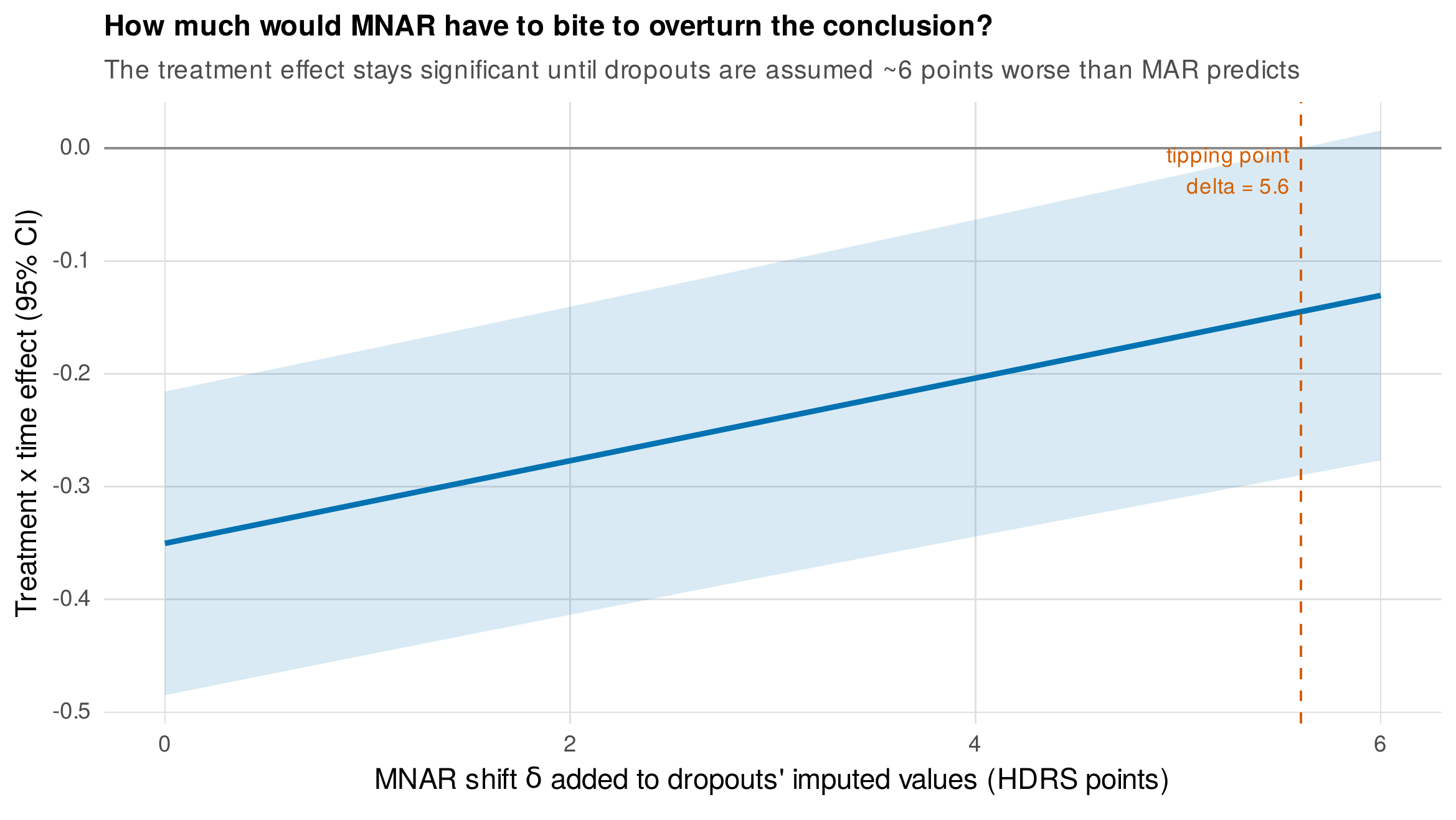
Note. The estimated treatment-by-time effect and its 95% confidence interval are plotted against the MNAR sensitivity parameter \(\delta\), the number of HDRS points by which treatment-arm dropouts are assumed to exceed their MAR-predicted values. The conclusion remains significant until \(\delta \approx 5.6\), a large assumed departure, which quantifies the robustness of the finding to plausible MNAR violations.
6.7 Planned Missingness
Missingness is usually a problem inflicted on a study, but it can also be a tool a study chooses, and planned missingness designs exploit the machinery of this chapter to reduce respondent burden by design (Graham et al., 2006). In a three-form design, the item pool is divided into a common core administered to everyone and three additional blocks, and each respondent receives the core plus two of the three blocks, so that every respondent answers two-thirds of the items and every pair of blocks is jointly observed in some respondents, which is exactly the coverage that lets multiple imputation or FIML recover the full covariance structure. Figure 6.8 shows the schematic. The missingness so induced is MCAR by construction, because block assignment is randomized and unrelated to any response, so the strong assumptions that trouble unplanned missingness simply do not arise, and the cost is a modest, quantifiable loss of efficiency in exchange for a large reduction in the length of any one questionnaire. In intensive longitudinal designs the same logic supports item rotation across beeps, presenting a subset of items at each prompt to keep the momentary burden low while accumulating full coverage across the day. The cautions are real: planned missingness interacts badly with small samples, where the efficiency loss bites hardest, and it presumes the analysis will use a principled missing-data method, so a three-form design analyzed by listwise deletion would discard its own rationale.
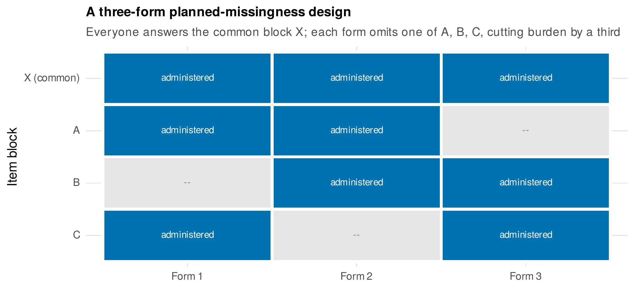
Note. Every respondent answers the common block \(X\); the three forms each omit one of blocks \(A\), \(B\), and \(C\). Each respondent thus completes two-thirds of the items, and every block pair is jointly observed in some forms, so the full covariance is recoverable by FIML or MI. The induced missingness is MCAR by design.
6.8 Running Missing-Data Analyses in R
The worked example takes the therapy trial through the full arc, from describing attrition to fitting the growth model under a principled method to probing MNAR. The data are the therapy_rct set, \(240\) patients across two arms measured weekly for twelve weeks, with monotone dropout affecting \(44\%\) of patients and leaving \(75\%\) of person-weeks observed. The first task is to describe retention rather than to summarize it with a single number.
library(dplyr); library(tidyr); library(ggplot2); library(lme4)

rct <- readRDS("Examples/data/therapy_rct.rds")

# --- Attrition described as a retention process, by arm ---
retention <- rct %>%
  group_by(arm, week) %>%
  summarise(retained = mean(!is.na(hdrs)), .groups = "drop")

# --- Attrition analysis: do dropouts differ from completers? ---
completer <- rct %>% group_by(patient_id) %>%
  summarise(complete = all(!is.na(hdrs)), .groups = "drop")
rct <- left_join(rct, completer, by = "patient_id")
rct %>% filter(week == 0) %>%                 # baseline comparison
  group_by(complete) %>%
  summarise(baseline_hdrs = mean(hdrs), n = n())
The retention curves (Figure 6.6) and the baseline comparison together form the attrition analysis; the baseline comparison should be supplemented by a comparison of the pre-dropout slope, which is the longitudinal-specific check. The growth model is then fitted by direct maximum likelihood, which for a mixed model is automatic: lmer maximizes the observed-data likelihood, so passing the incomplete long-format data fits the model under FIML with no special argument, provided the predictors of dropout are in the model.
# --- FIML via the mixed model: no deletion, no imputation ---
fit_fiml <- lmer(hdrs ~ week * arm + (1 + week | patient_id),
                 data = rct)                  # observed rows only; ML over observed
summary(fit_fiml)$coefficients["week:armTreatment", ]

# --- The same growth model as a latent curve in lavaan, with FIML ---
# library(lavaan)
# model <- ' i =~ 1*w0 + 1*w1 + ... ; s =~ 0*w0 + 1*w1 + ... '
# fit <- growth(model, data = wide, missing = "ml")   # FIML
Multiple imputation provides the second estimate and, more importantly, the vehicle for the sensitivity analysis. The trial is reshaped to wide format, imputed \(m\) times with mice, and each completed dataset is refit and pooled by Rubin’s rules; the shipped script ch06_missing_sims_V01.R implements the pooling explicitly so that the arithmetic is visible rather than hidden in a wrapper.
library(mice)

wide <- rct %>% select(patient_id, arm, week, hdrs) %>%
  pivot_wider(names_from = week, values_from = hdrs, names_prefix = "w")

imp <- mice(select(wide, starts_with("w")), m = 20,
            method = "pmm", printFlag = FALSE)   # m scaled to the FMI

# --- Refit on each completed set and pool by Rubin's rules ---
wk <- paste0("w", 0:11)
was_missing <- is.na(wide[, wk])
pool_delta <- function(delta = 0) {
  est <- sapply(1:20, function(mm) {
    cw <- complete(imp, mm)
    cw[was_missing & wide$arm == "Treatment"] <-
      cw[was_missing & wide$arm == "Treatment"] + delta   # MNAR shift
    long <- cw %>% mutate(patient_id = wide$patient_id, arm = wide$arm) %>%
      pivot_longer(all_of(wk), names_to = "week", values_to = "hdrs",
                   names_prefix = "w") %>% mutate(week = as.integer(week))
    f <- lmer(hdrs ~ week * arm + (1 + week | patient_id), data = long)
    c(fixef(f)["week:armTreatment"], sqrt(vcov(f)["week:armTreatment",
                                                  "week:armTreatment"]))
  })
  Qbar <- mean(est[1, ]); Ubar <- mean(est[2, ]^2); B <- var(est[1, ])
  Tvar <- Ubar + (1 + 1/20) * B                       # Rubin total variance
  c(estimate = Qbar, se = sqrt(Tvar))
}
pool_delta(0)          # MAR result
sapply(seq(0, 6, 0.5), function(d) pool_delta(d)["estimate"])   # tipping curve
The tipping curve traced by pool_delta over a grid of \(\delta\) is Figure 6.7; the value at which the pooled confidence interval first includes zero is the tipping point. For the nested experience-sampling data, the multilevel imputation that preserves the ICC (Figure 6.5) is specified through the predictor matrix, marking the person identifier as the clustering variable with the code \(-2\) and selecting the 2l.pan method, as implemented in the shipped script.
In Practice • How many imputations, and how long
The old advice of \(m = 5\) was calibrated to point estimates; modern practice scales \(m\) to the fraction of missing information, because standard errors and, especially, the degrees of freedom for tests stabilize more slowly. A workable rule is to set \(m\) at least as large as the percentage of missing information, so that \(30\%\) missing information suggests \(m \approx 30\) or more (von Hippel, 2020); the cost is cheap for wide-format imputation of a few waves and appreciable for multilevel imputation of long intensive series, where each of many imputations is itself a Gibbs run over thousands of person-occasions. Budget runtime and storage accordingly, save the imputation object so the imputations need not be regenerated, and report \(m\) and the estimated fraction of missing information alongside the results.
6.9 Reporting Missing Data in Longitudinal Papers
The reporting of missing data is no longer optional, and reviewers increasingly expect the analytic decisions that move effect sizes to be stated in full. A defensible missing-data paragraph states five things: the amount and pattern of missingness, the mechanism assumed and the evidence bearing on it, the method used to handle it and its key settings, the attrition analysis and what it found, and, where MNAR is a live concern, the sensitivity analysis and its conclusion. A model paragraph for the trial of this chapter reads as follows. “Of the \(240\) enrolled patients, \(134\) (\(55.8\%\)) completed all twelve weekly assessments; monotone dropout affected the remaining \(106\) (\(44.2\%\)), leaving \(75.2\%\) of scheduled person-weeks observed, with retention declining to \(56\%\) in the control arm and \(55\%\) in the treatment arm by week 12. Baseline severity did not differ between completers and dropouts, but dropouts showed steeper pre-dropout decline, so week and its interaction with arm, which capture that trajectory, were retained in the model to support the missing-at-random assumption. The growth model was estimated by full-information maximum likelihood, which uses all observed person-weeks without deletion or imputation. As a sensitivity analysis, a pattern-mixture delta adjustment was applied, shifting the treatment arm’s imputed post-dropout values upward by \(\delta = 0\) to \(6\) HDRS points; the treatment-by-time effect remained significant until \(\delta \approx 5.6\), indicating that the conclusion is robust unless treatment-arm dropouts are assumed to have deteriorated by nearly six scale points beyond their observed trajectory.” Every clause records a decision, and every number comes from the analysis rather than from a template. Table 6.4 is the reporting checklist.
Table 6.4. Reporting checklist for missing data in longitudinal studies.
| Element | What to report |
|---|---|
| Amount and pattern | Overall and per-wave completion; monotone vs. intermittent; retention by arm or group. |
| Mechanism assumed | The assumption (usually MAR) stated as an assumption; evidence from the attrition analysis; Little’s test only with its limits. |
| Method and settings | FIML or MI; for MI, the software, method, number of imputations \(m\), auxiliary variables, and estimated FMI. |
| Attrition analysis | Comparison of dropouts and completers on baseline and on pre-dropout trajectory; predictors of missingness and how they entered the model. |
| Sensitivity analysis | For plausible MNAR, the delta grid and the tipping point, or the selection-model result, with a plausibility judgment. |
| Flow diagram | CONSORT-style participant flow accounting for every case at every wave. |
Note. The checklist aligns with journal and reporting-guideline expectations for longitudinal and trial data. Its purpose is to make the missing-data decisions auditable, not to prove that no data were missing.
Common Pitfall • four missteps that survive peer review
First, Little’s test as a license: a nonsignificant MCAR test is read as proof of MAR, but the test bears on MCAR, not MAR, and its non-significance may reflect low power; MAR remains an assumption to be defended, never a result. Second, impute then delete: analysts sometimes impute a dataset and then run a complete-case analysis on a derived variable, discarding the imputations’ benefit and reintroducing the bias; once imputed, the completed data must be used and pooled. Third, auxiliaries forgotten: FIML and MI protect against missingness only through the variables they include, so omitting a strong predictor of dropout forfeits the MAR guarantee that the same predictor would have secured. Fourth, wide imputation of long intensive data: imputing an experience-sampling dataset in wide format with hundreds of beep columns produces an unstable, overparameterized imputation model; long intensive data call for a multilevel imputation, not a very wide flat one.
Software Note • the missing-data toolchain
In R, mice is the standard for fully conditional multiple imputation, with jomo and mitml for joint-model and multilevel imputation and mitml’s testEstimates for pooling mixed-model results; lavaan provides FIML through missing = "ml" and the semTools/lavaan.mi routines pool imputed SEM fits, though the function names in this area have changed across versions and should be checked against current documentation. In Mplus, FIML is the default under TYPE = ... with continuous outcomes, and its DATA IMPUTATION facilities and H1MODEL options implement MI, with selection-model logic expressible through constraints. Whichever tool is used, the imputation object should be saved so results are reproducible and the imputations need not be regenerated, and the software, version, and settings should be named in the report.
6.10 Common Misconceptions
Several beliefs about missing data are both common and damaging. The first is that MAR means missing at random in the colloquial sense, that the missingness is haphazard; MAR is a precise conditional-independence statement, that missingness is unrelated to the missing values given the observed ones, and it can hold when missingness is strongly and systematically related to observed variables. The second is that FIML and MI are rivals, one of which must be wrong when they disagree; they are asymptotically equivalent when they use the same information under the same model, and disagreement signals a difference in inputs, an auxiliary variable in one but not the other, or an incongenial imputation model, not a contradiction. The third pair are opposite myths about multilevel models: that a mixed model requires complete cases at level 1, which is false because the model is estimated over the observed responses, and that a mixed model fixes all missingness automatically, which is also false because its protection extends only to missingness that depends on modeled quantities. The fourth is that sensitivity analysis is an admission of weakness; it is the opposite, a demonstration that the conclusion has been stress-tested, and it is increasingly required rather than merely permitted. A recurring practical question, whether to impute momentary items or completed scale scores, is generally answered in favor of item-level imputation with passive construction of the scores, because it uses more information and preserves the internal structure, burden and runtime permitting.
Chapter Summary
Longitudinal data are missing-data problems by construction, and the way missingness is handled is a modeling decision, not a cleaning step. Rubin’s mechanisms, MCAR, MAR, and MNAR, are precise statements about the dependence between missingness and the data, and they govern the validity of ignoring the missingness process rather than describing its causes (Figure 6.2); MAR is untestable against MNAR, so it is always an assumption to be defended. The default repairs are not conservative: listwise deletion is valid only under MCAR and selects the healthiest completers, while LOCF and mean imputation fabricate data and bias estimates even under MCAR (Figure 6.3). Two principled methods do far better. Full-information maximum likelihood maximizes the observed-data likelihood, contributing each person’s available information without deletion or imputation, which is exactly why mixed models handle unbalanced data, provided the predictors of dropout are in the model. Multiple imputation replaces each missing value \(m\) times and pools by Rubin’s rules, whose between-imputation variance restores the uncertainty that single imputation hides; congeniality requires the imputation model to be as rich as the analysis model, and for nested data that means a multilevel imputation, because flat imputation nearly halves the ICC (Figure 6.5). Attrition is described as a retention process and analyzed by comparing dropouts and completers on baseline and on trajectory, to find the predictors of missingness the model must include (Figure 6.6). Where MNAR is plausible, a pattern-mixture tipping-point analysis quantifies how large a violation would have to be to overturn the conclusion (Figure 6.7), reported as evidence of robustness. Planned missingness inverts the problem, using randomized, MCAR-by-design missingness to cut respondent burden (Figure 6.8).
Where to Go Next
The methods of this chapter are prerequisites for everything that follows, and later chapters will assume them rather than re-derive them. The multilevel and growth models of Chapters 13 and 14 inherit the FIML property established here; the marginal models of Chapter 12 supply the inverse-probability-weighting alternative and its GEE fragility under MAR; the mixture models of Chapter 22 confront missingness alongside unobserved heterogeneity; the dynamic and network models of Chapters 25 and 28 are sensitive to prompt-level missingness in ways this chapter’s multilevel imputation begins to address; the survival and joint models of Chapter 29 treat dropout as an event to be modeled rather than a nuisance to be imputed, the most complete answer to MNAR; and the reporting discipline is consolidated in Chapter 36. The single imperative is that missingness is confronted with an assumption stated openly and a method matched to it, and that when the assumption is uncertain, its consequences are quantified rather than ignored.
Exercises
- 6.1 Reproduce the signature figure. Rerun the simulation behind Figure 6.3 with a stronger MNAR mechanism, and describe how the bias of each method changes in both magnitude and direction. State which methods degrade and explain why in terms of what each one uses or fabricates.
- 6.2 A congenial MI workflow. On a provided four-wave dataset whose analysis model contains a treatment-by-time interaction, build an imputation model that preserves the interaction, run
mice, and pool by Rubin’s rules. Verify against the supplied checks that omitting the interaction from the imputation model attenuates the pooled estimate. - 6.3 Multilevel versus flat imputation. On an experience-sampling subset, impute the missing momentary affect flat and then with a multilevel model, and compare the recovered ICC and within-person slope to the known truth. Report which quantities the flat imputation distorts and by how much.
- 6.4 Tipping-point analysis. Carry out the pattern-mixture delta analysis of Figure 6.7 on
therapy_rct, locate the tipping point, and write the sensitivity paragraph following Section 6.9. Then argue, on substantive grounds, whether a departure of that size is plausible. - 6.5 Design against MNAR. For a diary study of your choosing, construct a realistic MNAR story, and then propose a design change, a variable to measure, that would convert the mechanism toward MAR by capturing the driver of missingness. Explain why the added variable earns its place in the analysis model.
References
Collins, L. M., Schafer, J. L., & Kam, C.-M. (2001). A comparison of inclusive and restrictive strategies in modern missing data procedures. Psychological Methods, 6(4), 330–351. https://doi.org/10.1037/1082-989X.6.4.330
Diggle, P., & Kenward, M. G. (1994). Informative drop-out in longitudinal data analysis. Journal of the Royal Statistical Society: Series C (Applied Statistics), 43(1), 49–93. https://doi.org/10.2307/2986113
Enders, C. K. (2022). Applied missing data analysis (2nd ed.). Guilford Press.
Graham, J. W. (2009). Missing data analysis: Making it work in the real world. Annual Review of Psychology, 60, 549–576. https://doi.org/10.1146/annurev.psych.58.110405.085530
Graham, J. W., Taylor, B. J., Olchowski, A. E., & Cumsille, P. E. (2006). Planned missing data designs in psychological research. Psychological Methods, 11(4), 323–343. https://doi.org/10.1037/1082-989X.11.4.323
Grund, S., Lüdtke, O., & Robitzsch, A. (2018). Multiple imputation of missing data for multilevel models: Simulations and recommendations. Organizational Research Methods, 21(1), 111–149. https://doi.org/10.1177/1094428117703686
Little, R. J. A. (1988). A test of missing completely at random for multivariate data with missing values. Journal of the American Statistical Association, 83(404), 1198–1202. https://doi.org/10.1080/01621459.1988.10478722
Little, R. J. A., & Rubin, D. B. (2019). Statistical analysis with missing data (3rd ed.). Wiley. https://doi.org/10.1002/9781119482260
Lüdtke, O., Robitzsch, A., & Grund, S. (2017). Multiple imputation of missing data in multilevel designs: A comparison of different strategies. Psychological Methods, 22(1), 141–165. https://doi.org/10.1037/met0000096
National Research Council. (2010). The prevention and treatment of missing data in clinical trials. National Academies Press. https://doi.org/10.17226/12955
Rubin, D. B. (1976). Inference and missing data. Biometrika, 63(3), 581–592. https://doi.org/10.1093/biomet/63.3.581
Schafer, J. L., & Graham, J. W. (2002). Missing data: Our view of the state of the art. Psychological Methods, 7(2), 147–177. https://doi.org/10.1037/1082-989X.7.2.147
van Buuren, S., & Groothuis-Oudshoorn, K. (2011). mice: Multivariate imputation by chained equations in R. Journal of Statistical Software, 45(3), 1–67. https://doi.org/10.18637/jss.v045.i03
von Hippel, P. T. (2020). How many imputations do you need? A two-stage calculation using a quadratic rule. Sociological Methods & Research, 49(3), 699–718. https://doi.org/10.1177/0049124117747303