Chapter 7
Variance Decomposition and Descriptive Statistics for Repeated Measures
Before any model of change is fitted, a repeated-measures dataset should be interrogated with descriptive tools that respect its structure. The single most consequential question is where the variance lives, because a construct whose variation is almost entirely between persons poses different questions, and supports different analyses, than one that swings from moment to moment within the same person. This chapter supplies the quantitative counterpart to the conceptual between-and-within distinction of Chapter 1: the intraclass correlation that measures how much variance sits at each level, the decomposition of a predictor into its between-person and within-person parts, and the family of person-level indices, variability, instability, and inertia, that summarize each individual’s dynamics. The chapter is also, deliberately, a lesson in skepticism, because every one of these indices carries a failure mode, and the responsible analyst introduces each measure and its limitation in the same breath.
Learning Objectives
After working through this chapter, you should be able to: (1) estimate and interpret the intraclass correlation from an unconditional multilevel model, for persons and for days within persons, and say what a high or low value implies for design and analysis; (2) decompose a time-varying predictor into between-person and within-person components and explain what each represents; (3) compute the standard intraindividual variability and dynamics indices, the within-person mean and standard deviation, the relative standard deviation, the root mean square of successive differences, the probability of acute change, and lag-1 inertia, and state which feature of the process each targets; (4) recognize and correct the mean-variance confound on bounded scales; (5) assess the reliability of person-level indices as a function of the number of occasions; (6) recognize the empirical redundancy among indices and resist over-interpreting them; and (7) produce a publication-grade descriptive table for longitudinal data.
7.1 How Much Variance Is Where: The Intraclass Correlation
The foundational descriptive quantity for repeated-measures data is the intraclass correlation (ICC), which answers, for a given variable, what proportion of its total variance lies between persons rather than within them. It is estimated from an unconditional or null model, a two-level model with only an intercept, \(y_{it} = \gamma_{00} + u_{0i} + e_{it}\), in which \(u_{0i} \sim N(0, \tau_{00})\) is the person’s stable deviation from the grand mean and \(e_{it} \sim N(0, \sigma^2)\) is the momentary fluctuation. The null model is a variance-decomposition machine: it splits the total variance into a between-person part \(\tau_{00}\) and a within-person part \(\sigma^2\), and the ICC is their ratio, \(\mathrm{ICC} = \tau_{00} / (\tau_{00} + \sigma^2)\). The quantity has two equivalent readings, both worth carrying. It is the proportion of variance that is between persons, and it is the expected correlation between two observations drawn from the same person, which is why it also indexes the non-independence that later models must accommodate. Figure 7.1 is a visual calibration: at an ICC of \(0.1\) the person trajectories are thoroughly interwoven, because almost all variance is momentary; at \(0.5\) they begin to separate; and at \(0.9\) each person occupies a stable, nearly non-overlapping band, because the between-person differences dominate.
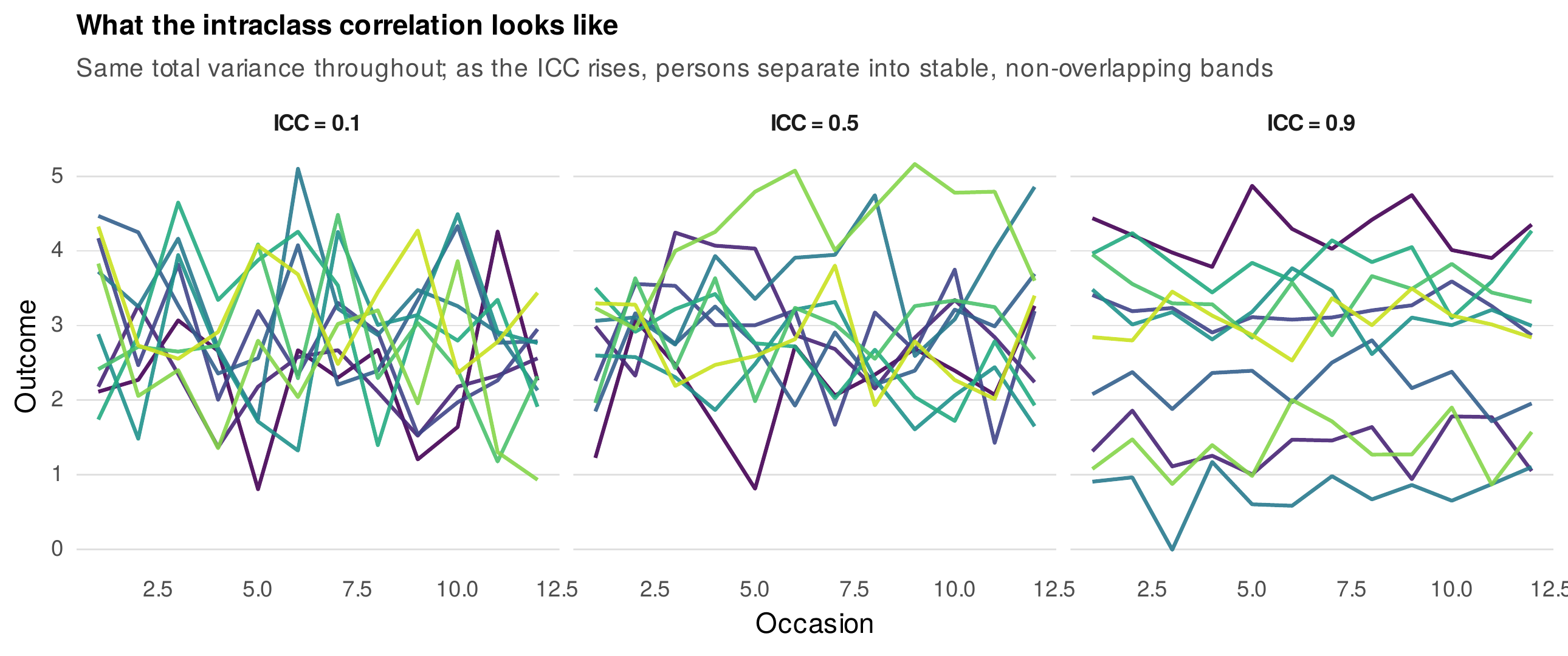
Note. Ten simulated persons, each measured on twelve occasions, with the same total variance in every panel. As the ICC rises from \(0.1\) to \(0.9\), the share of variance that is stable and between persons grows, and the trajectories separate from a tangled band into distinct, persistent levels. The ICC is thus both the proportion of between-person variance and the expected within-person correlation of two observations.
For the book’s experience-sampling data, the null models place momentary negative affect at an ICC of \(0.36\), positive affect at \(0.43\), and momentary stress at \(0.47\), values in the range typically reported for affective and behavioral constructs measured intensively, roughly \(0.3\) to \(0.6\) (Bolger & Laurenceau, 2013). The reading is immediate and consequential: for each of these variables, somewhat more than half of the variance is momentary, which is precisely the within-person variation that experience-sampling designs exist to capture. The contrast with a nearly trait-like variable is instructive: the momentary situational indicator of being alone has an ICC indistinguishable from zero in these data, meaning that whether a person is alone at a given beep is almost entirely a within-person, situational matter with little stable between-person component, a variable whose variance lives where a between-person questionnaire could never reach it. A construct with an ICC near one presents the opposite problem, that within-person questions are starved of variance, and no amount of intensive sampling will manufacture the fluctuation that the construct does not exhibit.
Intensive designs invite a further decomposition, because their occasions are themselves nested, beeps within days within persons, and a three-level null model partitions the variance into person, day, and moment shares. For negative affect the shares are \(0.35\) between persons, \(0.14\) between days within persons, and \(0.51\) within days, so that roughly a seventh of the total variance is day-level, a meaningful amount that describes how day-structured the construct is, whether affect has good days and bad days over and above its moment-to-moment noise. Stress, by contrast, shows a smaller day share (\(0.06\)), suggesting that its fluctuations are more purely momentary than diurnally organized. The final and most important caution is that the ICC is not a fixed property of a construct. It depends on the timescale and the sampling scheme: sampling the same construct hourly, daily, and yearly will yield different decompositions, because the boundary between within and between shifts with the window. An ICC is a statement about a variable in a design, not about a variable in the abstract.
7.2 Decomposing Predictors: Centering as a Descriptive Act
The same partition that describes an outcome also applies to a predictor, and performing it is the descriptive foundation of every within-person model to come. Any time-varying variable can be written as the sum of a person-specific mean and a momentary deviation, \(x_{it} = \bar{x}_{i\cdot} + (x_{it} - \bar{x}_{i\cdot})\), where the person mean \(\bar{x}_{i\cdot}\) is a between-person quantity, a proxy for the person’s trait level, and the deviation \(x_{it} - \bar{x}_{i\cdot}\) is a within-person quantity, the momentary departure from that person’s own baseline. This is not merely a computational convenience but a substantive separation, because the two components can relate to an outcome in different, even opposite, ways, the phenomenon introduced conceptually in Chapter 1 and formalized in the multilevel models of Chapters 13 and 23. Figure 7.2 shows the separation empirically for the association between stress and negative affect in the experience-sampling data. The between-person panel plots person-mean stress against person-mean negative affect, one point per person, and reveals that people who are more stressed on average are also more negative on average, a between-person correlation of \(0.55\). The within-person panel plots each person’s momentary stress deviations against their momentary negative-affect deviations, and its pooled slope, a within-person correlation of \(0.33\), answers a different question: when a given person is more stressed than usual, are they also more negative than usual? Both associations are positive here, but they are not the same number and need not even share a sign, and conflating them is the ecological fallacy that within-person methods exist to prevent.
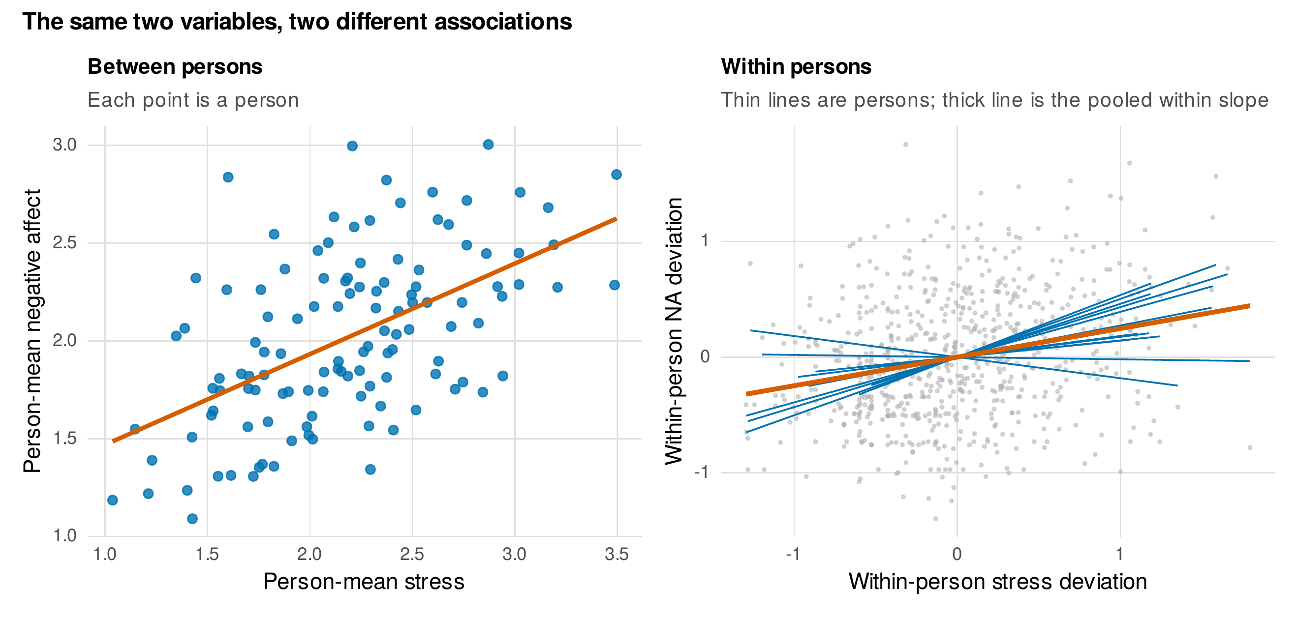
Note. Left: person-mean stress against person-mean negative affect (one point per person), the between-person association (\(r = 0.55\)). Right: within-person stress deviations against within-person negative-affect deviations; thin lines are individual persons and the thick line is the pooled within-person slope (\(r = 0.33\)). The two associations answer different questions and are estimated from different variance.
A caution attaches to the observed decomposition that becomes important when the number of occasions is small. The person mean \(\bar{x}_{i\cdot}\) is not the person’s true trait level but an estimate of it, contaminated by sampling error whose variance is \(\sigma^2/T_i\), so that with few occasions the observed person means are more dispersed than the true trait means and the observed between-person variance is inflated. The consequence is that a decomposition built from raw person means treats each person’s estimated average as if it were known exactly, which it is not. The model-based remedy, developed in Chapter 13, is to replace the raw person mean with a shrinkage estimate that pulls unreliable individual means toward the grand mean in proportion to their uncertainty, and the fully latent decomposition of dynamic structural equation models (Chapter 25) removes the contamination entirely by separating true from error variance at estimation time. For now the descriptive point stands: centering is a decomposition, the decomposition is informative, and its raw form carries a known bias that later chapters correct.
Foundations Box • The within-and-between decomposition, and why small \(T\) bites
Write the person mean as \(\bar{x}_{i\cdot} = \frac{1}{T_i}\sum_t x_{it}\) and decompose \(x_{it} = \bar{x}_{i\cdot} + \tilde{x}_{it}\) with \(\tilde{x}_{it} = x_{it} - \bar{x}_{i\cdot}\). By construction \(\sum_t \tilde{x}_{it} = 0\) within each person, so the within component is orthogonal to the between component, and the total variance decomposes additively, \(\mathrm{Var}(x_{it}) \approx \mathrm{Var}(\bar{x}_{i\cdot}) + \mathrm{Var}(\tilde{x}_{it})\). If each person has a true trait level \(\mu_i\) with \(x_{it} = \mu_i + \varepsilon_{it}\) and \(\mathrm{Var}(\varepsilon_{it}) = \sigma^2\), then \(E[\bar{x}_{i\cdot}] = \mu_i\) but \(\mathrm{Var}(\bar{x}_{i\cdot} \mid \mu_i) = \sigma^2 / T_i\). The observed spread of person means therefore exceeds the true trait variance by an amount \(\sigma^2 / T_i\), which vanishes only as \(T_i\) grows. This is why person means computed from short series are noisy trait estimates, why observed between-person variance is upward biased at small \(T\), and why shrinkage (Chapter 13) and latent decomposition (Chapter 25) improve on the raw calculation.
7.3 A Catalogue of Intraindividual Dynamics Indices
Once the data are viewed within persons, each individual’s series can be summarized by indices that target distinct features of the process, and these indices serve a dual role: as descriptive summaries now and, in later chapters, as outcomes or predictors in their own right. The guiding pedagogy is index now, model later, because each descriptive index has a model-based analogue that estimates the same quantity with proper uncertainty, the mixed-effects location-scale model for within-person variability (Chapter 16) and the multilevel autoregressive model for inertia (Chapter 25). Figure 7.3 is the chapter’s signature teaching figure, and it makes the case for the whole enterprise: four people with identical means but strikingly different dynamics. The stable person varies little; the volatile person swings widely and rapidly; the drifting person also varies widely but slowly, so that although the drifting person’s within-person standard deviation (\(0.78\)) exceeds the volatile person’s (\(0.67\)), its successive differences are far smaller because change is gradual rather than abrupt; and the bursty person is usually calm but punctuated by occasional acute jumps. A single summary, the mean, is blind to all of this, and even a single variability index would confuse the volatile and drifting persons. Capturing the difference requires several indices, each defined below with the feature it targets and the caution it demands, and collected in Table 7.1.
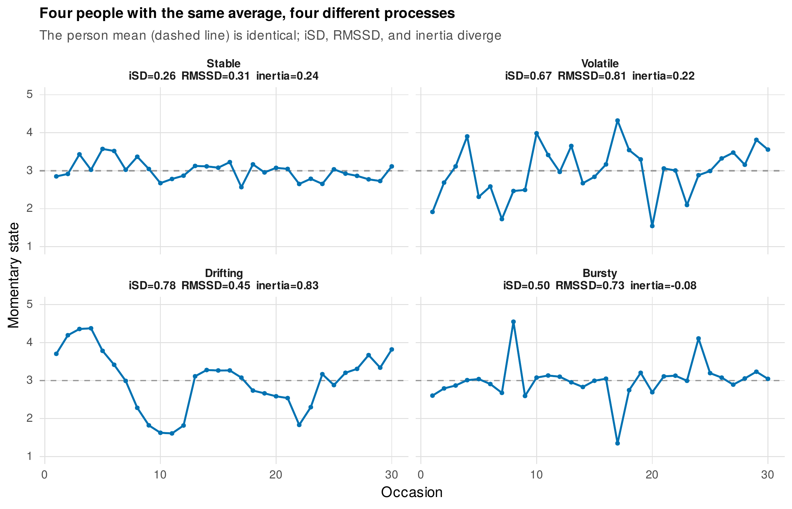
Note. Each panel is one simulated person measured on thirty occasions; the dashed line marks the common person mean, which is identical across panels. The within-person standard deviation (iSD), the root mean square of successive differences (RMSSD), and lag-1 inertia diverge sharply. Note that the drifting person has a larger iSD than the volatile person but a much smaller RMSSD, because slow change produces small successive differences.
Location is summarized by the intraindividual mean (iMean), the person’s average level, which for many purposes is the single most predictive index and against which every variability measure must be checked. Variability is summarized by the intraindividual standard deviation (iSD), the standard deviation of a person’s own observations, which quantifies how widely the state ranges but which, on a bounded scale, is mechanically entangled with the mean in a way addressed in the next section and corrected by the relative standard deviation (Mestdagh et al., 2018). Instability, the tendency to change abruptly from one moment to the next, is summarized by the root mean square of successive differences (RMSSD), \(\sqrt{\frac{1}{T-1}\sum_{t=2}^{T}(x_t - x_{t-1})^2}\), which unlike the iSD is sensitive to the temporal ordering of the observations and so distinguishes rapid oscillation from slow drift (Jahng et al., 2008); a related instability index is the probability of acute change (PAC), the proportion of successive transitions that exceed a chosen threshold, which isolates the frequency of large jumps. Inertia, the tendency of a state to persist, is summarized by the person-level lag-1 autocorrelation, the correlation of each observation with the preceding one, which has been linked to emotional regulation and, when elevated, to maladjustment (Kuppens et al., 2010); it is the descriptive precursor of the autoregressive parameter of Chapter 24, and it carries a serious small-sample caution developed below. Cross-construct dynamics are summarized by within-person correlations between two states, and, for sets of emotion items, by emotion differentiation, operationalized as the average within-person correlation among same-valence items, where a low average correlation indicates a person who distinguishes finely among their negative states and a high one a person for whom all negative feelings move together (Erbas et al., 2014); in the item-level experience-sampling data the mean within-person correlation among the four negative-affect items is \(0.27\), indicating moderate differentiation on average.
Table 7.1. A catalogue of intraindividual dynamics indices.
| Index | Feature targeted | Computation | Main caution |
|---|---|---|---|
| iMean | Average level | Mean of the person’s observations | Often the strongest predictor; control it before crediting other indices |
| iSD | Overall variability | SD of the person’s observations | Confounded with the mean on bounded scales |
| Relative SD | Mean-corrected variability | iSD divided by its maximum given the mean and bounds | Undefined near the scale limits |
| RMSSD | Instability / abruptness | Root mean of squared successive differences | Sensitive to ordering; inflated by trends and cycles |
| PAC | Frequency of large jumps | Proportion of \(|\)successive difference\(|\) above a cutoff | Cutoff choice is arbitrary; report it |
| Inertia | Persistence / carryover | Person-level lag-1 autocorrelation | Severely downward biased at small \(T\) |
| Within-person \(r\) | Coupling of two states | Correlation of momentary deviations | Requires enough occasions per person |
| Differentiation | Granularity of states | Mean within-person correlation among same-valence items | Confounded with variability and mean |
Note. Each index has a model-based analogue that estimates the same feature with shrinkage and proper uncertainty: the mixed-effects location-scale model for variability (Chapter 16) and the multilevel autoregressive model for inertia (Chapter 25). Compute the index to describe; fit the model to infer.
A complementary framing, due to Fleeson (2001), resists reducing the within-person series to any single index and instead treats the whole within-person distribution as the object of interest, the density-distribution view in which a trait is the density of the states a person visits over time. Figure 7.4 realizes this view for twelve persons, ordered by their mean level of momentary negative affect, and it recovers by eye what the indices quantify: persons low in average negative affect show right-skewed distributions bunched against the floor of the scale, while higher persons show broader, more symmetric distributions, so that mean, spread, and shape covary in ways a single number cannot convey. The density view is a useful antidote to index proliferation, a reminder that the indices are lossy summaries of a richer object.
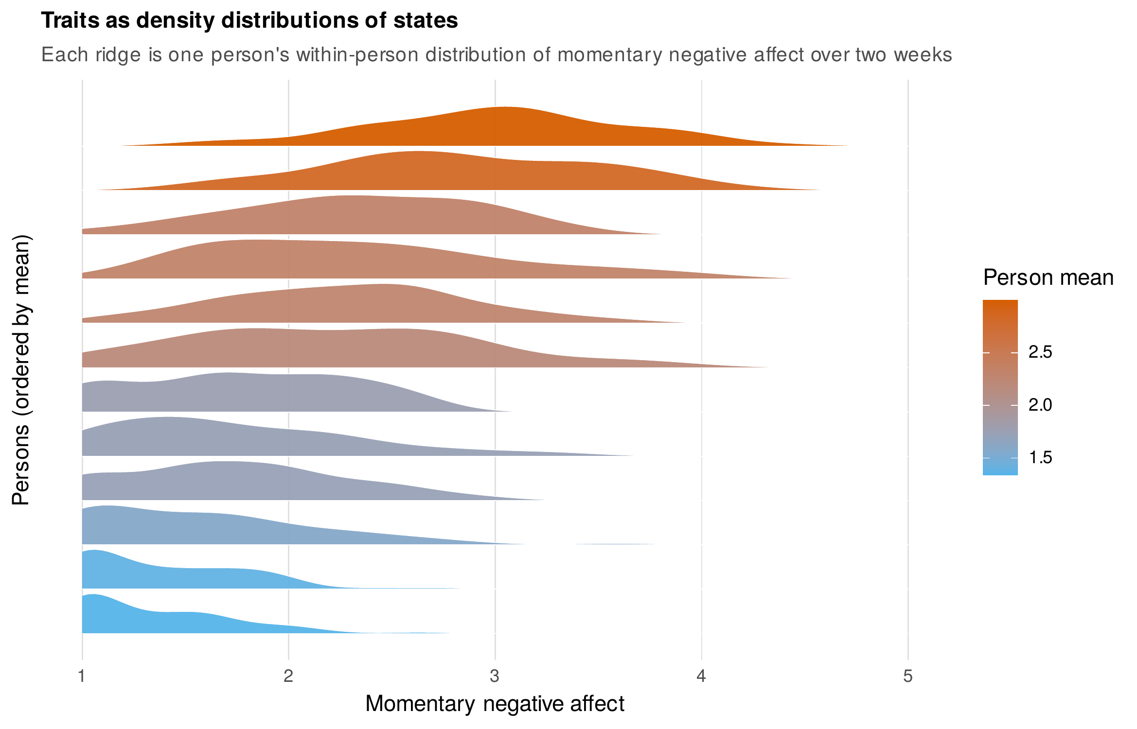
Note. Each ridge is one person’s within-person distribution of momentary negative affect across two weeks of sampling, with persons ordered and shaded by their mean level. Low-mean persons show right-skewed distributions pressed against the scale floor; higher-mean persons show broader, more symmetric distributions. The whole distribution, not just its mean or SD, is the descriptive object in Fleeson’s framing.
7.4 How Trustworthy Are the Indices?
The catalogue would be dangerous without its counterweight, because person-level indices are estimated from finite series and inherit all the frailties of small samples, and three problems in particular can turn an index into an artifact. The first is the mean-variance confound. On a bounded scale, the variance a person can exhibit is limited by how close their mean sits to the scale’s floor or ceiling: a person averaging near the minimum has little room to vary, while a person near the scale’s midpoint can range widely, so that the iSD is mechanically tied to the iMean even when the underlying process is identical. Figure 7.5 demonstrates the problem and its correction in the experience-sampling data. The left panel plots each person’s iSD against their iMean, with the parabolic envelope showing the maximum standard deviation attainable at each mean on a one-to-five scale; the observed points hug the floor region and correlate \(0.61\) with the mean, so that a naive analysis relating variability to an outcome would in part be relating the mean to the outcome. The relative standard deviation of Mestdagh et al. (2018) removes the artifact by expressing each person’s iSD as a fraction of the maximum it could have taken given their mean, and the right panel shows that after this correction the association with the mean is no longer positive. The practical rule follows directly: on bounded scales, never interpret a raw iSD without either controlling for the mean or replacing it with a mean-corrected index, because otherwise a finding about variability may be a finding about level in disguise.
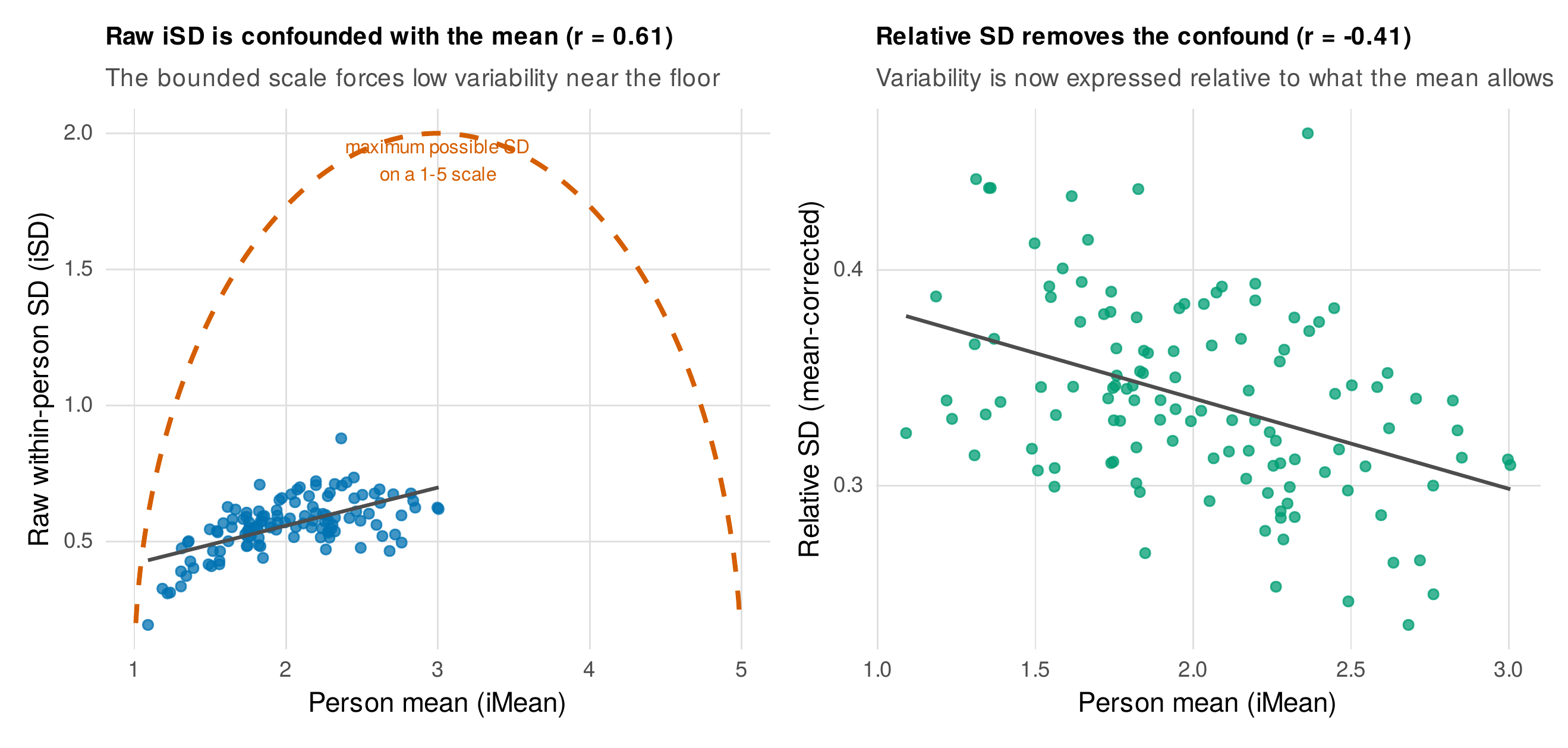
Note. Left: raw within-person SD against the person mean; the dashed parabola is the maximum SD attainable at each mean on a bounded one-to-five scale, and the observed correlation is \(0.61\). Right: the relative SD, which divides the observed SD by that maximum, is no longer positively confounded with the mean (\(r = -0.41\)). Any conclusion about variability drawn from the raw iSD must be checked against this confound.
The second problem is reliability, the question of how many occasions an index needs before it estimates a stable person characteristic rather than noise. Because an index is computed from a person’s series, its reliability grows with the length of that series, and different indices grow at very different rates. Figure 7.6 reports a split-half reliability simulation, in which each index is computed on two independent halves of a person’s data and correlated across persons, as a function of the number of occasions. The variability indices are relatively well behaved: the iSD and RMSSD reach a reliability near \(0.80\) by about thirty occasions and exceed \(0.94\) by one hundred. Inertia is far more demanding: the lag-1 autocorrelation attains a reliability of only \(0.11\) at ten occasions and \(0.36\) at thirty, and does not approach acceptable levels until the series is very long, because estimating a correlation over time requires many transitions. The lesson is that inertia should be treated as an unreliable person-level index in the short series typical of daily-diary studies, and that its model-based estimation with shrinkage (Chapter 25), which borrows strength across persons, is not a refinement but a necessity.
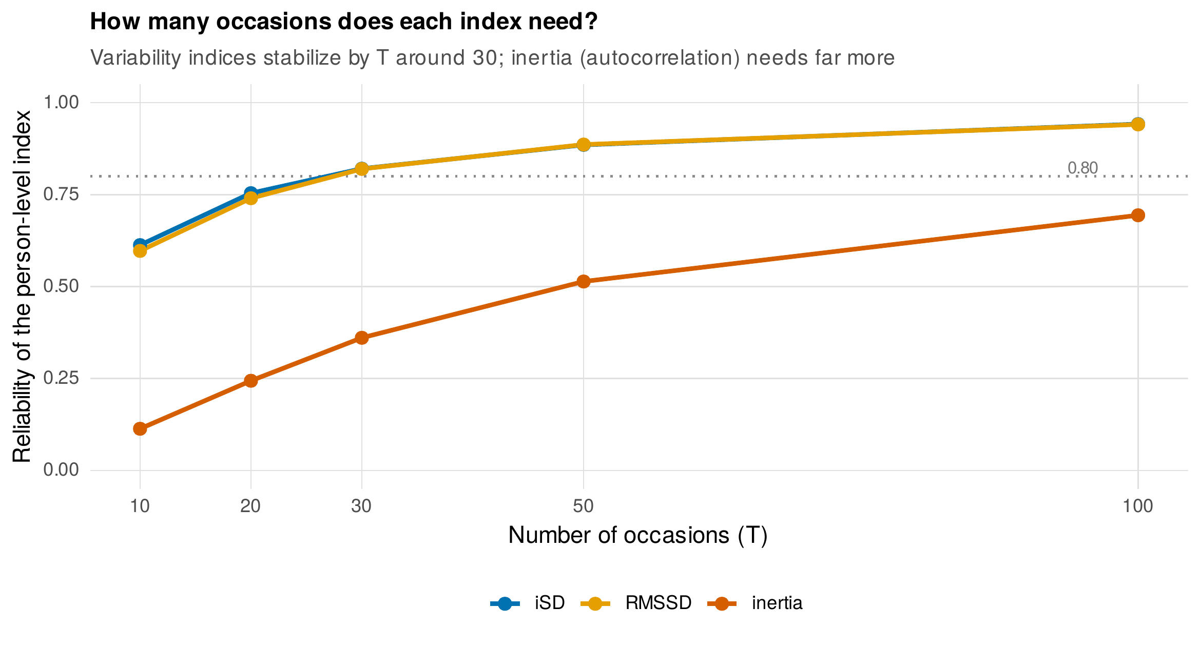
Note. Split-half reliability of three indices against the number of occasions \(T\), from a simulation with between-person variation in mean, variability, and inertia. The variability indices (iSD, RMSSD) cross the conventional \(0.80\) threshold near \(T = 30\); inertia, the lag-1 autocorrelation, remains unreliable well beyond that and needs a much longer series or model-based estimation.
Inertia’s difficulty has a second face beyond low reliability, a systematic small-sample bias: the sample autocorrelation is biased downward in short series, so that even its average understates the true persistence. In a simulation with a true lag-1 autocorrelation of \(0.40\), the sample estimate averages only \(0.17\) at ten occasions, \(0.33\) at thirty, and does not close to within a rounding error of the truth until one hundred occasions. The bias is of order \(1/T\) and is a classical result for the autoregressive model (the leading-order correction is approximately \(-(1 + 3\varphi)/T\)), and its practical implication is severe: comparisons of inertia across persons or groups measured with different series lengths are confounded by differential bias, and a group with shorter records will appear less inertial than it is. The Foundations box below states the two biases together. The third problem is contamination by systematic trends, because both variability and instability indices assume that the within-person fluctuations are the signal, when a portion of them may be a predictable trend or cycle. Figure 7.7 makes the point with a diurnal rhythm: a series that rises and falls with the time of day exhibits an RMSSD of \(0.65\), but once the daily cycle is modeled and removed, the RMSSD of the residuals falls to \(0.28\), so that more than half of the apparent instability was in fact a predictable rhythm counted as noise. Whether to remove such structure is a decision, not a default, and Table 7.2 offers a decision guide; the governing question is whether the trend or cycle is part of the process one wishes to describe or a nuisance to be partialled out before describing the residual dynamics.
Foundations Box • Two biases in the lag-1 autocorrelation
The sample lag-1 autocorrelation \(r_1 = \sum_{t=2}^{T}(x_t - \bar{x})(x_{t-1} - \bar{x}) / \sum_{t=1}^{T}(x_t - \bar{x})^2\) suffers two distinct small-\(T\) problems. First, it is negatively biased: for an AR(1) process with parameter \(\varphi\), the expectation is approximately \(E[r_1] \approx \varphi - (1 + 3\varphi)/T\), so short series systematically understate persistence, and the bias differs across series of different length. Second, it is unreliable: its sampling variance is large at small \(T\), so two halves of the same person’s data yield weakly correlated estimates (Figure 7.6). The two problems compound, and both are why person-level inertia computed from daily-diary-length series is treated with caution and why the multilevel autoregressive models of Chapter 25, which pool information across persons and separate measurement error from dynamics, are the proper estimation tool.
Table 7.2. A detrending decision guide for variability and instability indices.
| If the research question concerns … | Then handle systematic structure by … |
|---|---|
| Total within-person variability, cycles included | Computing indices on the raw series; report that trends are retained |
| Dynamics net of predictable rhythms | Removing linear trend and diurnal cycle first; compute indices on residuals |
| The diurnal cycle itself | Modeling the cycle explicitly (Chapters 23, 30); the cycle is the signal |
| Comparing persons with different trends | Detrending per person, or modeling trend and dynamics jointly, to avoid confounding |
Note. Detrending is a substantive choice, not a technical default. Removing a cycle answers a different question from retaining it, and the two can give opposite conclusions about who is most unstable. State the choice and its rationale.
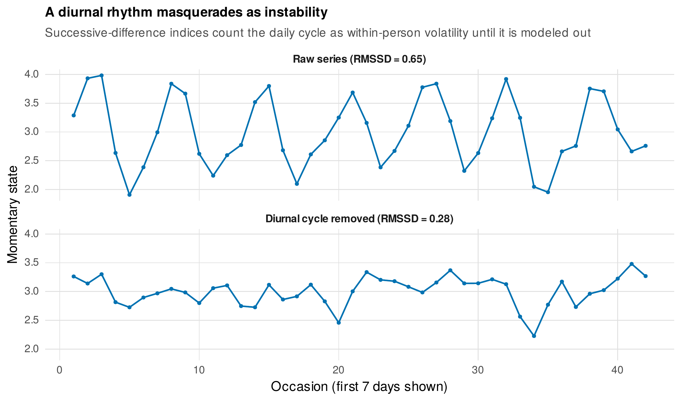
Note. Top: a simulated momentary series with a diurnal cycle has an RMSSD of \(0.65\). Bottom: after the daily cycle is modeled and removed, the residual RMSSD falls to \(0.28\). More than half of the apparent moment-to-moment instability was a predictable rhythm. Whether to remove it depends on the research question (Table 7.2).
Finally, even indices that are individually trustworthy may be collectively redundant, measuring so nearly the same thing that entering several of them into a model buys nothing but multicollinearity, and adds little beyond the mean for predicting outcomes (Dejonckheere et al., 2019). Figure 7.8 displays the empirical correlations among the person-level indices in the experience-sampling data, and the pattern is sobering: RMSSD and PAC correlate \(0.88\), being two views of the same instability; the iMean bleeds into the iSD at \(0.61\), the confound documented above; and only the relative SD and inertia stand meaningfully apart from the variability cluster. The implication is not that the indices are useless but that they must be chosen deliberately, one representative per feature, rather than accumulated, and that any incremental claim, that a dynamics index predicts an outcome over and above the mean, must be tested against the mean and against the other indices rather than asserted.
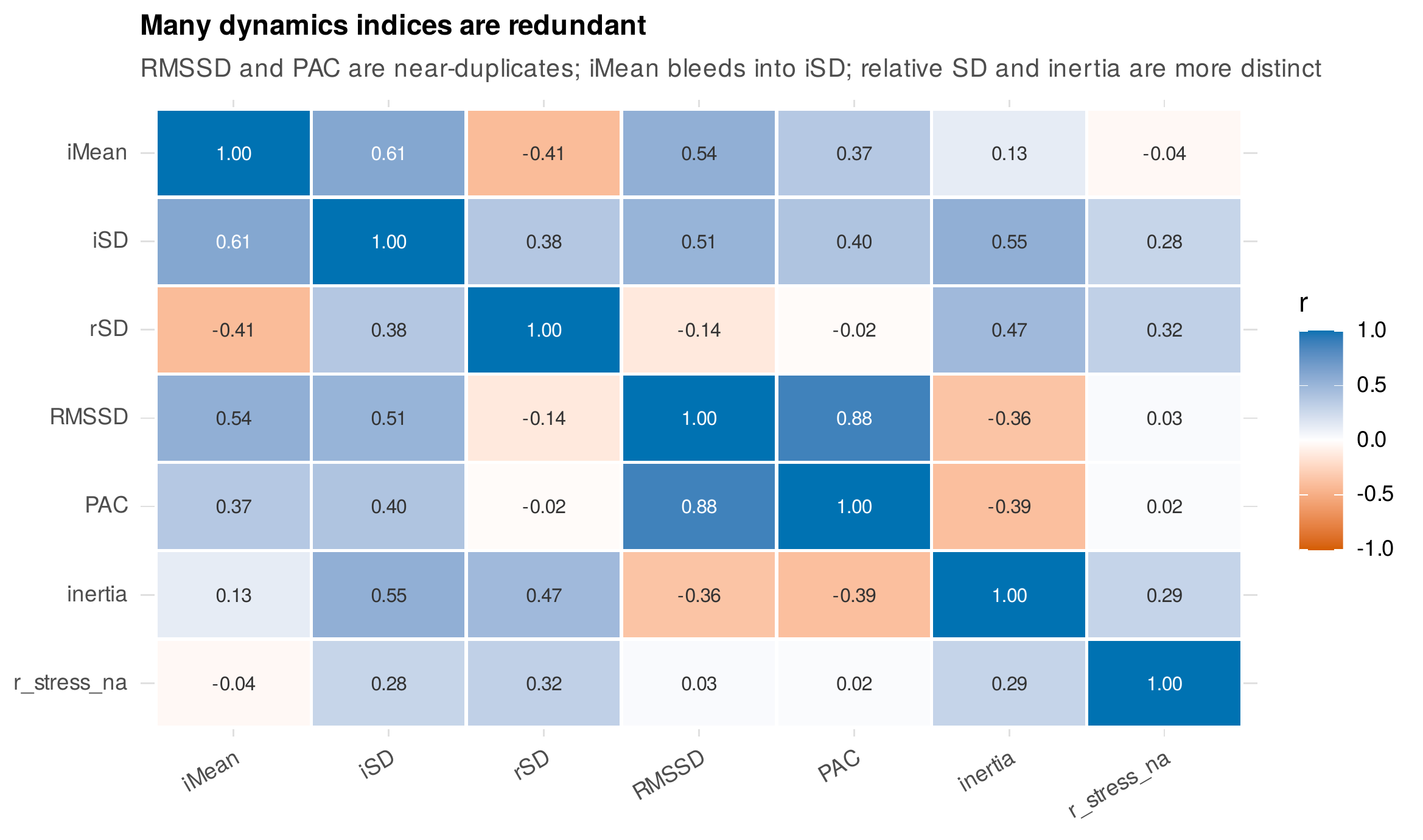
Note. Empirical correlations among the person-level indices in the experience-sampling data. RMSSD and PAC (\(0.88\)) are near-duplicates; the mean bleeds into the iSD (\(0.61\)). Only the relative SD and inertia are substantially distinct from the variability cluster. Entering several redundant indices together produces multicollinearity, not insight.
Common Pitfall • three ways an index misleads
First, crediting variability without controlling the mean: because iSD is confounded with iMean on bounded scales (Figure 7.5), a correlation between iSD and an outcome may be the mean’s correlation in disguise; always control the mean or use the relative SD. Second, computing instability or inertia on a trended series: RMSSD and the autocorrelation absorb any diurnal cycle or linear trend as if it were within-person noise (Figure 7.7), so decide explicitly whether to detrend. Third, comparing iSD across scales with different bounds: because the mean-variance confound depends on the scale limits, an iSD of \(0.7\) on a one-to-five scale is not comparable to \(0.7\) on a one-to-seven scale; compare relative variability, not raw SDs, across instruments.
7.5 Descriptive Tables for Repeated Measures
The descriptive apparatus of this chapter culminates in the longitudinal Table 1, the level-aware descriptive table that every intensive or panel study should report and that a reader needs in order to judge the analyses that follow. It differs from a cross-sectional Table 1 in reporting level-specific information: not one mean and standard deviation per variable but the decomposition of variance across levels, and not one correlation matrix but two, because between-person and within-person associations differ. Table 7.3 is a model descriptive table for the experience-sampling data. Each variable carries its grand mean, its total standard deviation, and its person-level and day-level intraclass correlations, and the correlation matrix reports between-person correlations above the diagonal and within-person correlations below it. The two triangles tell different stories, as the decomposition of Section 7.2 predicts: negative and positive affect correlate \(-0.50\) between persons but only \(-0.32\) within persons, and stress and positive affect correlate \(-0.52\) between persons yet a negligible \(-0.11\) within, so that the trait-level opposition of stress and positive mood is far stronger than their moment-to-moment coupling. A single, undifferentiated correlation would have obscured this. The software note records the several packages that automate parts of this table, with the warning that their intraclass-correlation definitions do not always agree.
Table 7.3. Model descriptive table for the experience-sampling data.
| Variable | \(M\) | \(SD\) | \(\mathrm{ICC}_{p}\) | \(\mathrm{ICC}_{d}\) | 1 | 2 | 3 |
|---|---|---|---|---|---|---|---|
| 1. Negative affect | 2.01 | 0.71 | .35 | .14 | – | \(-.50\) | \(.55\) |
| 2. Positive affect | 3.22 | 0.82 | .43 | .10 | \(-.32\) | – | \(-.52\) |
| 3. Stress | 2.16 | 0.74 | .47 | .06 | \(.33\) | \(-.11\) | – |
Note. \(M\) and \(SD\) are computed over all person-occasions. \(\mathrm{ICC}_{p}\) and \(\mathrm{ICC}_{d}\) are the person-level and day-level intraclass correlations from a three-level null model. Correlations above the diagonal are between persons (person means); correlations below the diagonal are within persons (person-centered deviations). \(N = 120\) persons, up to \(84\) occasions each.
7.6 Running the Descriptives in R
The worked example computes every quantity in this chapter for the experience-sampling data. The intraclass correlations come from null multilevel models, whose variance components are read directly and combined; the two-level version gives the person ICC and the three-level version adds the day share.
library(lme4); library(dplyr); library(tidyr)
ae <- readRDS("Examples/data/affect_ema.rds")

# --- ICC from a two-level null model ---
m2  <- lmer(na ~ 1 + (1 | person), data = ae)
vc  <- as.data.frame(VarCorr(m2))
tau <- vc$vcov[vc$grp == "person"]; sig <- vc$vcov[vc$grp == "Residual"]
icc_person <- tau / (tau + sig)                 # 0.36 for negative affect

# --- Three-level variance shares: beeps in days in persons ---
m3  <- lmer(na ~ 1 + (1 | person/day), data = ae)   # person and day:person
vc3 <- as.data.frame(VarCorr(m3))
shares <- vc3$vcov / sum(vc3$vcov)              # person, day, moment shares
The person-level indices are computed with a single documented function applied to each person’s ordered series. The shipped script defines the function compute_dynamics_indices(), applies it by person, and goes on to compute the redundancy matrix, the reliability simulation, and the small-sample autocorrelation bias reported above.
# compute_dynamics_indices(): iMean, iSD, relative SD, RMSSD, PAC, inertia
compute_dynamics_indices <- function(x, lo = 1, hi = 5, pac_cut = 1) {
  xo <- x[!is.na(x)]; if (length(xo) < 3) return(rep(NA, 6))
  m <- mean(xo); s <- sd(xo)
  maxsd <- sqrt((hi - m) * (m - lo))            # max SD at this mean on [lo,hi]
  rSD <- if (maxsd > 0) s / maxsd else NA       # Mestdagh et al. (2018)
  d <- diff(x); d <- d[!is.na(d)]
  RMSSD <- sqrt(mean(d^2)); PAC <- mean(abs(d) > pac_cut)
  x1 <- x[-length(x)]; x2 <- x[-1]; ok <- !is.na(x1) & !is.na(x2)
  inertia <- if (sum(ok) >= 3) cor(x1[ok], x2[ok]) else NA
  c(iMean = m, iSD = s, rSD = rSD, RMSSD = RMSSD, PAC = PAC, inertia = inertia)
}

person_idx <- ae %>% arrange(person, day, beep) %>% group_by(person) %>%
  summarise(as.data.frame(t(compute_dynamics_indices(na))), .groups = "drop")

cor(person_idx[, -1], use = "pairwise.complete.obs")   # redundancy matrix
The descriptive Table 1 assembles the level-specific statistics and the two correlation matrices. The between-person correlations are computed from person means, and the within-person correlations from person-centered deviations, exactly the decomposition of Section 7.2 applied to every pair.
pm  <- ae %>% group_by(person) %>%
  summarise(across(c(na, pa, stress), ~mean(.x, na.rm = TRUE)))
between_cor <- cor(pm[, -1], use = "complete.obs")     # above the diagonal
aew <- ae %>% group_by(person) %>%
  mutate(across(c(na, pa, stress), ~ .x - mean(.x, na.rm = TRUE), .names = "wd_{.col}"))
within_cor <- cor(aew[, c("wd_na","wd_pa","wd_stress")], use = "pairwise.complete.obs")
Software Note • descriptive helpers, and a warning about ICC definitions
Several packages automate parts of the longitudinal Table 1: psych::statsBy returns between- and within-person correlations and reliabilities in one call; misty::multilevel.descript reports level-specific descriptives and intraclass correlations; and performance::icc extracts the ICC from a fitted model. The essential caution is that the term “ICC” names a family, not a single quantity: packages differ in whether they report the unadjusted or adjusted ICC, the one-way or two-way form, and, for three-level data, which level’s share, so a reported ICC should always be accompanied by the model and definition that produced it. Computing the ICC from an explicit null model, as above, makes the definition unambiguous.
7.7 Interpreting and Reporting Descriptive Results
A descriptive section for an intensive study should report where the variance lies, how the indices behave, and the level-specific associations, in language that keeps the levels distinct. A model paragraph for the experience-sampling data reads: “Momentary negative affect, positive affect, and stress showed person-level intraclass correlations of \(.35\), \(.43\), and \(.47\) respectively (three-level null models), indicating that roughly half of the variance in each was momentary and available to within-person analysis; a further \(6\) to \(14\%\) was organized at the day level. Person means and person-centered deviations were computed for each variable. The between-person and within-person association of stress with negative affect differed in magnitude (\(r = .55\) and \(r = .33\)), consistent with distinct trait-level and state-level processes. Within-person variability was summarized by the relative standard deviation rather than the raw within-person standard deviation, because the latter correlated \(.61\) with the person mean on the bounded response scale. Lag-1 inertia was computed but is reported with caution, as its reliability at the achieved number of occasions is low.” Every clause reports a level-specific quantity and flags the one index, inertia, whose trustworthiness the data cannot support, which is precisely the honesty this chapter is designed to instill.
7.8 Common Misconceptions
Several beliefs about these descriptives mislead. The first equates the intraclass correlation with reliability; the two are computed from similar variance ratios and are related, but the ICC of an outcome describes how much of its variance is between persons, whereas the reliability of a measure describes how much of its variance is true score, and a variable can have a low ICC while being measured perfectly. The second holds that high inertia is always maladaptive; the empirical literature links elevated inertia to poorer adjustment on average, but persistence is adaptive or maladaptive depending on what is persisting and in what context, and moralizing an index is a conceptual error. The third treats person means as the person’s true levels; they are estimates contaminated by sampling error that is substantial when occasions are few, and the shrinkage and latent-decomposition methods of later chapters exist because the raw mean overstates between-person dispersion. A recurring question, which variability index to use, is answered by Table 7.1’s logic of matching the index to the process feature of interest, tempered by the redundancy warning: choose one representative of each feature rather than reporting a correlated battery, and on bounded scales prefer the mean-corrected form.
In Practice • minimum occasions per index
The number of occasions an index needs is not one number but depends on the index and on the reliability one is willing to accept. In the simulation of Figure 7.6, the within-person mean and standard deviation reach a split-half reliability near \(.80\) by roughly thirty occasions, and the RMSSD is similar. Lag-1 inertia is far more demanding, remaining below \(.40\) at thirty occasions and requiring a much longer series, or model-based estimation that borrows strength across persons, before a person-level value can be trusted. These figures are specific to the simulated process and should be read as order-of-magnitude guidance, not as thresholds: the honest practice is to report the achieved number of occasions and to treat person-level indices computed from short series, especially autocorrelation-based ones, as provisional.
Chapter Summary
Descriptive analysis of repeated measures begins by asking where the variance lives. The intraclass correlation from a null model partitions total variance into between-person and within-person shares and doubles as the expected within-person correlation (Figure 7.1); for the book’s affect data roughly half of the variance in each momentary construct is within persons, with a further tenth at the day level. Any time-varying predictor decomposes into a between-person mean and a within-person deviation, whose associations with an outcome can differ (Figure 7.2), and the raw person mean is a noisy trait estimate at small \(T\). A family of person-level indices summarizes each individual’s dynamics, the mean, the standard deviation and its mean-corrected relative form, the RMSSD and probability of acute change for instability, and the lag-1 autocorrelation for inertia, and four people with identical means can differ sharply on them (Figure 7.3). Every index carries a failure mode: the raw iSD is confounded with the mean on bounded scales and must be corrected (Figure 7.5); inertia is both unreliable and downward biased in short series (Figure 7.6); trends and diurnal cycles inflate instability unless modeled out (Figure 7.7); and the indices are mutually redundant, adding little beyond the mean (Figure 7.8). The chapter closes with the longitudinal Table 1, which reports level-specific statistics and separate between- and within-person correlation matrices. Throughout, the discipline is to compute an index to describe and to fit a model to infer.
Where to Go Next
The descriptives of this chapter are the entry point to the modeling parts. The variance decomposition is the null model that every multilevel growth and diary model (Chapters 13, 14, 23) elaborates, and the ICC it yields determines how much within-person signal those models have to work with. The between-and-within decomposition of a predictor becomes the centering decision at the heart of within-person modeling. The variability indices become model parameters in the mixed-effects location-scale models of Chapter 16, and inertia becomes the autoregressive parameter of the single-subject and multilevel time-series models of Chapters 24 and 25, estimated there with the shrinkage and error separation that the descriptive indices lack. In the applications of Chapters 33 and 35 these indices reappear as predictors of clinical and personality outcomes, where the cautions rehearsed here, the mean confound, the reliability floor, the redundancy, are the difference between a robust finding and an artifact.
Exercises
- 7.1 Decompose the variance. Compute two-level and three-level intraclass correlations for five variables in
affect_ema, at the person and day levels. Interpret what each value implies for whether the construct is better studied within or between persons. - 7.2 Two associations. Build the between-person and within-person decomposition scatterplots for stress and negative affect, estimate both slopes, and write a \(150\)-word interpretation that keeps the two levels distinct and names the fallacy that conflating them would commit.
- 7.3 Expose the confound. Reproduce the mean-iSD scatter with its bounded-scale envelope, then apply the relative standard deviation, and report how a hypothetical correlation between variability and an outcome would change once the mean confound is removed.
- 7.4 Bias of inertia. By simulation, estimate the bias of the lag-1 autocorrelation at \(T = 10\), \(30\), and \(100\) for a true value of your choosing, and state the consequence for comparing inertia across studies with different series lengths.
- 7.5 Build Table 1. Using a provided diary dataset and the template of Table 7.3, produce a publication-grade descriptive table with level-specific statistics and separate between- and within-person correlation matrices, and write the accompanying descriptive paragraph.
References
Baird, B. M., Le, K., & Lucas, R. E. (2006). On the nature of intraindividual personality variability: Reliability, validity, and associations with well-being. Journal of Personality and Social Psychology, 90(3), 512–527. https://doi.org/10.1037/0022-3514.90.3.512
Bliese, P. D. (2000). Within-group agreement, non-independence, and reliability: Implications for data aggregation and analysis. In K. J. Klein & S. W. J. Kozlowski (Eds.), Multilevel theory, research, and methods in organizations: Foundations, extensions, and new directions (pp. 349–381). Jossey-Bass.
Bolger, N., & Laurenceau, J.-P. (2013). Intensive longitudinal methods: An introduction to diary and experience sampling research. Guilford Press.
Dejonckheere, E., Mestdagh, M., Houben, M., Rutten, I., Sels, L., Kuppens, P., & Tuerlinckx, F. (2019). Complex affect dynamics add limited information to the prediction of psychological well-being. Nature Human Behaviour, 3(5), 478–491. https://doi.org/10.1038/s41562-019-0555-0
Enders, C. K., & Tofighi, D. (2007). Centering predictor variables in cross-sectional multilevel models: A new look at an old issue. Psychological Methods, 12(2), 121–138. https://doi.org/10.1037/1082-989X.12.2.121
Erbas, Y., Ceulemans, E., Pe, M. L., Koval, P., & Kuppens, P. (2014). Negative emotion differentiation: Its personality and well-being correlates and a comparison of different assessment methods. Cognition and Emotion, 28(7), 1196–1213. https://doi.org/10.1080/02699931.2013.875890
Fleeson, W. (2001). Toward a structure- and process-integrated view of personality: Traits as density distributions of states. Journal of Personality and Social Psychology, 80(6), 1011–1027. https://doi.org/10.1037/0022-3514.80.6.1011
Hamaker, E. L. (2012). Why researchers should think “within-person”: A paradigmatic rationale. In M. R. Mehl & T. S. Conner (Eds.), Handbook of research methods for studying daily life (pp. 43–61). Guilford Press.
Houben, M., Van Den Noortgate, W., & Kuppens, P. (2015). The relation between short-term emotion dynamics and psychological well-being: A meta-analysis. Psychological Bulletin, 141(4), 901–930. https://doi.org/10.1037/a0038822
Jahng, S., Wood, P. K., & Trull, T. J. (2008). Analysis of affective instability in ecological momentary assessment: Indices using successive difference and group comparison via multilevel modeling. Psychological Methods, 13(4), 354–375. https://doi.org/10.1037/a0014173
Kuppens, P., Allen, N. B., & Sheeber, L. B. (2010). Emotional inertia and psychological maladjustment. Psychological Science, 21(7), 984–991. https://doi.org/10.1177/0956797610372634
Mestdagh, M., Pe, M. L., Pestman, W., Verdonck, S., Kuppens, P., & Tuerlinckx, F. (2018). Sidelining the mean: The relative variability index as a generic mean-corrected variability measure for bounded variables. Psychological Methods, 23(4), 690–707. https://doi.org/10.1037/met0000153
Shrout, P. E., & Fleiss, J. L. (1979). Intraclass correlations: Uses in assessing rater reliability. Psychological Bulletin, 86(2), 420–428. https://doi.org/10.1037/0033-2909.86.2.420
Trull, T. J., Solhan, M. B., Tragesser, S. L., Jahng, S., Wood, P. K., Piasecki, T. M., & Watson, D. (2008). Affective instability: Measuring a core feature of borderline personality disorder with ecological momentary assessment. Journal of Abnormal Psychology, 117(3), 647–661. https://doi.org/10.1037/a0012532
Wang, L. P., Hamaker, E. L., & Bergeman, C. S. (2012). Investigating inter-individual differences in short-term intra-individual variability. Psychological Methods, 17(4), 567–581. https://doi.org/10.1037/a0029317