Chapter 10
Analyzing Two Occasions: Paired Comparisons, Change Scores, and Reliable Change
Two-occasion data, a measurement before and a measurement after, are the most common longitudinal design and the most often mishandled. This chapter takes them seriously rather than dismissing them as a degenerate case, because the choices they force are the reader’s first encounter with the argument that runs through the rest of the book: the model encodes the question, and two defensible analyses of the same data can reach opposite conclusions because they answer different questions. The chapter builds the paired comparison from first principles, works through the central controversy of change scores versus analysis of covariance and the paradox that dramatizes it, and then turns to two questions that group-level tests cannot answer, whether a particular person changed reliably and whether a group is stable rather than merely not significantly different. It also fixes the template that every methods chapter to come will follow: model, assumptions, estimation, effect size, worked example, and reporting.
Learning Objectives
After working through this chapter, you should be able to: (1) choose and justify the paired \(t\) test, the Wilcoxon signed-rank test, or McNemar’s test from the scale and question; (2) derive the paired \(t\) as a one-sample test on difference scores and explain how the pre-post correlation drives its power; (3) articulate the distinction between change-score and analysis-of-covariance analyses, reproduce Lord’s paradox, and select an analysis by design; (4) compute and interpret paired effect sizes, distinguishing the difference-metric \(d_z\) from the raw-metric \(d_{av}\); (5) apply the reliable change index to classify individual change; (6) test for equivalence when the claim is that no meaningful change occurred; and (7) report a two-occasion analysis to publication standard.
10.1 One Group, Two Occasions
The paired comparison begins by recognizing that a before-and-after measurement on the same person yields not two independent numbers but one difference score, and that reducing each person to their change removes the between-person variation that would otherwise obscure it. The paired \(t\) test is then nothing more than a one-sample \(t\) test asking whether the mean difference departs from zero, and its power advantage over an independent-groups comparison comes entirely from that removal, as the Foundations box derives. The assumption it makes is mild: not that the outcome is normally distributed, but that the differences are approximately so, and with moderate samples even that is forgiving. Figure 10.1 shows the two honest displays of paired data for the treatment arm of the therapy trial: a slope chart connecting each patient’s baseline and endpoint, which shows the heterogeneity of change that a summary conceals, and the distribution of the difference scores, whose mean is the quantity the paired test evaluates. In the trial these patients improved by a mean of \(12.67\) HDRS points (95% CI \([-14.14, -11.20]\)), a decline visible in both panels.
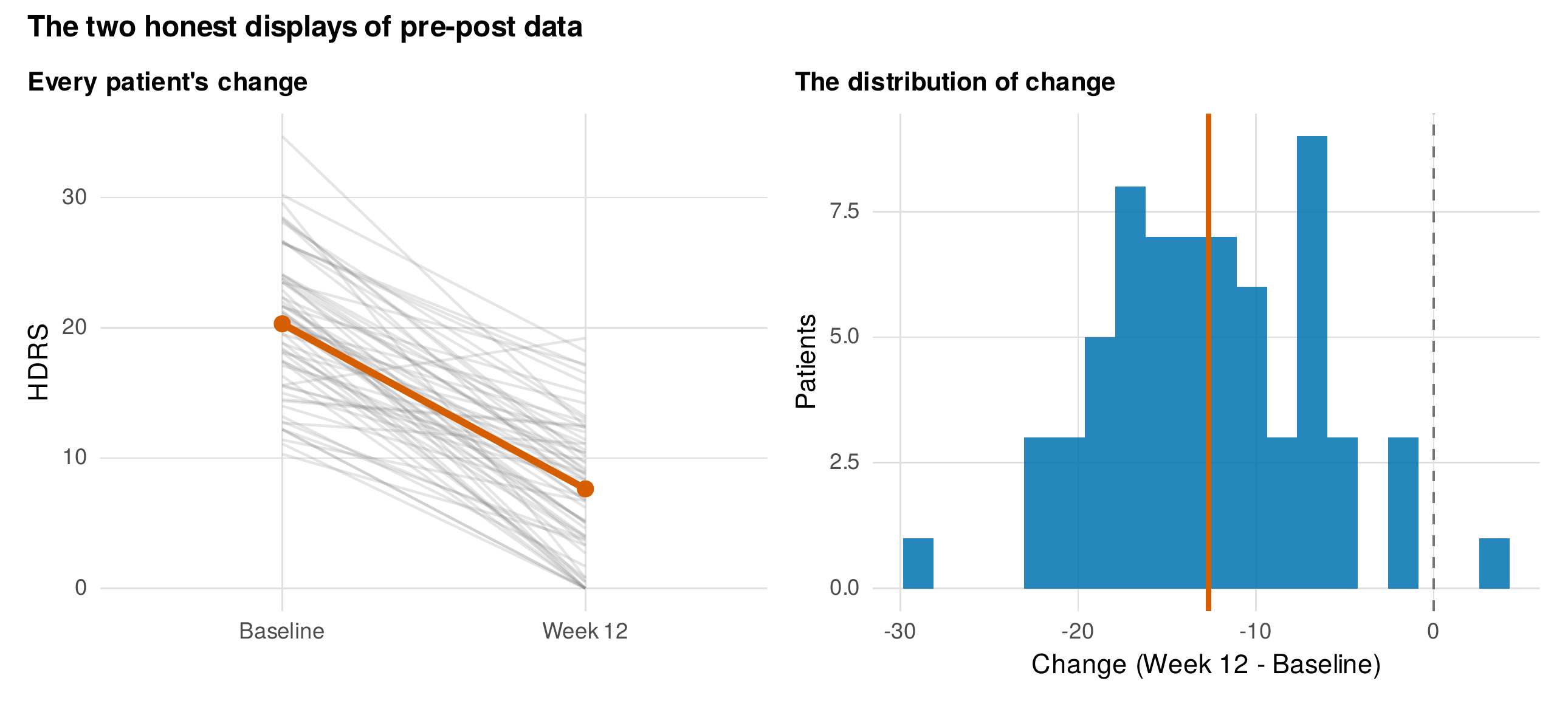
Note. Left: a slope chart connecting each treated patient’s baseline and week-12 HDRS, with the mean in bold; the spread of individual slopes is visible. Right: the distribution of change scores, whose mean (red line) is what the paired \(t\) test evaluates against zero (dashed line). The paired test is a one-sample test on these differences.
Foundations Box • Why pairing buys power: the variance of a difference
For paired measurements \((X_1, X_2)\) with variances \(\sigma_1^2, \sigma_2^2\) and correlation \(\rho\), the difference \(D = X_2 - X_1\) has variance \(\mathrm{Var}(D) = \sigma_1^2 + \sigma_2^2 - 2\rho\,\sigma_1\sigma_2\). When the two occasions are positively correlated, the subtracted term shrinks the variance of the difference, and for equal variances \(\sigma^2\) it becomes \(\mathrm{Var}(D) = 2\sigma^2(1 - \rho)\), which falls toward zero as \(\rho \to 1\). The paired \(t\) statistic is \(\bar{D}/(s_D/\sqrt{n})\), so a smaller \(\mathrm{Var}(D)\) yields a larger statistic and more power for the same mean change. This is the whole of the paired design’s advantage: by measuring the same people twice, it removes the stable between-person variance \(\sigma^2\) that an independent-groups comparison must carry as noise. An independent-groups test of the same change would face a difference variance of \(2\sigma^2\), the \(\rho = 0\) case.
The dependence of power on the pre-post correlation is not a technicality but the reason to prefer a within-person design, and Figure 10.2 makes it quantitative. For a fixed raw change and sample size, the paired design’s power rises steeply as the pre-post correlation grows, while an independent-groups analysis of the same data, unable to exploit the pairing, stays flat at the correlation-zero level. A study whose measurements correlate \(0.7\) across occasions can detect with a few dozen paired observations an effect that would require far more independent ones. When the outcome is ordinal or the differences are badly non-normal, the Wilcoxon signed-rank test is the common alternative, but it must be understood correctly: it is not simply a nonparametric \(t\) test but a test of whether the distribution of differences is symmetric about zero, and the cruder sign test asks only whether increases outnumber decreases. For paired binary outcomes, a change from one category to another, McNemar’s test evaluates whether the two kinds of discordant change are equally frequent, and it must not be confused with a measure of agreement such as kappa, because two occasions can agree strongly and still show systematic change. Table 10.1 maps outcome scale and question to the appropriate test.
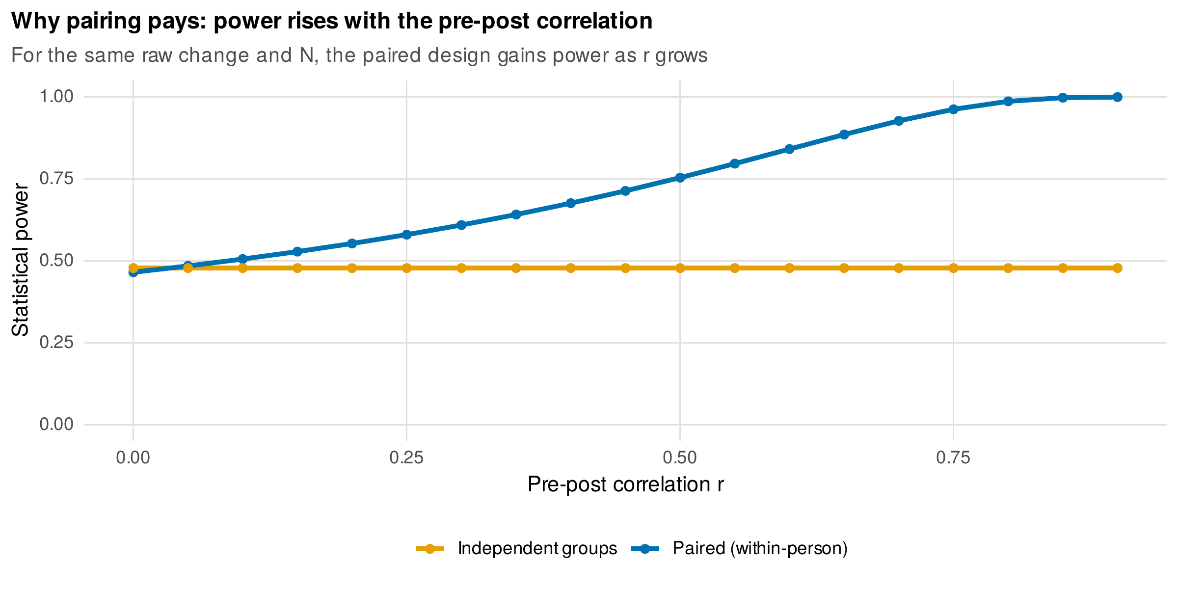
Note. Statistical power to detect a fixed raw change, for a paired (within-person) analysis and for an independent-groups analysis of the same data, as a function of the pre-post correlation. The paired design gains power as the correlation grows, because the correlated between-person variance is differenced away; the independent analysis cannot use the pairing and stays at the correlation-zero level.
Table 10.1. A two-occasion test selector.
| Outcome scale | Design and question | Test |
|---|---|---|
| Continuous | One group, mean change | Paired \(t\) (on differences) |
| Continuous, non-normal differences | One group, distributional shift | Wilcoxon signed-rank (symmetry) |
| Ordinal or direction only | One group, more up than down? | Sign test |
| Binary | One group, category switching | McNemar (exact or mid-\(p\)) |
| Continuous | Two groups, differential change | See Section 10.3 (change score vs. ANCOVA) |
Note. The paired \(t\) assumes approximate normality of the differences, not of the outcome. The signed-rank test evaluates symmetry of the differences, not equality of means, and the two can disagree when the difference distribution is skewed.
10.2 Effect Sizes for Paired Data
Reporting a paired analysis requires an effect size, and here a trap awaits that has corrupted meta-analyses. Two standardized effect sizes are in circulation for paired designs, and they answer different questions. The difference-metric standardized effect, \(d_z = \bar{D}/s_D\), divides the mean change by the standard deviation of the differences, and because that denominator is shrunk by the pre-post correlation (the Foundations box), \(d_z\) is large precisely when the correlation is high, so it is not comparable to a between-groups \(d\) and inflates when pooled with one. The raw-metric effect, \(d_{av} = \bar{D}/s_{av}\), divides instead by the average of the pretest and posttest standard deviations, and it is on the same scale as a between-groups effect and appropriate for meta-analysis (Dunlap et al., 1996; Morris & DeShon, 2002). The two can differ substantially: in the treatment arm of the trial, \(d_z = -2.12\) while \(d_{av} = -2.38\), and with a higher pre-post correlation the gap would widen. The rule is to report both, to state which is which, and never to enter a \(d_z\) into a meta-analysis of between-groups effects. Table 10.2 defines the paired effect sizes and their uses, and confidence intervals for any of them are obtained from the noncentral \(t\) distribution or by the bootstrap.
Table 10.2. Effect sizes for paired designs.
| Effect size | Denominator | When to report it |
|---|---|---|
| \(d_z\) | SD of the differences \(s_D\) | Within-study power and sample-size planning; not comparable to between-groups \(d\) |
| \(d_{av}\) | Average of pre and post SDs | The general-purpose paired effect; comparable across designs and safe for meta-analysis |
| \(d_{rm}\) | Corrected for the correlation | Meta-analytic pooling when the correlation is known (Morris & DeShon) |
| Rank-biserial | Rank-based | Companion to the Wilcoxon signed-rank test |
Note. The denominators differ, so the numbers differ; the choice is not cosmetic. Reporting \(d_z\) as if it were a between-groups \(d\) is a common and consequential error in meta-analysis.
10.3 Two Groups, Two Occasions: The Central Controversy
When two groups are each measured before and after, three analyses present themselves, and understanding why they can disagree is the intellectual core of the chapter. One may analyze the change scores, testing whether the groups differ in how much they changed; one may perform an analysis of covariance (ANCOVA), testing whether the groups differ at posttest after adjusting for the pretest; or one may compare posttest scores alone, ignoring the pretest. Under a randomized design with equal expected baselines the first two agree in expectation and ANCOVA is merely the more efficient, but when the groups are nonequivalent at baseline, the change-score and ANCOVA analyses estimate different quantities and can reach opposite conclusions. This is Lord’s paradox (Lord, 1967), and Figure 10.3 reproduces it numerically on constructed data. Two nonequivalent groups are each perfectly stable, their posttest means equal to their pretest means, so an analysis of change scores finds no group difference in change at all, an effect of \(0.5\) points that is not significant. Yet because the groups differ at baseline and the within-group regression of posttest on pretest has a slope below one, the ANCOVA finds a large and highly significant group difference of \(6.9\) points at posttest adjusting for the pretest. The data are identical; the verdicts are opposite.
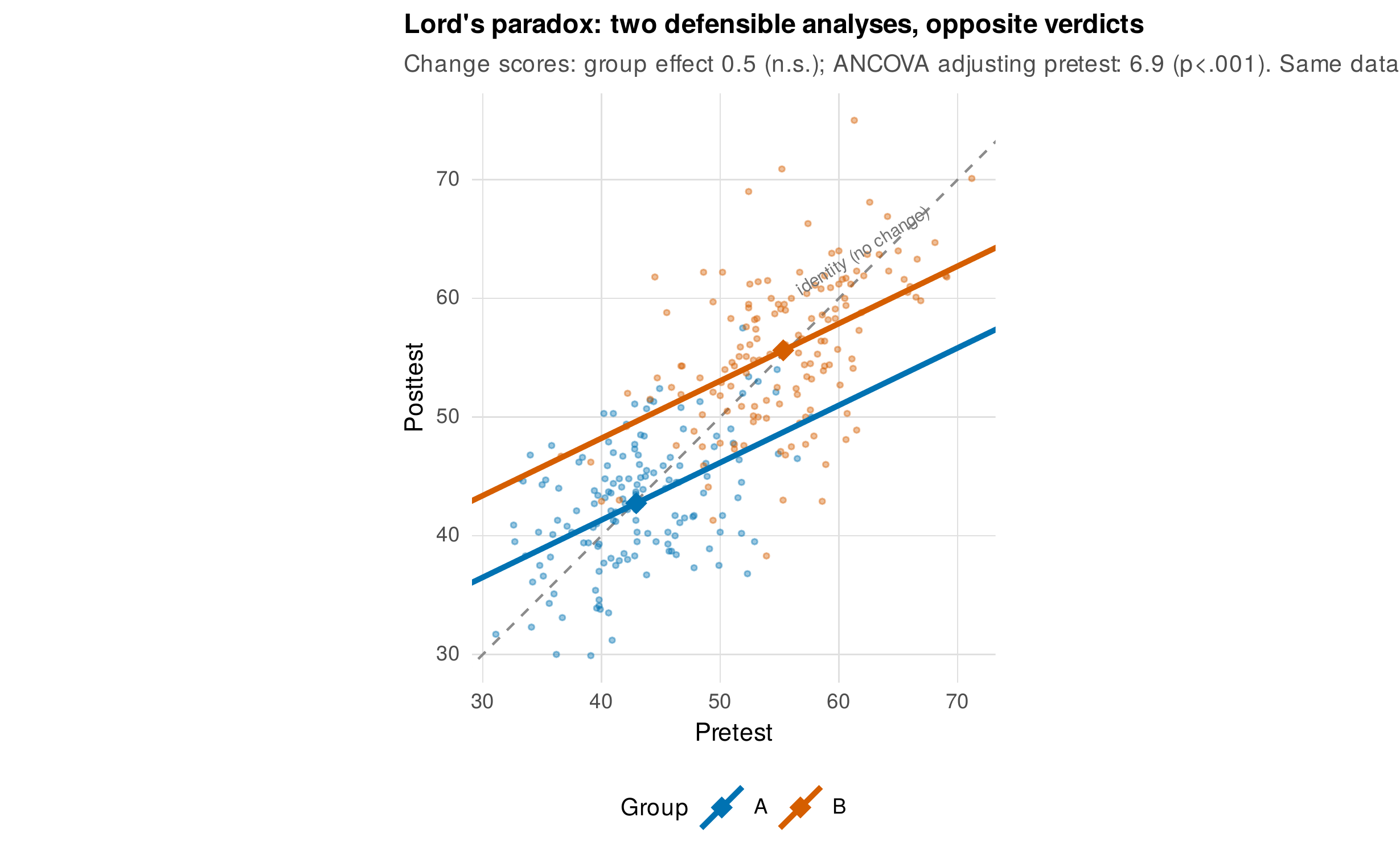
Note. Constructed data for two nonequivalent groups. Each group mean (diamond) lies on the identity line (dashed), so both groups are stable and a change-score analysis finds no group difference. The two analysis-of-covariance regression lines (solid, common slope) are vertically offset, so adjusting for the pretest yields a large group difference at posttest. The paradox is that both analyses are correct about different estimands.
The resolution is not to declare one analysis right but to see that each answers a different counterfactual question, and that the design determines which question is sensible. The change-score analysis assumes parallel trends, that absent any group effect the two groups would have changed by the same amount, which is the difference-in-differences logic of econometrics; it is defensible when the groups are on parallel trajectories that differ only in level. The ANCOVA assumes instead that, conditional on the pretest, group membership is unrelated to the posttest absent an effect, which is defensible when the pretest captures the relevant confounding. Under randomization both assumptions hold, the analyses agree, and ANCOVA is preferred for its greater power (van Breukelen, 2006; Senn, 2006). Under nonequivalent groups neither assumption is free, and the analyst must argue for one from substantive knowledge rather than let the software choose. Two further hazards deepen the difficulty. Regression to the mean, shown in Figure 10.4, is the tendency of extreme scorers to be less extreme on remeasurement purely because the two occasions are imperfectly correlated: with no intervention at all, the lowest tenth of pretest scorers rises toward the mean and the highest tenth falls toward it, so any analysis that conditions on baseline extremity risks mistaking this artifact for change. And when the pretest used as a covariate is itself measured with error, ANCOVA under-adjusts, because the attenuated regression coefficient cannot fully remove the baseline difference; Figure 10.5 shows that in nonequivalent groups this leaves a spurious group effect that grows as pretest reliability falls, from near zero at perfect reliability to nearly five points at a reliability of \(0.5\), when the true effect is zero. This attenuation is the case for adjusting on a latent pretest freed of measurement error, the structural-equation approach of Chapters 19 through 21. Table 10.3 is a decision framework.
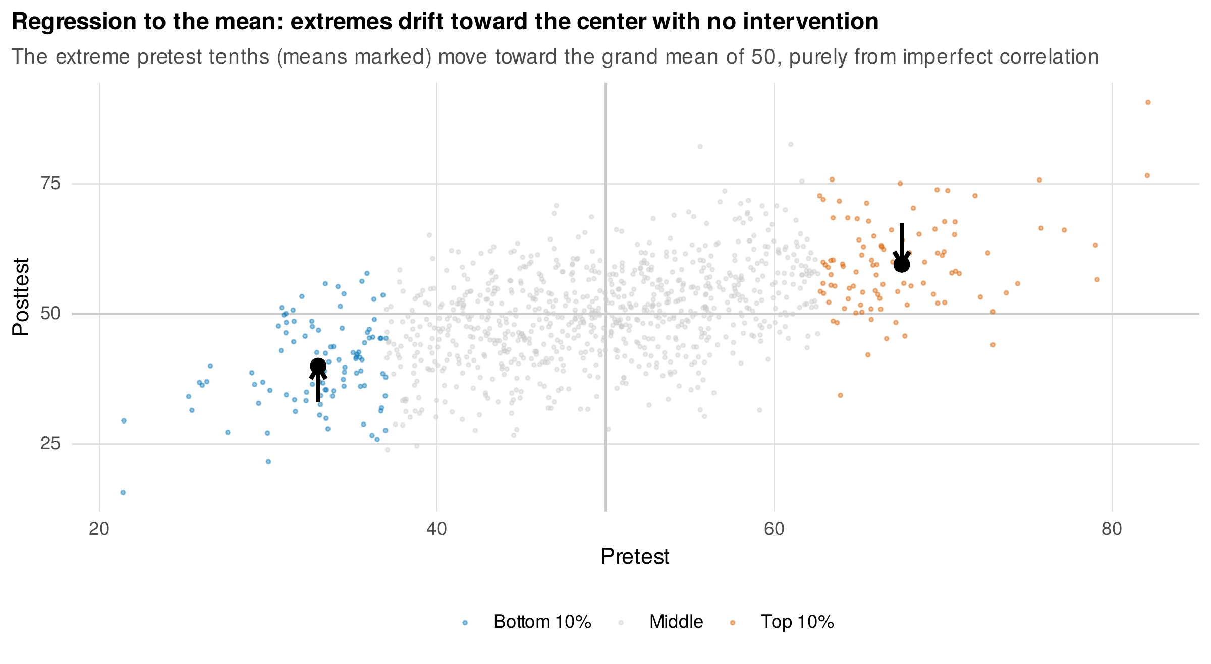
Note. Simulated data with no intervention, a grand mean of fifty, and an imperfect pre-post correlation. The lowest and highest tenths of pretest scorers (means marked with arrows) move toward the grand mean at posttest purely because the occasions are imperfectly correlated. Conditioning on baseline extremity can mistake this artifact for a real effect.
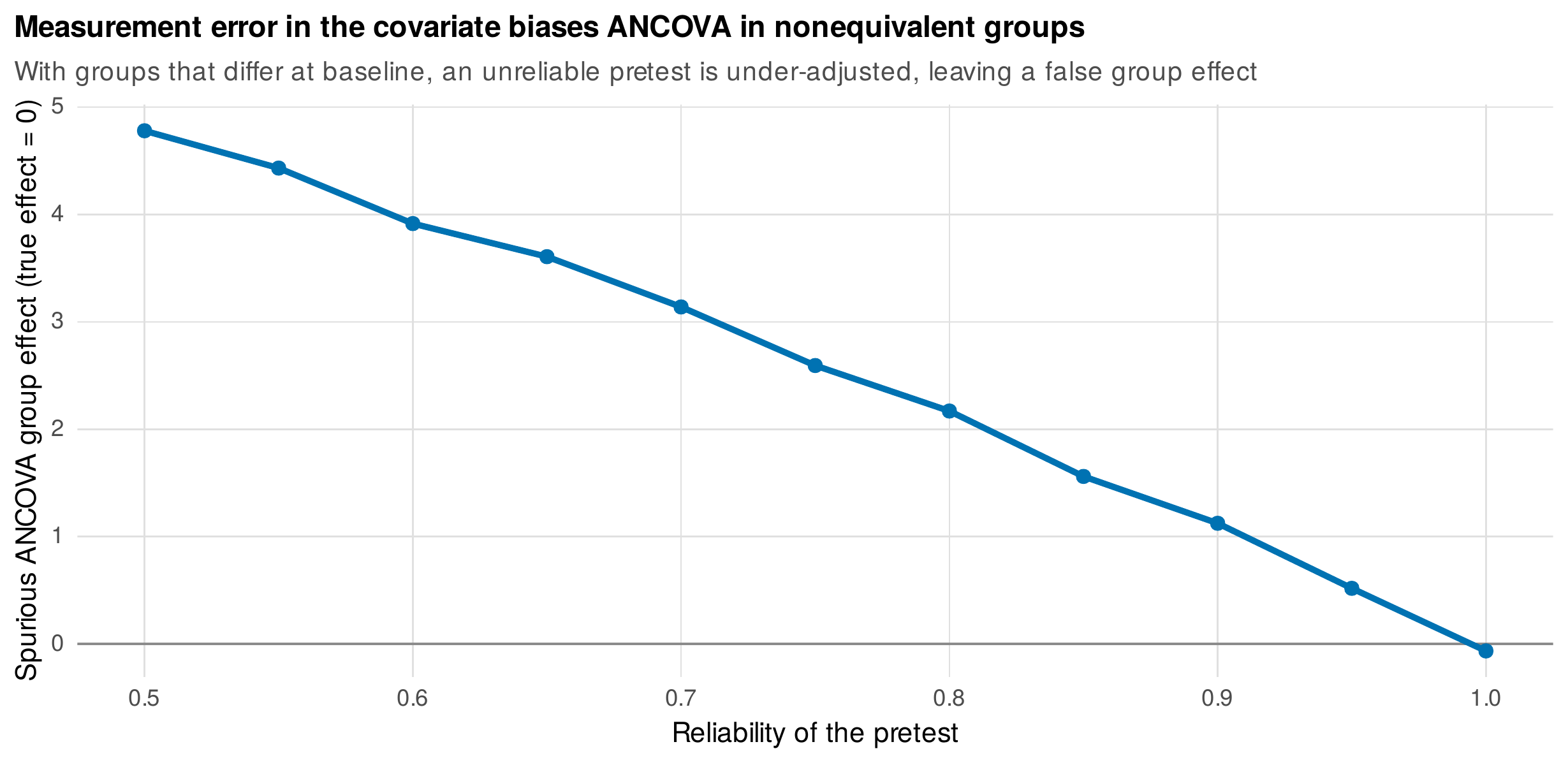
Note. Simulated nonequivalent groups with no true group effect on the posttest. As the reliability of the pretest covariate falls, the analysis of covariance under-adjusts for the baseline difference and reports a spurious group effect, reaching nearly five points at a reliability of one-half. The bias vanishes only when the pretest is perfectly reliable, motivating latent-variable adjustment.
Table 10.3. Change score versus ANCOVA: a decision framework.
| Situation | Preferred analysis | Reason |
|---|---|---|
| Randomized, equal baselines | ANCOVA | Both unbiased; ANCOVA more powerful |
| Nonequivalent groups, parallel trends plausible | Change score | Difference-in-differences estimand matches the design |
| Nonequivalent groups, pretest captures confounding | ANCOVA (latent if unreliable) | Conditional-exchangeability estimand; adjust for measurement error |
| Unreliable pretest | Latent-covariate adjustment | Observed ANCOVA under-adjusts (Figure 10.5) |
| Baseline selected on extremity | Neither uncritically | Regression to the mean contaminates both |
Note. The analyses estimate different quantities under different assumptions. The design, not a default, selects the estimand, and in nonequivalent groups the choice must be argued rather than automated.
10.4 Individual Change: The Reliable Change Index
Group-level tests answer whether the average person changed, but clinical and applied questions often concern whether this person changed, and by an amount beyond what measurement error alone would produce. The reliable change index (RCI) of Jacobson and Truax (1991) answers this by dividing a person’s observed change by the standard error of the difference, \(\mathrm{RCI} = (X_2 - X_1)/S_{\mathrm{diff}}\), where \(S_{\mathrm{diff}} = \sqrt{2}\,\mathrm{SE}_{\mathrm{meas}}\) and \(\mathrm{SE}_{\mathrm{meas}} = s_1\sqrt{1 - r_{xx}}\) depends on the scale’s reliability. A person whose reliable change index exceeds \(1.96\) in magnitude has changed by more than measurement error can readily explain. Combining this with a clinical cutoff that separates the functional from the dysfunctional range yields the Jacobson-Truax classification: a person is recovered if they changed reliably and crossed into the functional range, improved if they changed reliably but remain outside it, unchanged if their change is within measurement error, and deteriorated if they reliably worsened. Figure 10.6 plots every patient in the trial by baseline and endpoint, with the reliable-change bands and the remission cutoff drawn in, and it makes the classification visible: reliable change requires the point to fall beyond a band \(5.4\) HDRS points wide, and recovery requires it also to fall below the remission line. The two criteria are distinct, and Table 10.4 lays out the computation; the essential caution is that the reliability coefficient must match the scale and population, because an inappropriate reliability inflates or deflates every classification.
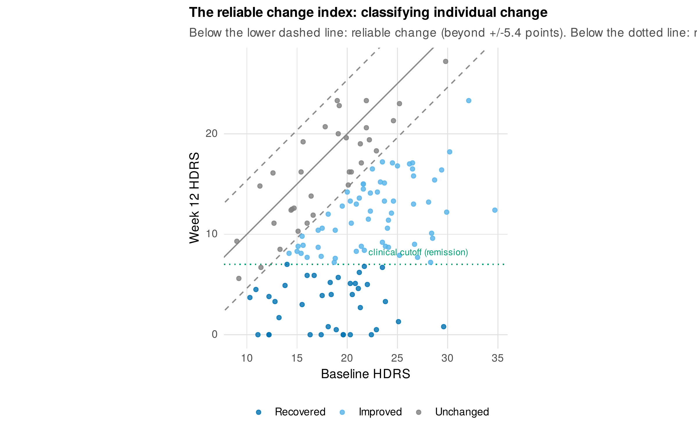
Note. Every patient by baseline and week-12 HDRS. The solid line is no change; points below the lower dashed line changed reliably (beyond a band of \(\pm5.4\) points set by the scale’s reliability); the dotted line is the remission cutoff. A patient below both lines is recovered; below the reliable-change band but above remission, improved. Reliable change and clinical significance are separate criteria.
Table 10.4. Components of the reliable change index.
| Quantity | Definition and role |
|---|---|
| \(\mathrm{SE}_{\mathrm{meas}} = s_1\sqrt{1 - r_{xx}}\) | Standard error of measurement; smaller when the scale is more reliable |
| \(S_{\mathrm{diff}} = \sqrt{2}\,\mathrm{SE}_{\mathrm{meas}}\) | Standard error of a difference of two measurements |
| \(\mathrm{RCI} = (X_2 - X_1)/S_{\mathrm{diff}}\) | Standardized change; \(|\mathrm{RCI}| > 1.96\) is reliable |
| Clinical cutoff | A criterion separating functional from dysfunctional scores |
| Classification | Recovered, improved, unchanged, or deteriorated, from RCI and cutoff jointly |
Note. Reliable change asks whether the change exceeds measurement error; clinical significance asks whether the person crossed a meaningful threshold. A person can meet either criterion without the other, so both are reported.
10.5 Establishing the Absence of Change
A nonsignificant paired test does not establish that nothing changed, because failing to reject the null is not evidence for it, and a study too small to detect a meaningful change will routinely return nonsignificance whatever the truth. To claim stability, one must test for it directly, and the tool is equivalence testing, specifically the two one-sided tests procedure (Lakens, 2017; Lakens et al., 2018). One first specifies an equivalence region, a range of change small enough to be considered trivial, chosen from the smallest effect size of interest as in Chapter 4, and then tests whether the observed change is significantly closer to zero than each bound. Figure 10.7 shows the logic applied to the control arm’s short-term stability: the ninety-percent confidence interval for the change lies entirely within a \(\pm2\)-point equivalence region, so the change is significantly smaller than the smallest effect of interest, and one may conclude equivalence rather than merely fail to find a difference. The equivalence bounds are the crux and must be justified substantively before the analysis, because a wide region makes equivalence easy to declare and a narrow one makes it nearly impossible; the bound encodes what counts as no meaningful change, and that is a scientific judgment, not a statistical one.
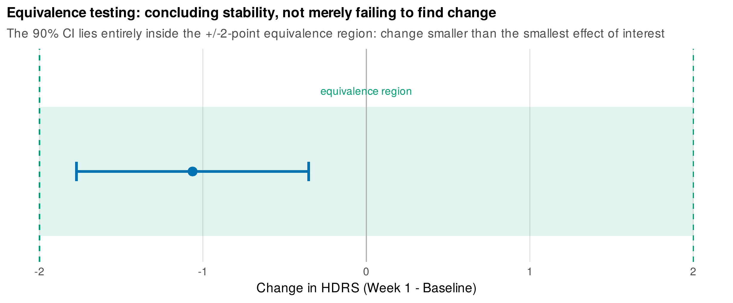
Note. The ninety-percent confidence interval for the control arm’s short-term change lies entirely within a \(\pm2\)-point equivalence region (shaded). Because the interval excludes both equivalence bounds, the change is significantly smaller than the smallest effect of interest, licensing a conclusion of equivalence. The bounds must be justified before the analysis.
10.6 Beyond Two Waves: What Cannot Be Learned
However carefully analyzed, two occasions carry a hard limit: they identify the amount of change but not its shape, and they cannot speak to the within-person dynamics that later chapters model. Figure 10.8 makes the limit concrete with three trajectories that share the same baseline and the same endpoint but differ entirely in between, one declining steadily, one dropping late, one dropping early and then leveling. A two-wave study measures only the endpoints and so cannot distinguish these processes, which are clinically and theoretically distinct: a steady responder, a late responder, and an early responder who plateaus tell different stories about mechanism and prognosis. This is not a failure of analysis but of design, and it is the reason the book moves beyond two waves. It also revives the difference-score reliability problem of Chapter 3, that a difference of two imperfectly reliable measurements can be less reliable than either, rehabilitated there and relevant here, and it sets up the analysis-of-variance methods of the next chapter and the growth models of Part IV, which require three or more occasions to identify a trajectory at all.
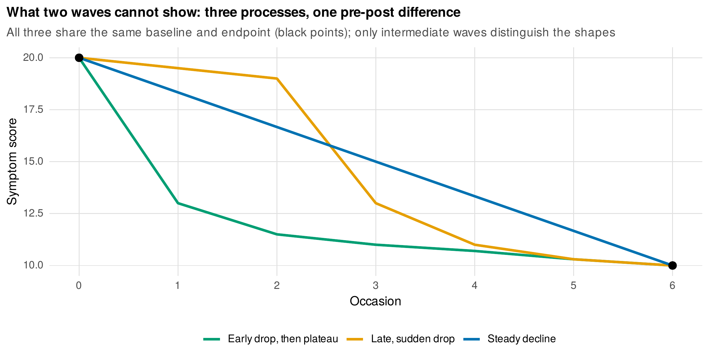
Note. Three trajectories with identical baseline and endpoint values (black points) but entirely different shapes: steady decline, a late sudden drop, and an early drop followed by a plateau. A two-occasion design observes only the endpoints and cannot distinguish these processes, which requires three or more waves.
10.7 Running the Analyses in R
The worked analyses use base R, whose t.test, wilcox.test, and mcnemar.test cover the paired tests, with effect sizes computed directly. The paired test is a one-sample test on the differences, and reporting both effect sizes is a two-line calculation.
library(dplyr); library(tidyr)
rct <- readRDS("Examples/data/therapy_rct.rds")
pp <- rct |> filter(week %in% c(0, 11)) |>
  pivot_wider(names_from = week, values_from = hdrs, names_prefix = "w",
              id_cols = c(patient_id, arm)) |>
  filter(!is.na(w0), !is.na(w11)) |> mutate(change = w11 - w0)

trt <- filter(pp, arm == "Treatment")
t.test(trt$w11, trt$w0, paired = TRUE)              # paired t on the differences
dz  <- mean(trt$change) / sd(trt$change)            # difference-metric d
dav <- mean(trt$change) / mean(c(sd(trt$w0), sd(trt$w11)))   # raw-metric d
The three two-group analyses are three linear models, and Lord’s paradox is reproduced by fitting all three to the nonequivalent-groups data and comparing the group coefficient.
ld <- readRDS("Examples/data/lord_demo.rds")
lm(change ~ group, data = ld)                       # change-score analysis
lm(post ~ pre + group, data = ld)                   # ANCOVA (adjust pretest)
lm(post ~ group, data = ld)                         # posttest only
The reliable change index is a direct calculation from the scale’s reliability, and the classification follows from the index and a clinical cutoff. The equivalence test is the two one-sided tests procedure, comparing a ninety-percent confidence interval to the equivalence bounds.
rel <- 0.86                                         # published scale reliability
se_meas <- sd(pp$w0) * sqrt(1 - rel); s_diff <- sqrt(2) * se_meas
pp <- pp |> mutate(RCI = change / s_diff,
  class = case_when(RCI <= -1.96 & w11 <= 7 ~ "Recovered",
                    RCI <= -1.96            ~ "Improved",
                    RCI >=  1.96            ~ "Deteriorated",
                    TRUE                    ~ "Unchanged"))

# --- Equivalence (TOST): is the change within a +/- 2-point region? ---
d <- na.omit(with(filter(rct, arm == "Control", week %in% c(0,1)),
                  tapply(hdrs, week, mean)))        # illustrative; see script
The complete analysis, including the power-versus-correlation curve, the regression-to-the-mean and measurement-error simulations, and the full reliable-change classification, is the shipped script ch10_analysis_V01.R; the figures are drawn by ch10_figures_V01.R, and the paradox data are archived as lord_demo. For readers using a graphical package, the effectsize and TOSTER packages compute the paired effect sizes and the equivalence test respectively, and reproduce the values shown here.
Software Note • effect-size and equivalence tooling
Base R covers every test in this chapter, but two packages streamline the reporting. The effectsize package computes \(d_z\), \(d_{av}\), and their confidence intervals from a fitted paired test, removing the chance of pairing the wrong denominator with the wrong label, and it reports rank-based effect sizes for the nonparametric tests. The TOSTER package implements the two one-sided tests procedure and its power analysis, taking the equivalence bounds in raw or standardized units. Readers migrating from point-and-click software will find the paired \(t\) under a “paired-samples” menu and ANCOVA under a general-linear-model or regression menu; the mapping is exact, but the responsibility to choose change score or ANCOVA by design, not by default, remains with the analyst.
10.8 Reporting a Two-Occasion Analysis
A two-occasion result is reported with the test, the mean change and its interval, an effect size correctly labeled, and, for a trial, the CONSORT participant flow. A model paragraph for the trial reads: “Among the \(66\) treated patients with complete pre-post data, HDRS scores declined from baseline to week 12 by a mean of \(12.67\) points, \(t(65) = 17.1\), \(p < .001\), a large effect (\(d_{av} = 2.38\); \(d_z = 2.12\)), with the difference-metric and raw-metric standardized effects reported separately. The control arm declined by \(6.80\) points (95% CI \([5.40, 8.20]\)). Because the trial was randomized, the between-arm comparison used analysis of covariance adjusting for baseline, the more powerful of the two unbiased analyses. Individual change was classified by the reliable change index using a published reliability of \(.86\) (\(S_{\mathrm{diff}} = 2.74\)); \(30\) of \(66\) treated patients recovered and a further \(31\) improved reliably, against \(8\) and \(32\) in the control arm.” Every element is present, the effect sizes are disambiguated, and the choice of ANCOVA is justified by the design rather than asserted. The pitfalls box below collects the errors this reporting avoids.
Common Pitfall • three errors in two-occasion analysis
First, meta-analyzing \(d_z\): because \(d_z\) is inflated by the pre-post correlation, entering it into a meta-analysis of between-groups effects overstates the effect, sometimes grossly; report and pool \(d_{av}\) or a correlation-corrected effect. Second, treating “controlling for baseline” as automatically virtuous: in a nonequivalent-groups design, adjusting for a baseline that differs between groups estimates a counterfactual that may not exist, and with an unreliable pretest it under-adjusts (Figure 10.5); the adjustment must be argued from the design, and when a reviewer demands it reflexively, the defensible response cites Lord’s paradox and the estimand at issue. Third, a reliable change index with the wrong reliability: using a reliability from a different scale, sample, or interval miscalibrates every classification, so the coefficient must match the instrument and population in hand.
10.9 Common Misconceptions
Several beliefs about two-occasion analysis mislead. The first is that the paired \(t\) test requires a normally distributed outcome; it requires only approximate normality of the difference scores, and is robust to mild departures at moderate sample sizes. The second is that ANCOVA is always superior to the change score; the two estimate different quantities, and under nonequivalent groups the superiority claim is empty because there is no assumption-free answer, as Lord’s paradox shows. The third is that a nonsignificant pre-post test means no change occurred; absence of evidence is not evidence of absence, and a claim of stability requires an equivalence test with justified bounds. The fourth is that a significant reliable change index means clinically meaningful recovery; reliable change and clinical significance are separate criteria, and a person can change reliably without crossing any meaningful threshold. A recurring practical question, how to answer a reviewer who demands baseline adjustment in an observational pre-post design, is met not by refusal but by naming the estimand: state which counterfactual the adjustment assumes, show whether the design supports it, and offer the change-score analysis as the complementary estimand under parallel trends.
Chapter Summary
Two-occasion designs are ubiquitous and instructive, and their central lesson is that the analysis encodes the question. The paired \(t\) test is a one-sample test on difference scores whose power advantage comes from differencing away between-person variance, and that advantage grows with the pre-post correlation (Figures 10.1, 10.2); the Wilcoxon and McNemar tests handle non-normal and binary outcomes with hypotheses of their own. Paired effect sizes come in a difference metric (\(d_z\)) and a raw metric (\(d_{av}\)) that must not be confused, because \(d_z\) inflates with the correlation and corrupts meta-analyses. The controversy of change score versus analysis of covariance is dramatized by Lord’s paradox, in which the same nonequivalent-groups data yield no group difference in change but a large difference by ANCOVA (Figure 10.3), because the two analyses assume different counterfactuals; regression to the mean and pretest measurement error further complicate the adjustment (Figures 10.4, 10.5), and the design must select the estimand. Individual change is classified by the reliable change index against measurement error and a clinical cutoff (Figure 10.6), stability is established by equivalence testing rather than by a nonsignificant result (Figure 10.7), and two waves, however analyzed, identify the amount of change but never its shape (Figure 10.8).
Where to Go Next
The two-occasion case is the seed of everything that follows. The paired \(t\) test is the simplest within-person model, an intercept-only model on difference scores, and the next chapter generalizes it to three or more occasions through repeated-measures analysis of variance, while Part IV reframes both as special cases of the mixed model, where the change score and the covariate adjustment reappear as modeling choices rather than separate procedures. The difference-in-differences logic of the change-score analysis returns in the cross-lagged panel debates of Chapters 20 and 21, where the same estimand controversy is fought at the latent level, and the case for adjusting on an error-free latent pretest is taken up by the structural-equation methods of Chapters 19 through 21. The reliable-change and clinical-significance ideas reappear in the clinical applications of Chapter 33. The single lesson carried forward is that two defensible analyses can answer different questions, and that the analyst’s first duty is to name the question before choosing the model.
Exercises
- 10.1 When they coincide. Show algebraically that the change-score and analysis-of-covariance estimators of a group difference are equal when the groups have equal baseline means and the within-group pre-post regression slope is one, and identify which assumption randomization secures.
- 10.2 Reproduce the paradox. On the provided
lord_demodata, run all three two-group analyses, state the claim each party would make, and adjudicate between them by making the counterfactual assumptions explicit. - 10.3 A full paired analysis. For one arm of
therapy_rct, conduct the paired test, report both standardized effect sizes with intervals, and produce the slope chart and difference distribution. - 10.4 Reliable change. Classify all patients by the reliable change index under two different reliability coefficients, and report how many classifications change and in which direction.
- 10.5 Design an equivalence test. For a claim of “no deterioration” after treatment discontinuation, justify equivalence bounds from a smallest effect of interest, and state what sample size the two one-sided tests procedure would require to detect equivalence with adequate power.
References
Allison, P. D. (1990). Change scores as dependent variables in regression analysis. Sociological Methodology, 20, 93–114. https://doi.org/10.2307/271083
Barnett, A. G., van der Pols, J. C., & Dobson, A. J. (2005). Regression to the mean: What it is and how to deal with it. International Journal of Epidemiology, 34(1), 215–220. https://doi.org/10.1093/ije/dyh299
Cronbach, L. J., & Furby, L. (1970). How we should measure “change”: Or should we? Psychological Bulletin, 74(1), 68–80. https://doi.org/10.1037/h0029382
Dunlap, W. P., Cortina, J. M., Vaslow, J. B., & Burke, M. J. (1996). Meta-analysis of experiments with matched groups or repeated measures designs. Psychological Methods, 1(2), 170–177. https://doi.org/10.1037/1082-989X.1.2.170
Holland, P. W., & Rubin, D. B. (1983). On Lord’s paradox. In H. Wainer & S. Messick (Eds.), Principals of modern psychological measurement: A festschrift for Frederic M. Lord (pp. 3–25). Lawrence Erlbaum Associates.
Jacobson, N. S., & Truax, P. (1991). Clinical significance: A statistical approach to defining meaningful change in psychotherapy research. Journal of Consulting and Clinical Psychology, 59(1), 12–19. https://doi.org/10.1037/0022-006X.59.1.12
Lakens, D. (2017). Equivalence tests: A practical primer for t tests, correlations, and meta-analyses. Social Psychological and Personality Science, 8(4), 355–362. https://doi.org/10.1177/1948550617697177
Lakens, D., Scheel, A. M., & Isager, P. M. (2018). Equivalence testing for psychological research: A tutorial. Advances in Methods and Practices in Psychological Science, 1(2), 259–269. https://doi.org/10.1177/2515245918770963
Lord, F. M. (1967). A paradox in the interpretation of group comparisons. Psychological Bulletin, 68(5), 304–305. https://doi.org/10.1037/h0025105
Morris, S. B., & DeShon, R. P. (2002). Combining effect size estimates in meta-analysis with repeated measures and independent-groups designs. Psychological Methods, 7(1), 105–125. https://doi.org/10.1037/1082-989X.7.1.105
Rogosa, D. R. (1988). Myths about longitudinal research. In K. W. Schaie, R. T. Campbell, W. Meredith, & S. C. Rawlings (Eds.), Methodological issues in aging research (pp. 171–209). Springer.
Senn, S. (2006). Change from baseline and analysis of covariance revisited. Statistics in Medicine, 25(24), 4334–4344. https://doi.org/10.1002/sim.2682
van Breukelen, G. J. P. (2006). ANCOVA versus change from baseline had more power in randomized studies and more bias in nonrandomized studies. Journal of Clinical Epidemiology, 59(9), 920–925. https://doi.org/10.1016/j.jclinepi.2006.02.007