Chapter 11
Repeated Measures ANOVA and MANOVA
The analysis of variance for repeated measures is the ANOVA tradition’s answer to change, and it remains the default in experimental psychology and the language most reviewers expect. This chapter treats it with the respect a still-useful tool deserves and the precision its assumptions demand. The aim is twofold: to teach the method properly, its decomposition of variance, its load-bearing sphericity assumption and the corrections that rescue it, its contrasts and mixed designs and its multivariate alternative; and to delimit it exactly, so that the move to mixed models in Part IV is motivated by understanding rather than fashion. The repeated-measures analysis of variance is not an obsolete rival of the mixed model but a constrained special case of it, powerful within a narrow domain of balanced, complete, categorically-timed data, and the chapter closes by demonstrating, not merely asserting, the five limitations that make the general model necessary.
Learning Objectives
After working through this chapter, you should be able to: (1) decompose the repeated-measures sums of squares and explain how a within-subject design removes individual differences from the error term; (2) state the sphericity assumption exactly, test it, and apply the Greenhouse-Geisser and Huynh-Feldt corrections by default; (3) analyze mixed between-within factorial designs and interpret their interaction through contrasts and simple effects with the correct error terms; (4) conduct trend analysis with orthogonal polynomial contrasts and connect it to growth curves; (5) choose between the corrected univariate and the multivariate approaches and defend the choice; (6) compute and interpret partial and generalized eta-squared; and (7) enumerate and demonstrate the five structural limitations that motivate the mixed model.
11.1 The Within-Subject Advantage, Formalized
The power of a repeated-measures design comes from a partition of variance that a between-subjects design cannot perform. When every person is measured on every occasion, the total variation can be split first into a between-persons part, reflecting stable individual differences in overall level, and a within-persons part, and the between-persons variation, which in a between-subjects design would inflate the error term, is instead removed from it. Figure 11.1 shows this partition for the treatment arm of the therapy trial: the total sum of squares divides into a large between-persons component that is set aside, and a within-persons component that divides again into the occasion effect, the signal, and a residual within-persons error against which that signal is tested. Because the error term no longer carries the between-person variance, the test of the occasion effect is far more sensitive than an equivalent between-subjects comparison would be. This is the same advantage the paired \(t\) test enjoyed in Chapter 10, now generalized from two occasions to \(k\). Table 11.1 states the expected mean squares that justify the \(F\) ratio, and the crucial line is the last: the occasion effect is tested against the within-persons residual, whose expected mean square under the null equals the error variance alone.
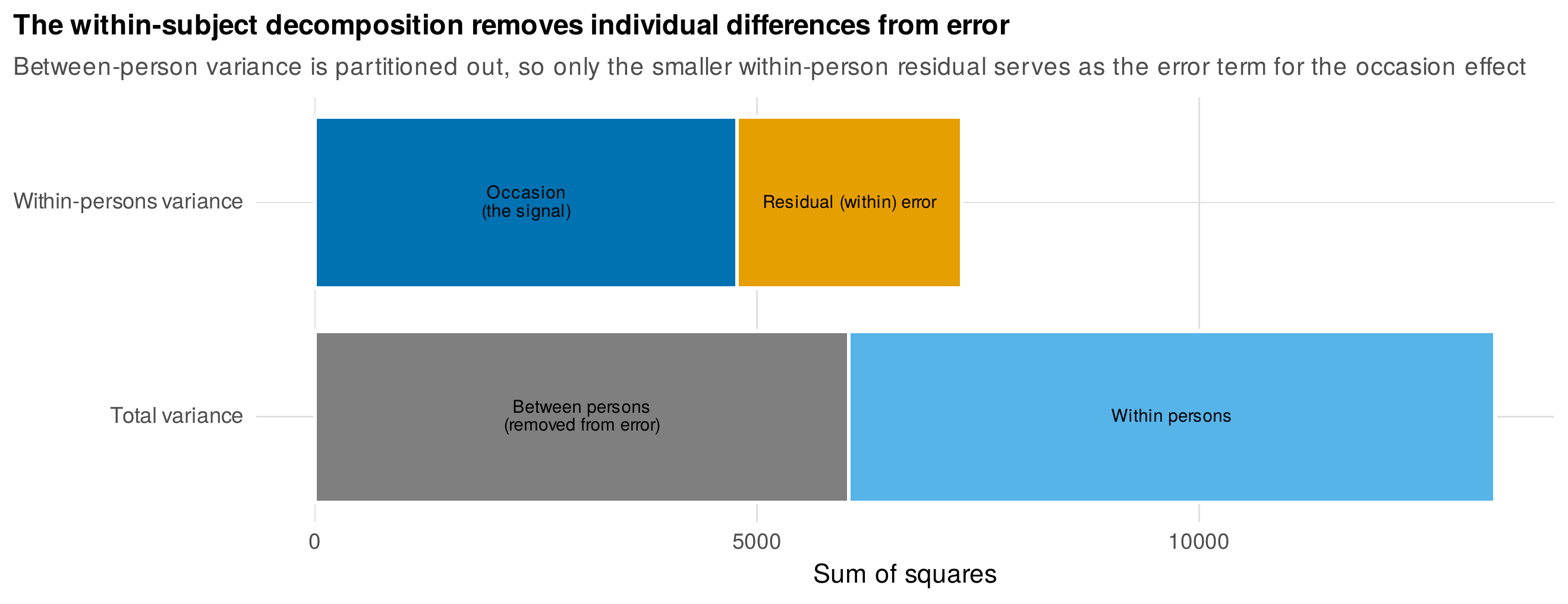
Note. The total sum of squares for the treatment arm partitions into a between-persons part (set aside) and a within-persons part, and the within-persons part divides into the occasion effect and the residual error. Because the between-person variance is removed, the occasion effect is tested against a small within-person error, which is the source of the repeated-measures design’s power.
Table 11.1. Expected mean squares for the one-way repeated-measures design.
| Source | \(df\) | Expected mean square | \(F\) |
|---|---|---|---|
| Between persons (\(S\)) | \(n-1\) | \(\sigma^2_e + k\,\sigma^2_S\) | |
| Occasion (\(A\)) | \(k-1\) | \(\sigma^2_e + n\,\theta^2_A\) | \(\mathrm{MS}_A/\mathrm{MS}_{SA}\) |
| Error (\(S \times A\)) | \((n-1)(k-1)\) | \(\sigma^2_e\) |
Note. \(\sigma^2_S\) is the between-persons variance, \(\theta^2_A\) the occasion effect, and \(\sigma^2_e\) the residual. The occasion effect is tested against the person-by-occasion interaction, whose expected mean square is the error variance alone. Writing the design this way, a random person effect plus a fixed occasion effect, already expresses it as a constrained mixed model, the point Part IV generalizes.
The expected-mean-square structure of Table 11.1 is worth reading twice, because it reveals that the repeated-measures analysis of variance is a mixed model in disguise. A random person effect, contributing the between-persons variance \(\sigma^2_S\), plus a fixed occasion effect, is exactly the random-intercept model of Chapter 13, and the \(F\) test the design performs is the test that model would perform under one specific covariance assumption. Recognizing this now removes any sense that Part IV replaces the present chapter; it generalizes it, relaxing the one assumption examined next.
11.2 Sphericity: The Load-Bearing Assumption
The validity of the repeated-measures \(F\) test rests not on the familiar homogeneity of variance but on the stronger and more fragile assumption of sphericity: that the variances of all pairwise differences between occasions are equal. Equivalently, after removing occasion and person means, the covariance among occasions has the compound symmetry form, equal variances and equal covariances. Longitudinal data almost never satisfy this, because occasions closer in time are more strongly correlated than occasions far apart, an autoregressive structure under which differences between distant occasions are more variable than differences between adjacent ones. Figure 11.2 shows the violation directly in the treatment data: the variance of the paired difference grows steadily with the separation between the two occasions, whereas sphericity would require every point to lie on the dashed line. The departure from sphericity is quantified by epsilon (\(\varepsilon\)), which equals one under perfect sphericity and falls toward \(1/(k-1)\) as the violation worsens (Box, 1954); for these data the Greenhouse-Geisser estimate is \(\varepsilon = 0.87\), and Mauchly’s test of sphericity is significant (\(W = 0.79\), \(p = .004\)).
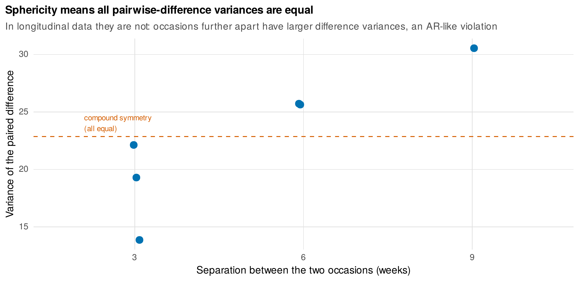
Note. The variance of the difference between two occasions, plotted against how far apart they are, for the treatment arm. Sphericity requires these to be equal (dashed line), but they grow with separation, the autoregressive violation typical of longitudinal data. The departure is summarized by \(\varepsilon < 1\).
The consequence of ignoring a sphericity violation is a badly inflated Type I error rate, because the uncorrected \(F\) uses degrees of freedom that are too large when the differences are correlated. Figure 11.3 demonstrates this with a simulation under a true null: as the autoregressive correlation among occasions rises and \(\varepsilon\) falls, the uncorrected test rejects a true null far more than five percent of the time, reaching seven percent at strong correlation, while the two standard corrections restore control by shrinking the degrees of freedom by the factor \(\varepsilon\). The Greenhouse-Geisser correction (Greenhouse & Geisser, 1959) multiplies both degrees of freedom by the estimated \(\varepsilon\) and is slightly conservative; the Huynh-Feldt correction (Huynh & Feldt, 1976) uses a less biased estimate that tracks the nominal rate more closely. The temptation is to test sphericity with Mauchly’s procedure and correct only when it is significant, but this two-stage strategy is itself a source of inflation, because Mauchly’s test has low power and frequently fails to detect real violations, licensing an uncorrected test that then over-rejects. The defensible policy is therefore to correct by default, applying Greenhouse-Geisser or Huynh-Feldt to every within-subject \(F\) regardless of Mauchly’s verdict, since when sphericity does hold, \(\varepsilon\) is near one and the correction costs almost nothing.
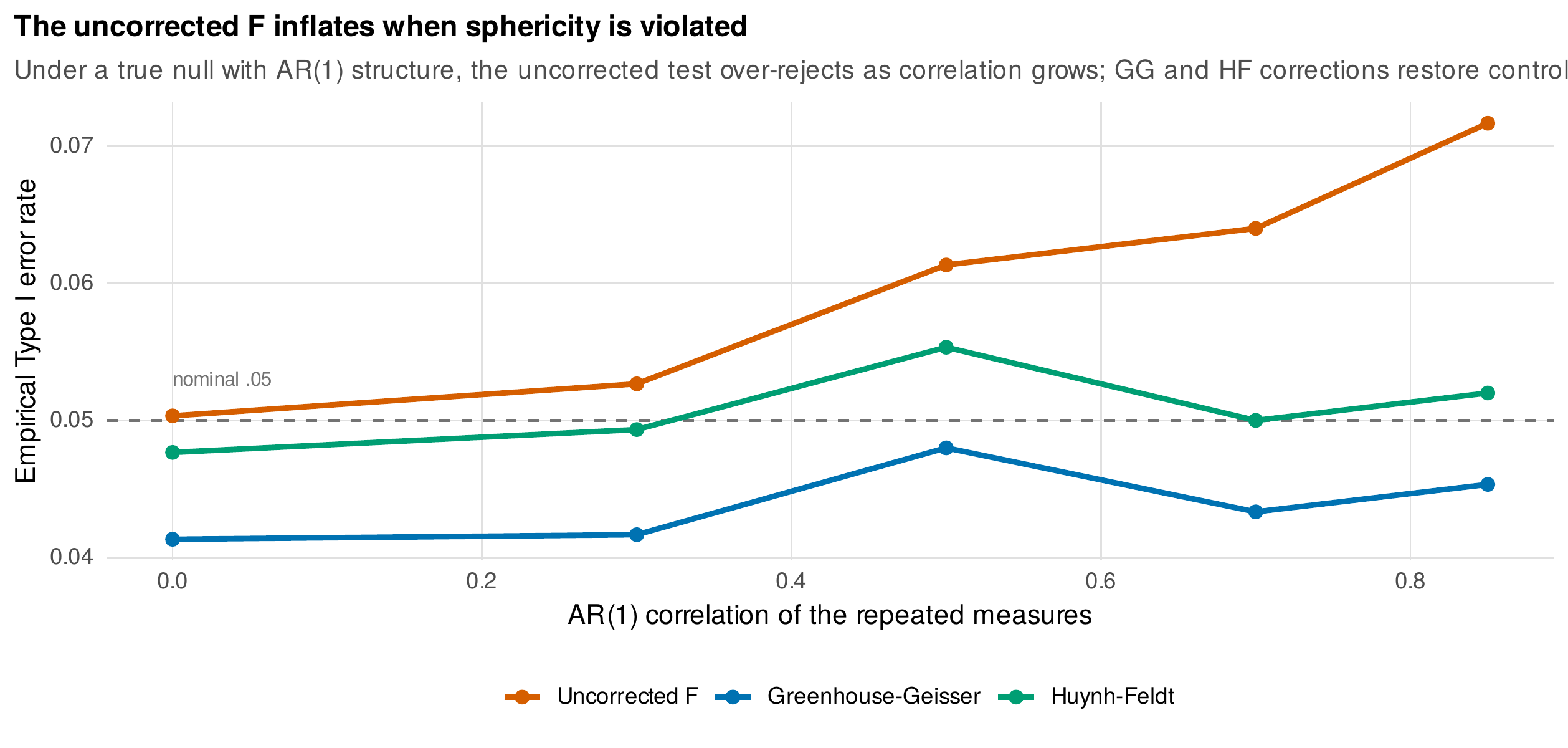
Note. Empirical Type I error rate under a true null with autoregressive covariance among four occasions, as a function of the correlation, from a simulation. The uncorrected \(F\) over-rejects as correlation grows and sphericity worsens; the Greenhouse-Geisser (slightly conservative) and Huynh-Feldt corrections hold the rate near the nominal five percent. This is the case for correcting by default.
11.3 Contrasts, Trends, and Planned Comparisons
An omnibus occasion effect answers only that the means differ somewhere, and the interpretable questions are usually about the shape of change, which orthogonal polynomial contrasts address by partitioning the occasion effect into a linear trend, a quadratic trend, and higher components. Figure 11.4 shows the contrast weights: the linear contrast tests a steady increase or decrease, the quadratic a single bend, and each is a single-degree-of-freedom comparison. These contrasts have a decisive practical virtue: because each is a single derived score per person, tested as a one-sample comparison, each carries its own error term and is therefore free of the sphericity assumption that troubles the omnibus test. Applied to the treatment arm, the trend analysis is unambiguous: the linear contrast is large and highly significant (\(t = -16.7\), \(p < .001\)), while the quadratic adds little (\(t = -1.59\), \(p = .12\)) and the cubic nothing, so the decline in symptoms is essentially a straight line. Figure 11.5 overlays the linear and the linear-plus-quadratic fits on the observed means and confirms that the straight line captures the occasion effect. The bridge to Part IV is explicit here: a set of polynomial trend contrasts is a fixed-effects growth curve without random slopes, the description of an average trajectory that the latent growth models of Chapter 19 will endow with individual variation.
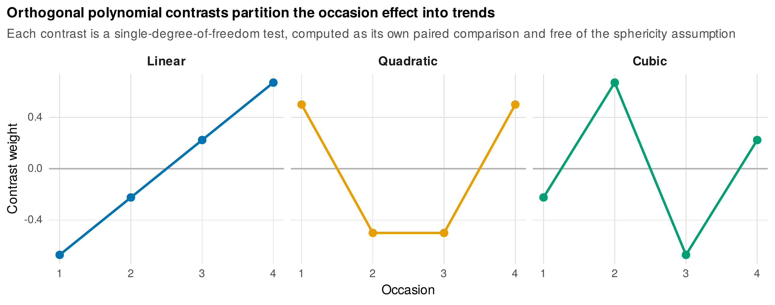
Note. The weights of the linear, quadratic, and cubic contrasts across four occasions. Each contrast is a single-degree-of-freedom test computed as its own paired comparison, and so is free of the sphericity assumption. The linear contrast tests a steady trend, the quadratic a single bend.
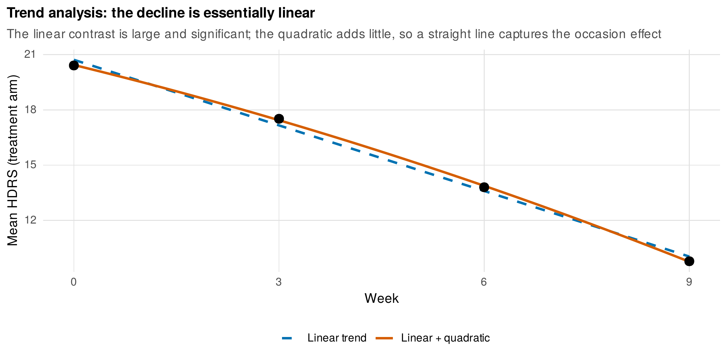
Note. Observed mean HDRS at four weeks for the treatment arm (points), with the fitted linear trend (dashed) and the linear-plus-quadratic fit (solid). The linear contrast is significant and the quadratic is not, so a straight line captures the average trajectory. Polynomial trend contrasts are fixed-effects growth curves without random slopes.
11.4 Mixed Factorial Designs
The canonical evaluation design crosses a between-subjects factor with the within-subjects occasion factor, and its signature test is the interaction. Figure 11.6 shows the two arms of the therapy trial across four waves, both as overlaid profiles and as the difference trajectory that is the trial’s actual estimand. The group-by-time interaction tests whether the arms change differently over time, and it is the formal treatment-effect test: here it is large and highly significant, \(F(3, 444) = 17.7\), \(p < .001\), with the corresponding multivariate parallelism test agreeing (Wilks \(\Lambda = 0.79\), \(p < .001\)). A significant interaction does not, however, mean the treatment worked at every wave, and the honest follow-up decomposes it into simple effects, the arm difference tested within each occasion. Figure 11.7 shows that the arms are equivalent at baseline, as randomization ensures, and diverge progressively thereafter, so the interaction reflects a treatment benefit that emerges over time rather than a baseline imbalance. The error terms for such follow-ups must be chosen with care, because a between-groups simple effect at one occasion uses a different error stratum than a within-group trend, and using the pooled omnibus error for every comparison is a common mistake. The mixed factorial design also imports a distinction from experimental psychology that longitudinal researchers must keep clear: in a true repeated-measures experiment, occasion is a manipulated condition and order effects must be controlled by counterbalancing, whereas in longitudinal observation occasion is time itself and cannot be counterbalanced, so carryover is a substantive feature rather than a nuisance to be designed away.
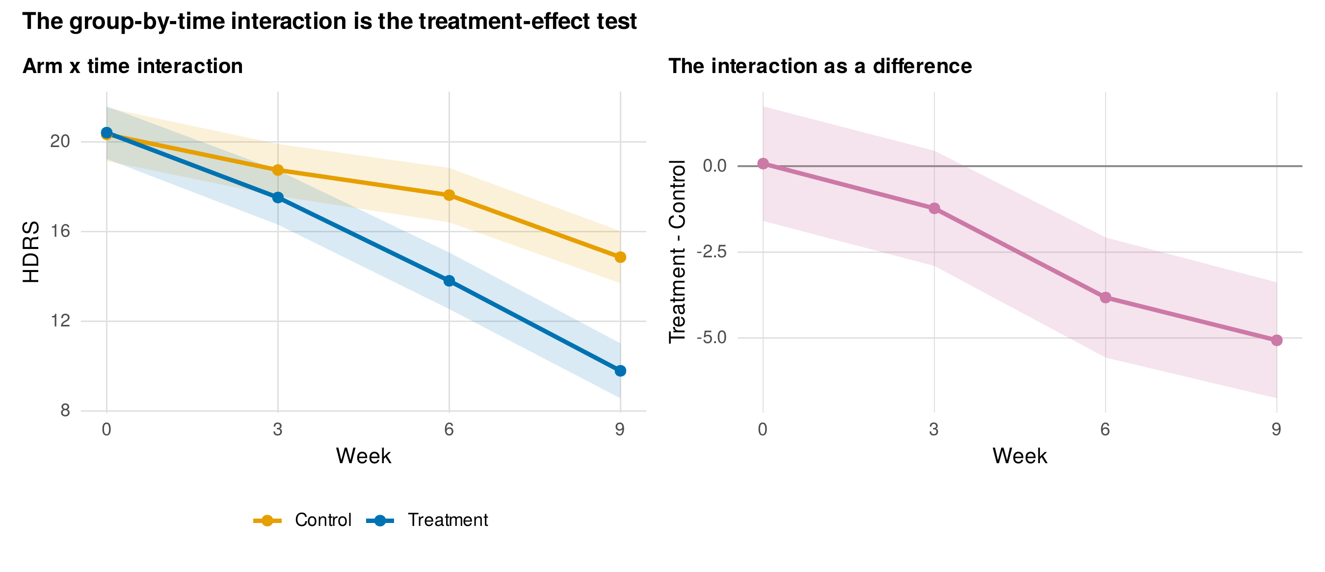
Note. Left: mean HDRS for the two arms across four waves, with confidence ribbons. Right: the treatment-minus-control difference trajectory. The interaction, which tests whether the arms change differently, is the formal treatment-effect test and is displayed most directly as the difference trajectory (as in Chapter 8).
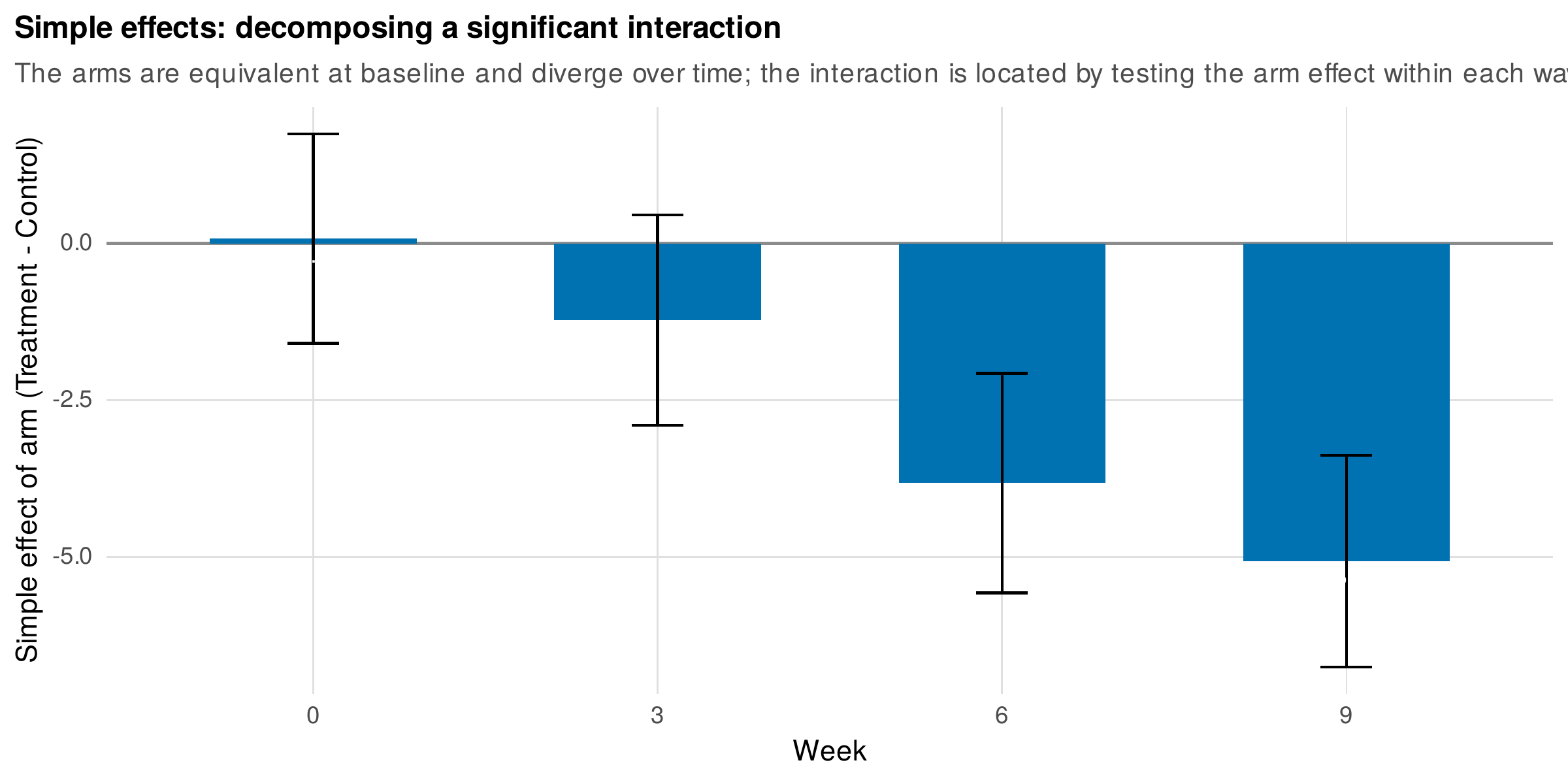
Note. The arm difference (treatment minus control) tested within each wave, with confidence intervals. The arms are equivalent at baseline and diverge over time, so the interaction reflects an emerging treatment benefit rather than a baseline imbalance. Simple effects locate an interaction; each uses its appropriate error term.
11.5 The Multivariate Approach
An alternative to correcting the univariate \(F\) is to abandon the sphericity assumption altogether by treating the \(k\) occasions as a \(k\)-dimensional multivariate outcome, the multivariate analysis of variance (MANOVA) approach (O’Brien & Kaiser, 1985). Its within-subject tests, reported as Wilks’s lambda, Pillai’s trace, or related statistics, make no assumption about the covariance structure among occasions, requiring instead multivariate normality and, crucially, complete data. This freedom is not without cost: when the sample is small relative to the number of occasions the multivariate test can be less powerful than the corrected univariate one, so the classic guidance favors the corrected univariate approach at small samples and the multivariate approach when the sample is ample and sphericity is badly violated (Davidson, 1972; Algina & Keselman, 1997). The multivariate framing has an especially interpretable form in profile analysis, which poses three questions of the group profiles, illustrated in Figure 11.8: parallelism, whether the groups have the same shape of change, which is the interaction; levels, whether they differ in average height, which is the between-groups main effect; and flatness, whether they change at all, which is the within-subjects main effect. For the therapy data all three are answered decisively, the profiles are non-parallel, differ in level, and are not flat, which together say that the arms started similarly, both improved, and the treatment arm improved more. Table 11.2 guides the choice between the two approaches.
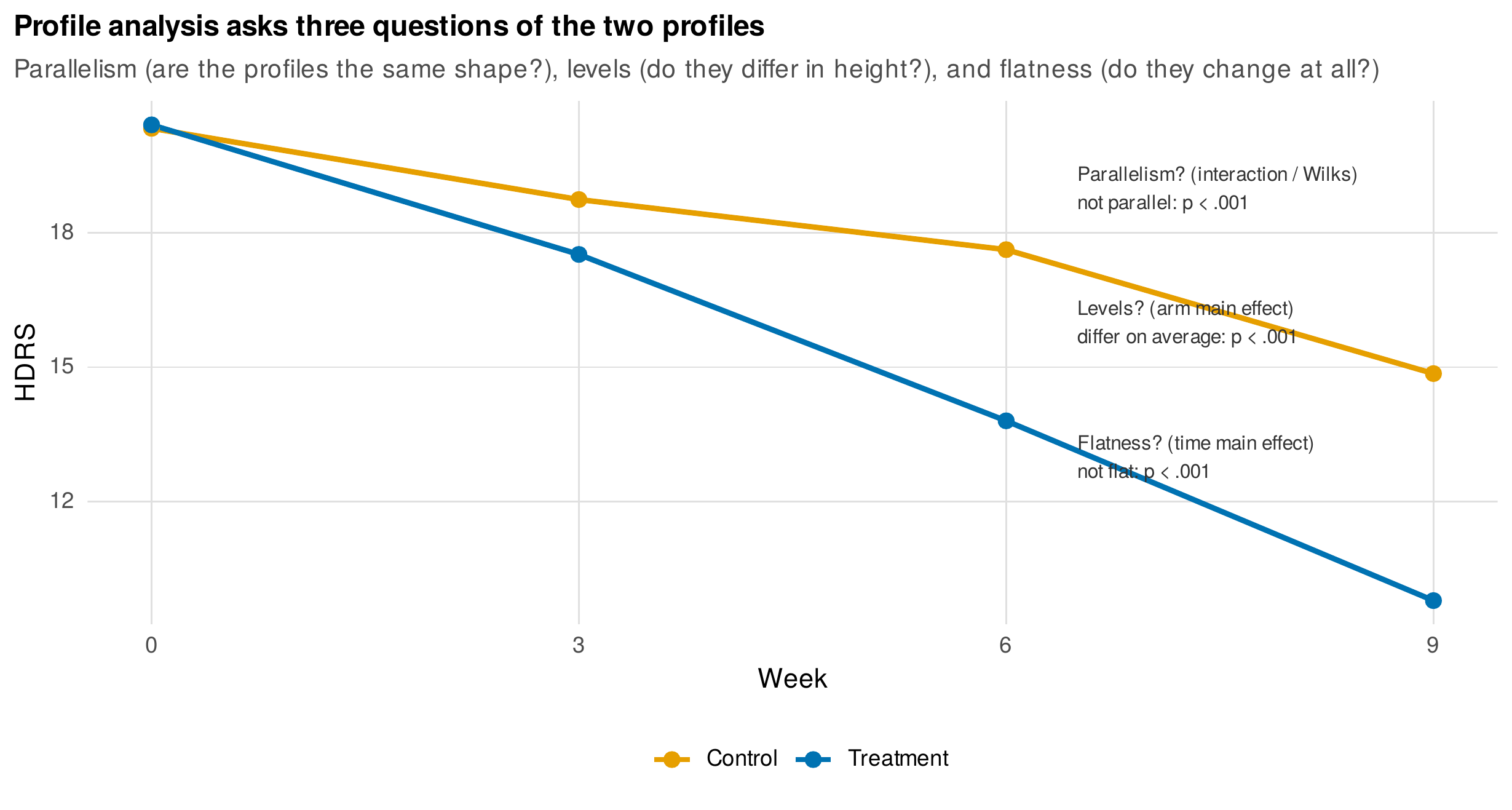
Note. The two arm profiles across weeks, annotated with the three profile-analysis questions: parallelism (the interaction, are the profiles the same shape), levels (the between-groups main effect, do they differ in height), and flatness (the within-subjects main effect, do they change). Profile analysis is the interpretable face of the multivariate approach.
Table 11.2. Corrected univariate versus multivariate: a selection guide.
| Situation | Preferred approach |
|---|---|
| Small \(n\) relative to occasions | Corrected univariate (Greenhouse-Geisser / Huynh-Feldt) |
| Ample \(n\), severe sphericity violation | Multivariate (Wilks, Pillai) |
| Interest in trend shape | Polynomial contrasts (sphericity-free either way) |
| Missing occasions | Neither; use the mixed model (Part IV) |
| Interpretable group-profile questions | Profile analysis (parallelism, levels, flatness) |
Note. Both approaches assume complete, balanced data. When occasions are missing, individually timed, or continuous, neither applies and the mixed model is required. Pillai’s trace is the most robust multivariate statistic under assumption violations.
11.6 Effect Sizes and Reporting
A repeated-measures result is reported with an effect size, and the choice between the two common ones matters for cumulative science. Partial eta-squared expresses an effect relative to itself plus its own error, and because that denominator excludes variance from other factors and from between-person differences, partial eta-squared is inflated in within-subject designs and, worse, is not comparable across designs with different factor structures. Generalized eta-squared (Olejnik & Algina, 2003; Bakeman, 2005) uses a denominator that includes the between-person and error variance that would be present in any design, and so is comparable across between-subjects, within-subjects, and mixed designs, which is why it is the recommended default for repeated measures. The two can differ greatly: for the treatment-by-time interaction the partial eta-squared is \(.11\) while the generalized eta-squared is \(.04\), and reporting the partial value as if it were comparable to a between-subjects effect would overstate the interaction. Effect sizes for the specific contrasts, a standardized linear-trend effect for instance, are often more informative than the omnibus value. Table 11.3 defines the options, and Table 11.4 is the reporting checklist, whose non-negotiable elements are the corrected degrees of freedom, the value of \(\varepsilon\), and a generalized effect size.
Table 11.3. Effect sizes for repeated-measures designs.
| Effect size | Denominator | Use |
|---|---|---|
| Partial \(\eta^2\) | Effect \(+\) its own error | Within-study; not comparable across designs |
| Generalized \(\eta^2\) | Effect \(+\) between-person and error variance | Recommended; comparable across designs |
| \(\omega^2\) (generalized) | Less biased version | When bias correction matters |
| Contrast \(d\) | SD of the contrast | Trend-specific, often the most informative |
Note. Generalized eta-squared is the book’s recommendation because its denominator restores the variance components that partial eta-squared removes, making effects comparable across the between-subjects, within-subjects, and mixed designs a literature contains.
Table 11.4. Reporting checklist for repeated-measures designs.
| Element | What to report |
|---|---|
| Corrected test | \(F\) with Greenhouse-Geisser or Huynh-Feldt degrees of freedom, and the value of \(\varepsilon\) |
| Effect size | Generalized eta-squared for each effect |
| Sphericity | That correction was applied by default (not conditional on Mauchly) |
| Interaction follow-up | Simple effects or contrasts with appropriate error terms and multiplicity control |
| Trend | Polynomial contrasts where shape is of interest |
| Missing data | How incomplete cases were handled, and the resulting \(n\) |
Note. Reporting the uncorrected degrees of freedom, omitting \(\varepsilon\), or giving only partial eta-squared are the common omissions. The checklist aligns with APA expectations for repeated-measures designs.
11.7 What Repeated-Measures ANOVA Cannot Do
The chapter’s respect for the method makes its limits the more instructive, and five of them, demonstrated in the gallery of Figure 11.9, together make the mixed model of Part IV necessary rather than merely fashionable. First, the design requires complete, balanced data, so a single missing occasion removes a person entirely by listwise deletion, and in the therapy data requiring all twelve weeks retains only \(134\) of the enrolled patients, discarding both cases and statistical power for a reason Chapter 6 showed to be avoidable. Second, occasion must be categorical, so a design in which people are measured at individually varying times, common in observational and intensive studies, cannot be expressed at all. Third, the model admits no individual differences in change: it estimates a single average trajectory, and the variance in slopes across people, often the substantive quantity of interest, is invisible to the omnibus \(F\). Fourth, its covariance assumptions are a rigid menu, compound symmetry or the multivariate unstructured extreme, with none of the intermediate autoregressive and heterogeneous structures a mixed model can fit and compare. Fifth, it cannot accommodate a time-varying covariate, a predictor that itself changes across occasions, because its design matrix has no place for one. Table 11.5 is the reader’s Rosetta stone, translating each repeated-measures concept into its mixed-model equivalent, and it is the bridge that the next chapters cross; the same table reappears in Chapter 13.
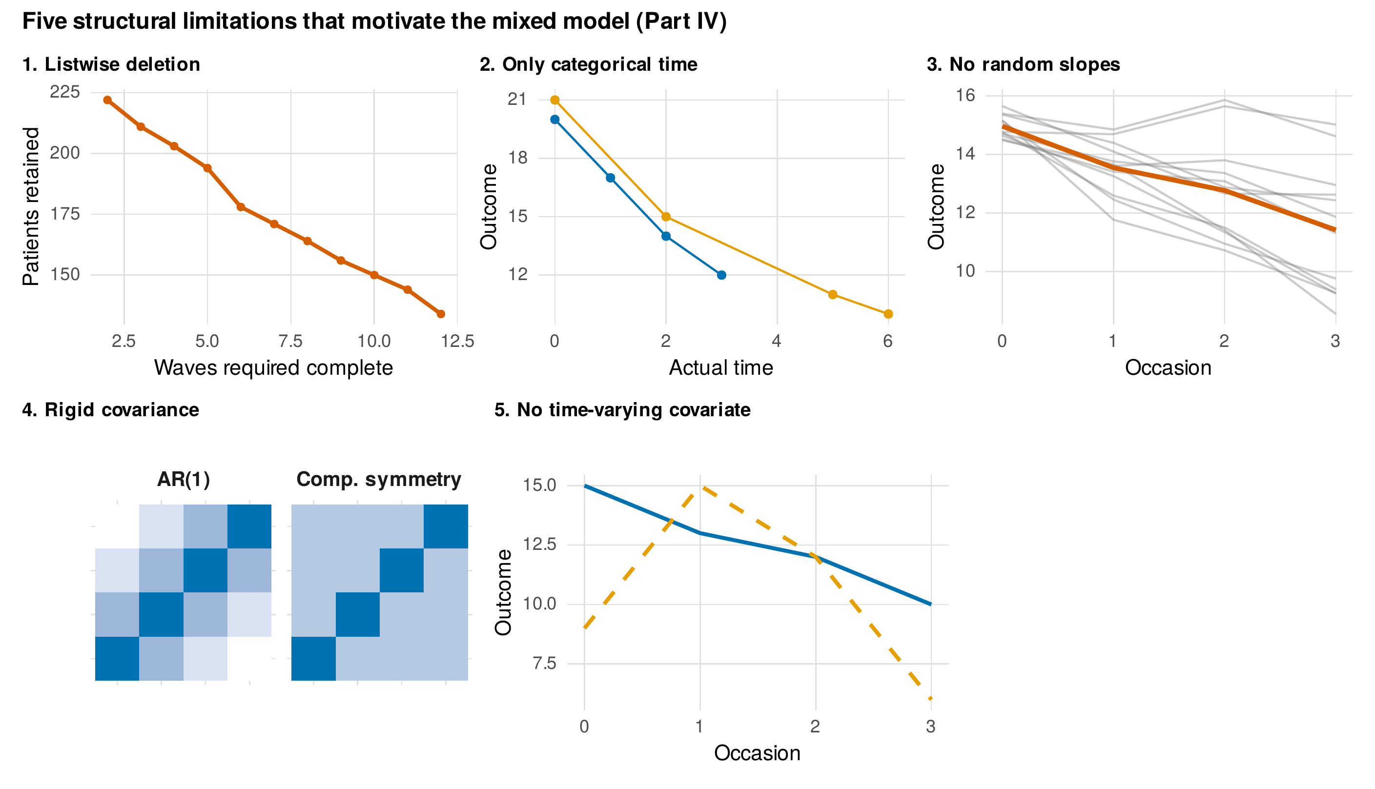
Note. (1) Listwise deletion discards a patient for any missing occasion, so requiring more complete waves sheds cases. (2) Only categorical, equally-spaced time can be expressed, not individually-varying measurement times. (3) A single average trajectory is estimated; individual differences in slope are invisible. (4) The covariance menu is rigid. (5) A time-varying covariate cannot be included. Each is removed by the mixed model of Part IV.
Table 11.5. Translating repeated-measures ANOVA into the mixed model.
| Repeated-measures ANOVA | Mixed-model equivalent |
|---|---|
| Between-persons sum of squares | Random intercept, (1 | person) |
| Compound symmetry assumption | Random-intercept-only covariance |
| Sphericity correction (\(\varepsilon\)) | A fitted covariance structure (AR, unstructured) |
| Occasion as a factor | Fixed effect of time |
| Polynomial trend contrast | Fixed polynomial time (no random slope) |
| Group-by-time interaction | Fixed group-by-time interaction |
| (Not available) individual slope variance | Random slope, (time | person) |
| Listwise deletion of incomplete cases | Direct likelihood over observed data (FIML) |
| Categorical, balanced time only | Continuous, individually-varying time |
| (Not available) time-varying covariate | A level-1 time-varying predictor |
Note. Each row on the left is a special case or limitation of the general model on the right. The repeated-measures analysis of variance is the mixed model constrained to a random intercept, categorical balanced time, and complete data.
11.8 Running the Analysis in R
Base R performs the repeated-measures analysis of variance through aov with an Error stratum that separates the between-person and within-person error terms, and the sphericity machinery is a short calculation on the covariance matrix of the repeated measures.
library(dplyr); library(tidyr)
rct <- readRDS("Examples/data/therapy_rct.rds")
w <- rct |> filter(week %in% c(0, 3, 6, 9)) |>
  pivot_wider(names_from = week, values_from = hdrs, names_prefix = "w",
              id_cols = c(patient_id, arm)) |> filter(complete.cases(across(everything())))
long <- w |> pivot_longer(starts_with("w"), names_to = "occ", values_to = "y") |>
  mutate(occ = factor(occ), pid = factor(patient_id), arm = factor(arm))

# --- Mixed factorial: between (arm) x within (occ), correct error strata ---
fit <- aov(y ~ arm * occ + Error(pid / occ), data = long)
summary(fit)                                        # arm in pid stratum; occ, arm:occ within
The Greenhouse-Geisser epsilon is computed from the covariance of orthonormal within-subject contrasts, and Mauchly’s test is available for a multivariate linear model; the polynomial trends and the multivariate profile tests follow the same contrast logic.
Y <- as.matrix(dplyr::filter(w, arm == "Treatment")[, c("w0","w3","w6","w9")])
k <- ncol(Y); n <- nrow(Y); C <- t(contr.poly(k))   # (k-1) x k orthonormal contrasts
lam <- eigen(C %*% cov(Y) %*% t(C))$values           # eigenvalues of the contrast covariance
eps_gg <- sum(lam)^2 / ((k - 1) * sum(lam^2))        # Greenhouse-Geisser epsilon
mauchly.test(lm(Y ~ 1), X = ~1)                      # sphericity test

# --- Polynomial trend contrasts: each is its own single-df, sphericity-free test ---
apply(contr.poly(k), 2, function(w) t.test(Y %*% w)$p.value)   # linear, quadratic, cubic

# --- Multivariate / profile analysis (parallelism = arm x time interaction) ---
D <- Y <- as.matrix(w[, c("w0","w3","w6","w9")]) %*% contr.poly(4)
summary(manova(D ~ w$arm), test = "Wilks")           # no sphericity assumption
The complete analysis, including the hand-computed decomposition of a small dataset, the Type I error simulation, and the generalized eta-squared calculations, is the shipped script ch11_analysis_V01.R, with figures drawn by ch11_figures_V01.R. Readers using the afex package obtain the same corrected tests and effect sizes with a single call, and emmeans handles the contrasts and simple effects with multiplicity control; the base-R route is shown here so the mechanism is visible.
Software Note • the error-stratum trap, and the afex convenience
The single most common base-R error in repeated-measures analysis is omitting or misspecifying the Error term, which causes aov to pool the within-person and between-person variation into one wrong error stratum and to report a badly anticonservative \(F\). The correct specification, Error(pid / occ), tells R that occasions are nested within persons, so that the between-subjects factor is tested against the person stratum and the within-subjects factor against the person-by-occasion stratum. The afex package removes this hazard by taking a single formula with explicit within and between factors, applying Greenhouse-Geisser by default, and returning generalized eta-squared, and it enforces Type III sums of squares for consistency with the multi-way designs. Readers migrating from menu-driven software will find its output maps directly onto the general-linear-model repeated-measures tables they know, including the sphericity and correction rows.
11.9 Interpreting and Reporting the Results
A repeated-measures result is reported with corrected degrees of freedom, a generalized effect size, and the follow-up that locates any interaction. A model paragraph for the trial reads: “A \(2 \times 4\) mixed analysis of variance with arm as a between-subjects factor and week as a within-subjects factor was conducted on \(150\) patients with complete data at weeks 0, 3, 6, and 9. Greenhouse-Geisser corrections were applied to all within-subjects tests (\(\varepsilon = .87\)). The main effect of week was significant, \(F(2.6, 385) = 152.0\), \(p < .001\), generalized \(\eta^2 = .24\), as was the arm-by-week interaction, \(F(2.6, 385) = 17.7\), \(p < .001\), generalized \(\eta^2 = .04\). Trend analysis showed the within-arm change to be predominantly linear. Simple-effects tests indicated that the arms did not differ at baseline but diverged progressively thereafter, with the treatment arm improving more.” The corrected degrees of freedom, the reported \(\varepsilon\), the generalized effect size, and the interaction decomposition are all present, and the pitfalls box collects the errors this reporting avoids.
Common Pitfall • four errors in repeated-measures analysis
First, test-then-correct: running Mauchly’s test and correcting only when it is significant inflates Type I error, because the test is underpowered; correct by default. Second, partial eta-squared across designs: comparing a within-subjects partial eta-squared to a between-subjects one is invalid, because their denominators differ; report generalized eta-squared for comparability. Third, main effects under a crossover interaction: when profiles cross, a main effect averages over opposite simple effects and can be meaningless or misleading; interpret the interaction first. Fourth, ignoring counterbalancing: in an experimental repeated-measures design, treating order as irrelevant confounds carryover with the occasion effect; counterbalance and, ideally, test for order.
11.10 Common Misconceptions
Several beliefs about the repeated-measures analysis of variance mislead. The first is that the Greenhouse-Geisser correction is conservative, so it can be skipped when Mauchly’s test is nonsignificant; the correction is nearly costless when sphericity holds and essential when it does not, and skipping it on the strength of an underpowered test is exactly the inflation to avoid. The second is that MANOVA is the modern replacement for the univariate approach; the two are alternatives with complementary strengths, and at the small samples common in psychology the corrected univariate test is often the more powerful. The third is that a significant group-by-time interaction means the treatment worked at every wave; the interaction says only that the groups changed differently, and simple effects are required to locate where. The fourth is that repeated-measures ANOVA and the mixed model are rival philosophies; the former is a constrained special case of the latter, and the choice between them is practical, not ideological. A recurring question, whether unequal group sizes are a problem, is answered reassuringly for the between-subjects factor, which tolerates imbalance, and pointedly for the within-subjects factor, where the real difficulty is not unequal groups but missing occasions, which the design cannot accommodate at all.
Chapter Summary
The repeated-measures analysis of variance partitions variance so that stable individual differences are removed from the error term (Figure 11.1), which is the source of its power and, as its expected mean squares reveal, marks it as a constrained mixed model. Its validity rests on sphericity, the equality of all pairwise-difference variances, which longitudinal data violate through their autoregressive structure (Figure 11.2); ignoring the violation inflates Type I error (Figure 11.3), so the Greenhouse-Geisser or Huynh-Feldt correction is applied by default rather than conditionally on Mauchly’s underpowered test. Orthogonal polynomial contrasts partition the occasion effect into interpretable, sphericity-free trends (Figures 11.4, 11.5), and are fixed-effects growth curves in embryo. In mixed factorial designs the group-by-time interaction is the treatment-effect test (Figure 11.6), decomposed by simple effects that locate where groups diverge (Figure 11.7). The multivariate approach and its profile-analysis form avoid the sphericity assumption at some cost in power (Figure 11.8), and generalized rather than partial eta-squared is reported for cross-design comparability. Five structural limitations, listwise deletion, categorical time, no random slopes, a rigid covariance menu, and no time-varying covariates, are demonstrated rather than asserted (Figure 11.9), and each maps to a capability of the mixed model (Table 11.5), which the next part develops.
Where to Go Next
The translation table is the doorway to Part IV. Chapter 12 offers a different route around the covariance assumption through generalized estimating equations, which model the average trajectory while treating the within-person correlation as a nuisance. Chapters 13 and 14 develop the mixed model that Table 11.5 anticipates, restoring the random slopes, flexible covariance structures, individually-varying time, and time-varying covariates that the analysis of variance cannot represent, and handling incomplete data by likelihood rather than deletion. The trend analysis of this chapter becomes the latent growth model of Chapter 19, where the polynomial that here described an average becomes a curve with estimated individual variation. The lesson carried forward is that the repeated-measures analysis of variance is not wrong but narrow, exact within its assumptions and silent beyond them, and that the general model is the same idea freed of the constraints this chapter made explicit.
Exercises
- 11.1 Hand decomposition. For the provided eight-person, three-occasion dataset, compute the between-persons, occasion, and error sums of squares by hand, form the \(F\) ratio, and verify your result against
aov. - 11.2 Extend the simulation. Add another autoregressive strength to the Type I simulation of Figure 11.3, and report the empirical rejection rate of the uncorrected, Greenhouse-Geisser, and Huynh-Feldt tests.
- 11.3 A full mixed analysis. On a provided two-group, four-occasion dataset, conduct the mixed analysis with correction, decompose the interaction into simple effects and trends, report generalized eta-squared, and write the results paragraph.
- 11.4 Reconcile the approaches. Analyze the same data by the corrected univariate and the multivariate profile approaches, and explain any difference in the conclusions in terms of sample size and sphericity.
- 11.5 Diagnose and respecify. Take a published repeated-measures analysis, identify which of the five limitations bite, and write the mixed-model specification that would remove them, as a bridge to Chapter 13.
References
Algina, J., & Keselman, H. J. (1997). Detecting repeated measures effects with univariate and multivariate statistics. Psychological Methods, 2(2), 208–218. https://doi.org/10.1037/1082-989X.2.2.208
Bakeman, R. (2005). Recommended effect size statistics for repeated measures designs. Behavior Research Methods, 37(3), 379–384. https://doi.org/10.3758/BF03192707
Box, G. E. P. (1954). Some theorems on quadratic forms applied in the study of analysis of variance problems, I. Effect of inequality of variance in the one-way classification. The Annals of Mathematical Statistics, 25(2), 290–302. https://doi.org/10.1214/aoms/1177728786
Davidson, M. L. (1972). Univariate versus multivariate tests in repeated-measures experiments. Psychological Bulletin, 77(6), 446–452. https://doi.org/10.1037/h0032674
Greenhouse, S. W., & Geisser, S. (1959). On methods in the analysis of profile data. Psychometrika, 24(2), 95–112. https://doi.org/10.1007/BF02289823
Huynh, H., & Feldt, L. S. (1976). Estimation of the Box correction for degrees of freedom from sample data in randomized block and split-plot designs. Journal of Educational Statistics, 1(1), 69–82. https://doi.org/10.3102/10769986001001069
Keppel, G., & Wickens, T. D. (2004). Design and analysis: A researcher’s handbook (4th ed.). Pearson Prentice Hall.
Lakens, D. (2013). Calculating and reporting effect sizes to facilitate cumulative science: A practical primer for t-tests and ANOVAs. Frontiers in Psychology, 4, Article 863. https://doi.org/10.3389/fpsyg.2013.00863
Mauchly, J. W. (1940). Significance test for sphericity of a normal n-variate distribution. The Annals of Mathematical Statistics, 11(2), 204–209. https://doi.org/10.1214/aoms/1177731915
Maxwell, S. E., Delaney, H. D., & Kelley, K. (2018). Designing experiments and analyzing data: A model comparison perspective (3rd ed.). Routledge. https://doi.org/10.4324/9781315642956
O’Brien, R. G., & Kaiser, M. K. (1985). MANOVA method for analyzing repeated measures designs: An extensive primer. Psychological Bulletin, 97(2), 316–333. https://doi.org/10.1037/0033-2909.97.2.316
Olejnik, S., & Algina, J. (2003). Generalized eta and omega squared statistics: Measures of effect size for some common research designs. Psychological Methods, 8(4), 434–447. https://doi.org/10.1037/1082-989X.8.4.434