Chapter 12
Marginal Models and Generalized Estimating Equations
This chapter imports a tradition from biostatistics that answers a question psychology sometimes asks but rarely names precisely: not how a given individual’s outcome would change, but how the average outcome in a population would change. The distinction between these two estimands, population-average and subject-specific, is the chapter’s conceptual payload, because for the nonlinear outcomes common in psychology the two are not merely different framings of one number but genuinely different quantities. Generalized estimating equations are the natural vehicle for the population-average estimand, and they are also the cleanest setting in which to learn two ideas that recur throughout modern longitudinal analysis: the working-correlation logic that separates the model for the mean from the model for the dependence, and the robust sandwich standard error that buys valid inference at the price of a specific fragility. The chapter is placed as the bridge from the classical methods of Part III to the mixed models of Part IV, and it is written as a deliberate pair with the generalized linear mixed model of Chapter 15, its subject-specific counterpart.
Learning Objectives
After working through this chapter, you should be able to: (1) define marginal (population-average) and conditional (subject-specific) estimands and explain when they coincide and when they diverge, including the attenuation relation for logistic models; (2) specify a generalized estimating equation through its mean model, link, variance function, and working correlation; (3) explain why the coefficient estimates are consistent even when the working correlation is wrong; (4) use robust sandwich standard errors and recognize their small-sample fragility and its corrections; (5) select a working correlation structure and use model-selection criteria judiciously; (6) recognize that unweighted generalized estimating equations require data missing completely at random, and apply the inverse-probability-weighted remedy; and (7) choose between the marginal and mixed-model approaches on grounds of estimand, data, and inferential goal.
12.1 Two Questions Hiding in One Regression
Consider a smoking-cessation program and two apparently identical questions. The first asks how much the risk of relapse would fall if the whole population quit for a month; the second asks how much a particular smoker’s risk would fall if that smoker quit. The first is a population-average or marginal question, comparing average outcomes across states of the population; the second is a subject-specific or conditional question, comparing one individual’s outcome to their own counterfactual. For a continuous outcome analyzed with an identity link the two questions have the same answer, because averaging is linear and the average of individual changes equals the change in the average. For a binary outcome analyzed with a logistic link they do not, and the reason is geometric. Figure 12.1 shows a collection of individual logistic curves, each steep, that differ only in a random intercept, together with their average across the population. The average curve is visibly flatter than any individual curve, because averaging S-shaped curves that are horizontally shifted produces a shallower S, and a flatter curve means a smaller slope. The population-average logistic coefficient is therefore attenuated relative to the subject-specific one.
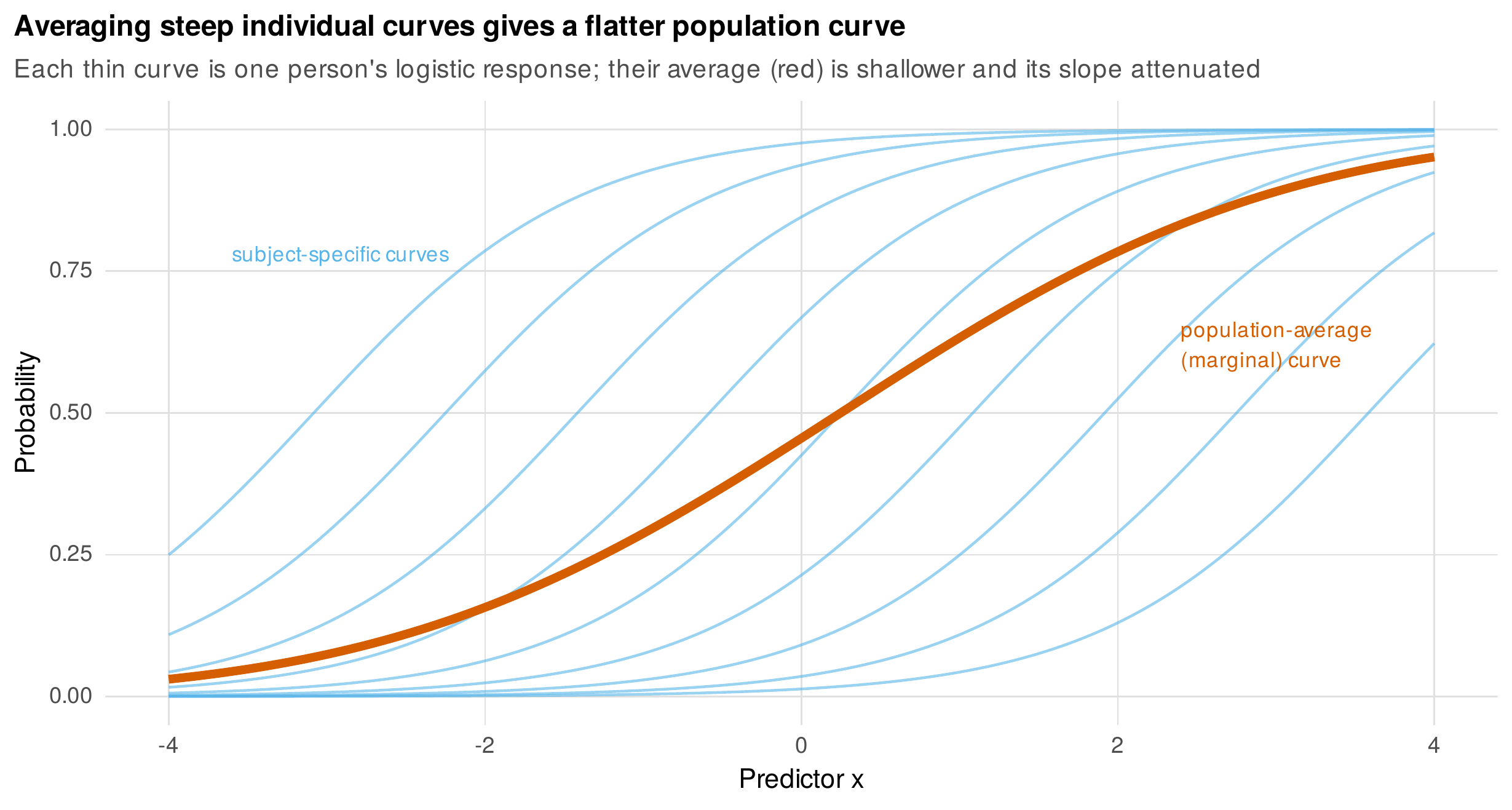
Note. Each thin curve is one person’s logistic probability of an outcome as a function of a predictor, the curves differing only in a random intercept. Their average across the population, the marginal curve in red, is shallower than any individual curve. The population-average slope is thus attenuated relative to the subject-specific slope; the two estimands differ for nonlinear links.
The attenuation is quantifiable. For a logistic model with a random intercept of variance \(\sigma_u^2\), the population-average slope is approximately the subject-specific slope divided by \(\sqrt{1 + c^2\sigma_u^2}\), where \(c = 16\sqrt{3}/(15\pi) \approx 0.588\) arises from approximating the logistic by a probit. Figure 12.2 confirms the relation by simulation: the ratio of the population-average to the subject-specific slope, estimated by fitting both models to data generated with a known random-intercept variance, tracks the formula closely and falls steadily as the between-person variance grows, from equality when everyone shares the same intercept to roughly one-half when the between-person variance is large. The practical consequence is that a logistic regression coefficient means different things depending on which model produced it, and the two must not be compared or pooled as though they were the same quantity. Table 12.1 states the distinction, and the mapping to research questions is the section’s payload: program evaluation, epidemiological, and policy questions, which concern what happens to a population, call for the population-average estimand, whereas questions about individual process and mechanism, which concern what happens within a person, call for the subject-specific one.
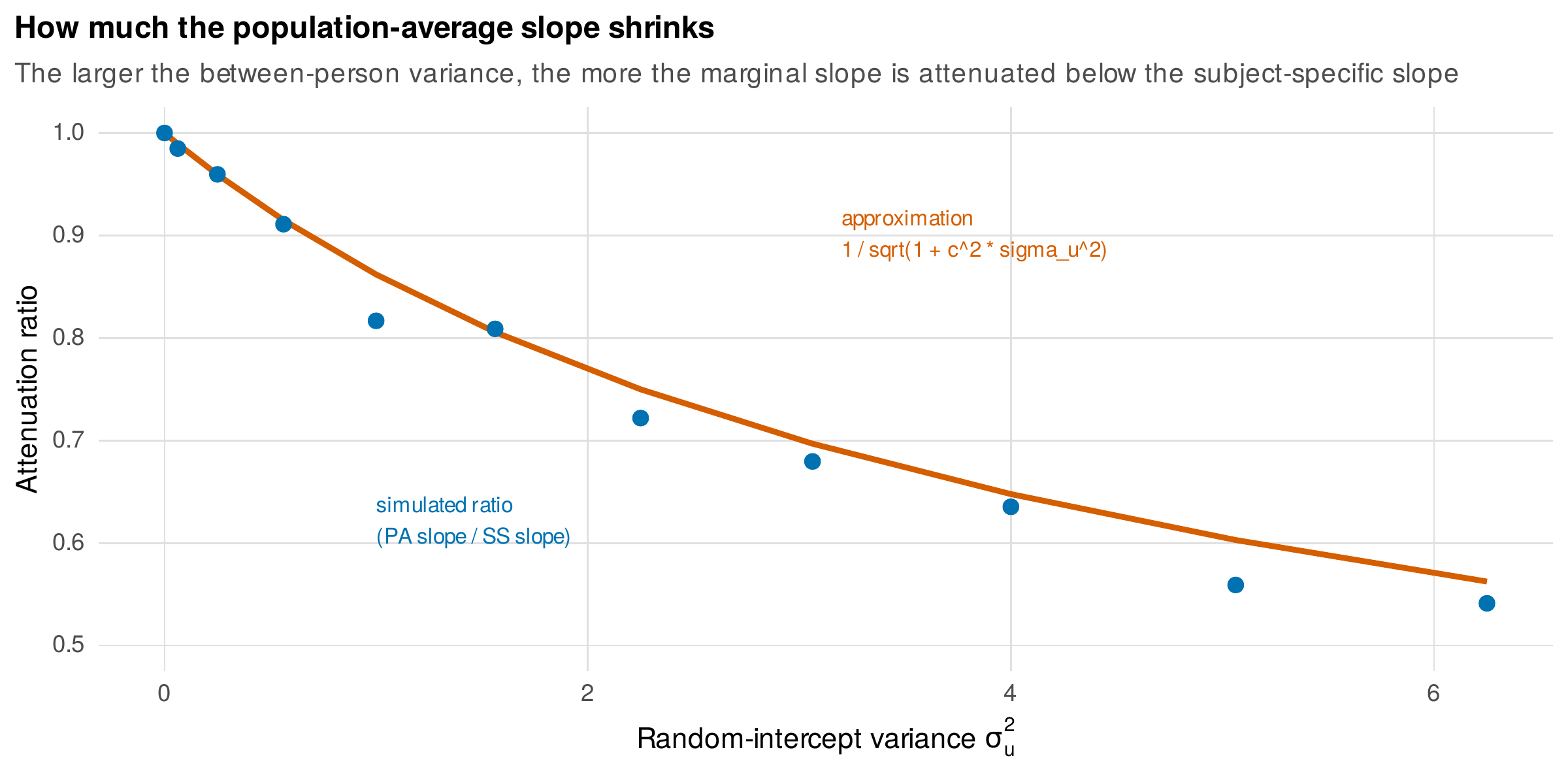
Note. The ratio of the population-average to the subject-specific logistic slope, from simulation (points), against the random-intercept variance, with the approximation \(1/\sqrt{1 + c^2\sigma_u^2}\) (curve). The larger the between-person variance, the more the marginal slope is attenuated below the subject-specific slope. The two coincide only when there is no between-person variation.
Table 12.1. Marginal versus conditional estimands.
| Feature | Population-average (marginal) | Subject-specific (conditional) |
|---|---|---|
| Question | How does the population average change? | How does an individual change? |
| Model | GEE | Mixed model (GLMM) |
| Coincide when | Identity link, or no between-person variance | |
| Diverge when | Nonlinear link (e.g., logistic): marginal slope attenuated | |
| Typical use | Program evaluation, policy, epidemiology | Process, mechanism, individual differences |
Note. Neither estimand is more correct; they answer different questions. The error is to fit one and interpret it as the other, which for logistic models means reading an attenuated population-average coefficient as an individual effect.
12.2 The Machinery of Generalized Estimating Equations
A generalized estimating equation is specified in three independent pieces (Liang & Zeger, 1986). A mean model links a function of the average outcome to the predictors, exactly as in an ordinary generalized linear model, so that for the binary remission outcome of the therapy trial a logistic mean model expresses the log-odds of remission as a function of arm and week. A variance function states how the variance of the outcome depends on its mean, again as in a generalized linear model. And a working correlation \(R(\alpha)\) describes the within-person dependence among the repeated measurements, the piece an ordinary generalized linear model lacks. Figure 12.3 shows the standard choices: independence, which ignores the within-person correlation; exchangeable, which assumes a single common correlation between any two occasions; autoregressive, which lets the correlation decay with the separation in time; and unstructured, which estimates every pairwise correlation freely. The remarkable and defining property of the method, derived in the Foundations box, is that the estimate of the mean-model coefficients is consistent even when the working correlation is wrong, because the estimating equation for the mean is unbiased regardless of the assumed dependence. The working correlation affects only efficiency, not validity, which is why it is called “working”: it is a device to improve precision, not an assumption the conclusions rest on. This is confirmed empirically in the therapy trial, where the estimated arm-by-week effect on remission is essentially the same, near \(0.14\) on the log-odds scale, whether independence, exchangeable, or autoregressive correlation is assumed, while the standard errors differ slightly. Table 12.2 guides the choice by design.
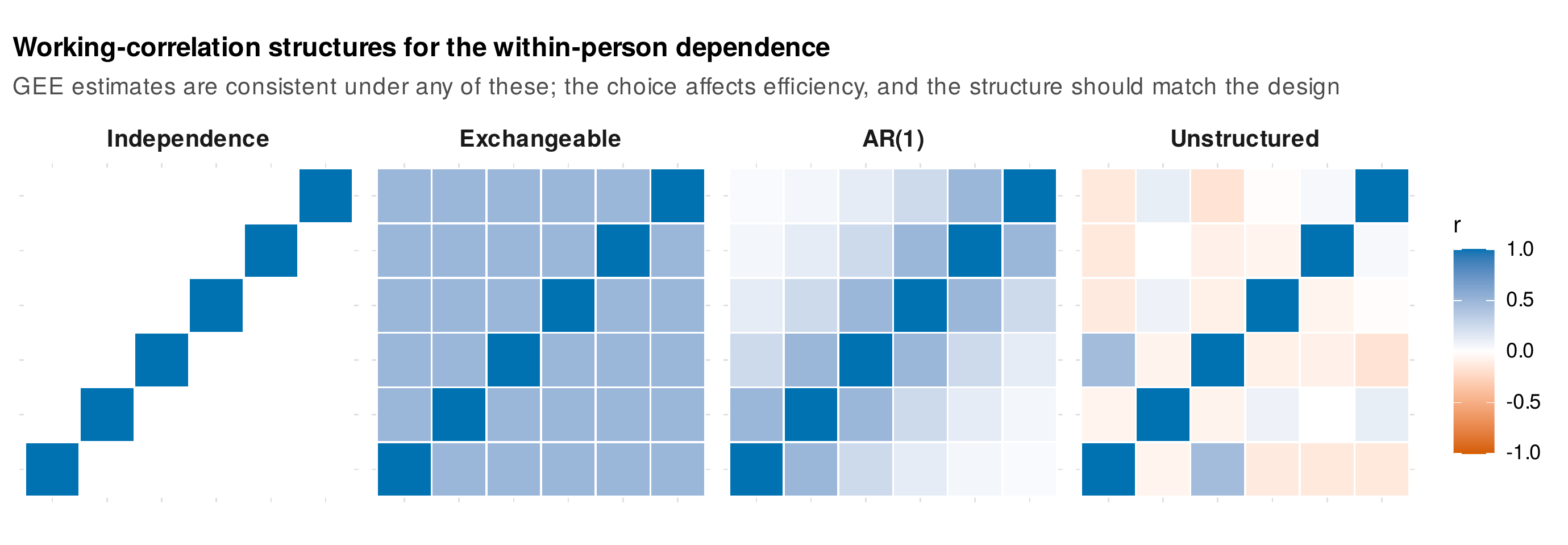
Note. Four working-correlation structures as heatmaps: independence (no within-person correlation), exchangeable (one common correlation), autoregressive (decaying with time separation), and unstructured (every pair free). The coefficient estimates are consistent under any of these; the choice affects only efficiency, and the structure should match the design.
Foundations Box • Estimating equations and the sandwich variance
An ordinary generalized linear model estimates \(\beta\) by solving the score equation \(\sum_i D_i^\top V_i^{-1} (y_i - \mu_i) = 0\), where for person \(i\) the vector \(y_i\) collects the repeated outcomes, \(\mu_i\) their modeled means, \(D_i = \partial\mu_i/\partial\beta\), and \(V_i\) a covariance. A generalized estimating equation uses the same form but builds \(V_i = A_i^{1/2} R(\alpha) A_i^{1/2}\) from the variance function \(A_i\) and the working correlation \(R(\alpha)\). Because \(E[y_i - \mu_i] = 0\) whenever the mean model is correct, the estimating equation has expectation zero regardless of whether \(R(\alpha)\) is the true correlation, so \(\hat\beta\) is consistent even under a misspecified working correlation. The price is that the model-based variance, which assumes \(V_i\) is correct, is then wrong, so inference uses the sandwich (robust) estimator \(\hat{\mathrm{Var}}(\hat\beta) = B^{-1} M B^{-1}\), with \(B = \sum_i D_i^\top V_i^{-1} D_i\) the “bread” and \(M = \sum_i D_i^\top V_i^{-1} \hat{e}_i \hat{e}_i^\top V_i^{-1} D_i\) the “meat” built from the empirical residuals \(\hat{e}_i = y_i - \hat\mu_i\). The meat estimates the true residual covariance from the data, which is why the sandwich is robust to a wrong working correlation, and why it needs enough clusters to estimate that covariance well.
The robustness of the sandwich estimator is not free, and its cost is a small-sample fragility: the meat of the sandwich is an average of residual products across clusters, and when the number of clusters is small that average is a poor and downward-biased estimate of the true variance, so the standard errors are too small and confidence intervals too narrow. Figure 12.4 shows the consequence in a coverage simulation: with a hundred clusters the ninety-five-percent interval covers at nearly its nominal rate, but with ten or fifteen clusters it covers only ninety-two percent of the time, an inflation of the true error rate that would make many published small-sample generalized-estimating-equation analyses anticonservative. The remedies are the bias-corrected sandwich estimators, which adjust the residuals to remove the downward bias, and the practical guidance is to apply such a correction whenever the number of clusters is below roughly forty to fifty (Mancl & DeRouen, 2001; Kauermann & Carroll, 2001). Table 12.3 lists the corrections and when each is required.
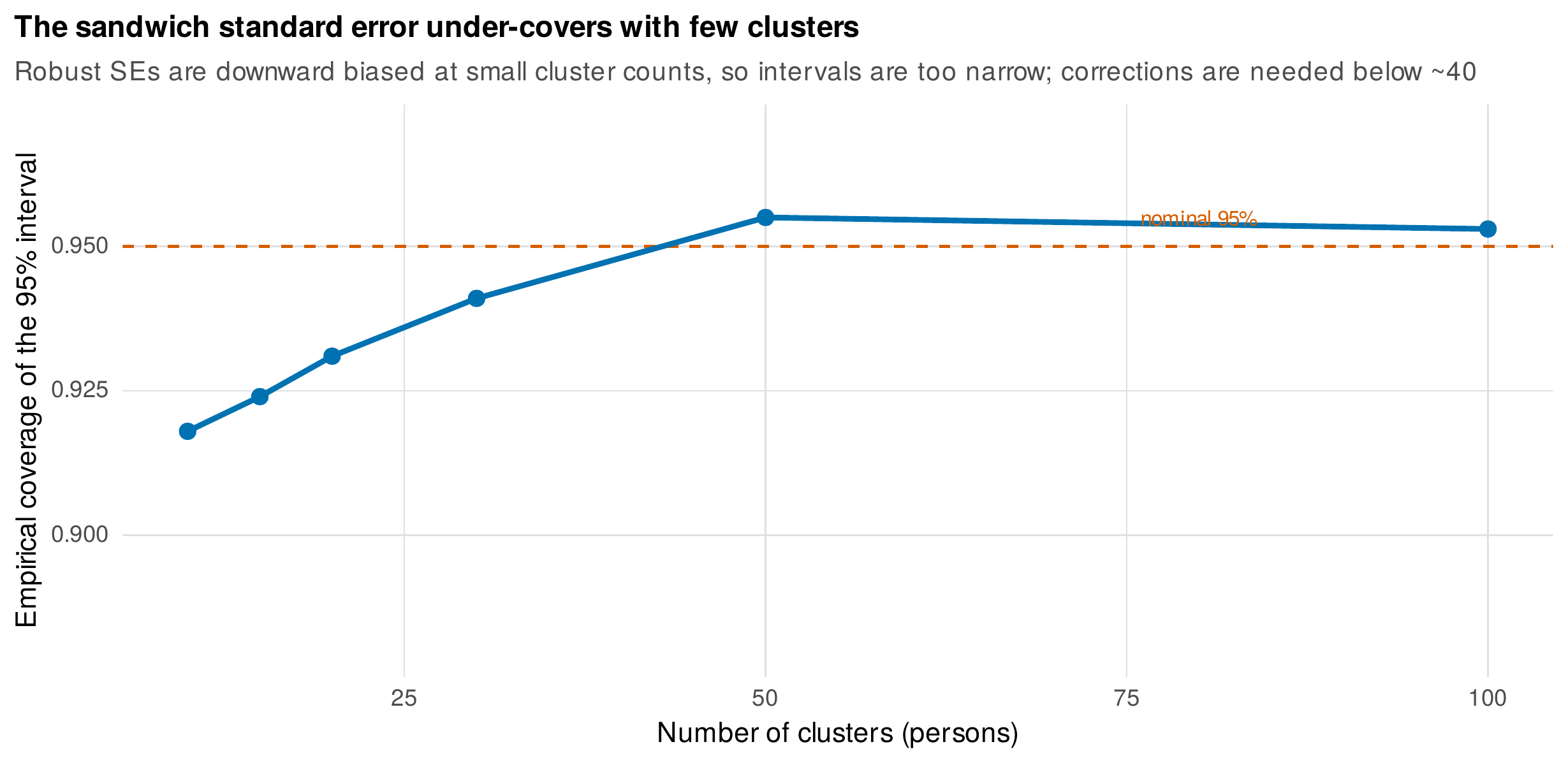
Note. Empirical coverage of the nominal ninety-five-percent confidence interval for a time slope, from a simulation, against the number of clusters. With few clusters the robust standard error is downward biased and the interval covers below its nominal rate; the shortfall is negligible by about fifty clusters. Small-sample corrections are needed below roughly forty.
Table 12.2. Working-correlation selection by design.
| Structure | Plausible when | Note |
|---|---|---|
| Independence | Interest only in the mean; robustness paramount | Consistent; least efficient; sandwich SE essential |
| Exchangeable | Few waves, no natural time ordering | One correlation parameter |
| Autoregressive | Equally spaced waves with decaying dependence | Matches longitudinal structure |
| Unstructured | Few waves, many persons | Many parameters; unstable at long series |
Note. Because the coefficient estimates are consistent under any structure, the choice is about efficiency and, for the unstructured form, feasibility. Exchangeable is a poor default for longitudinal data, whose correlations decay with time.
Table 12.3. Robust standard-error corrections.
| Estimator | What it does | When required |
|---|---|---|
| Naive sandwich | Empirical residual covariance | Many clusters (\(> 40\)–\(50\)) |
| Mancl-DeRouen | Inflates residuals to remove bias | Few clusters |
| Kauermann-Carroll | Alternative bias correction | Few clusters |
| Cluster-robust CR2 | Bias-reduced cluster-robust variance | Few clusters; small-sample \(t\) reference |
Note. All target the same problem, that the naive sandwich underestimates variance when clusters are few. With adequate clusters the corrections converge on the naive estimator, so applying one is rarely harmful.
12.3 Model Evaluation and Selection
Because a generalized estimating equation is not fitted by maximizing a likelihood, the familiar likelihood-based tools are unavailable, and their closest replacement is the quasi-likelihood information criterion (QIC) of Pan (2001), which adapts the Akaike criterion to the quasi-likelihood setting and can be used to compare working-correlation structures and, in a variant, mean models. The criterion must be used judiciously and never worshipped, because it is not a true likelihood and its behavior is less well understood than the Akaike criterion it imitates; it is a rough guide to the working correlation, not an arbiter of substantive models. The absence of a likelihood also means there is no natural coefficient of determination, and the honest way to communicate a generalized-estimating-equation fit is through predicted quantities on the scale of interest, the population-average probabilities or means implied by the model, rather than through a summary statistic that the method does not naturally provide.
12.4 Missing Data: The Method’s Soft Spot
The generalized estimating equation carries a liability that is easy to overlook and directly opposed to a common misconception. Because it makes no full distributional assumption, it is often supposed to handle missing data gracefully, but the truth is the reverse: the unweighted estimating equation is valid only when the data are missing completely at random, a far stronger requirement than the missing-at-random condition under which the likelihood methods of Chapter 6 remain valid. Under the missing-at-random dropout typical of longitudinal studies, where those doing worse are more likely to leave, the unweighted method is biased, because it effectively averages over the selected sample of those who remain. Figure 12.5 is the chapter’s signature exhibit, a known-truth simulation in which a symptom declines over time and dropout depends on the previous observed value, so that sicker patients leave and the survivors are systematically healthier. The unweighted generalized estimating equation, tracking the observed survivors, reports a mean trajectory that falls well below the truth and so overstates improvement, whereas the mixed model estimated by full-information maximum likelihood recovers the true trajectory almost exactly, because likelihood is valid under missing-at-random. The remedy within the marginal framework is the inverse-probability-weighted generalized estimating equation (Robins et al., 1995), which weights each observed record by the inverse of its estimated probability of still being in the study, upweighting the kinds of people who tend to drop out so that the observed sample is made to represent the full population. Figure 12.5 shows that this weighting repairs part of the bias, but only part, and the reason is instructive: the weighting uses only the marginal observed data, discarding the within-person information about where a departed person’s trajectory was heading that the likelihood method exploits in full. The exhibit therefore delivers two lessons at once, that the marginal method is fragile under realistic missingness, and that even its remedy is dominated by the likelihood approach that the rest of the book favors.
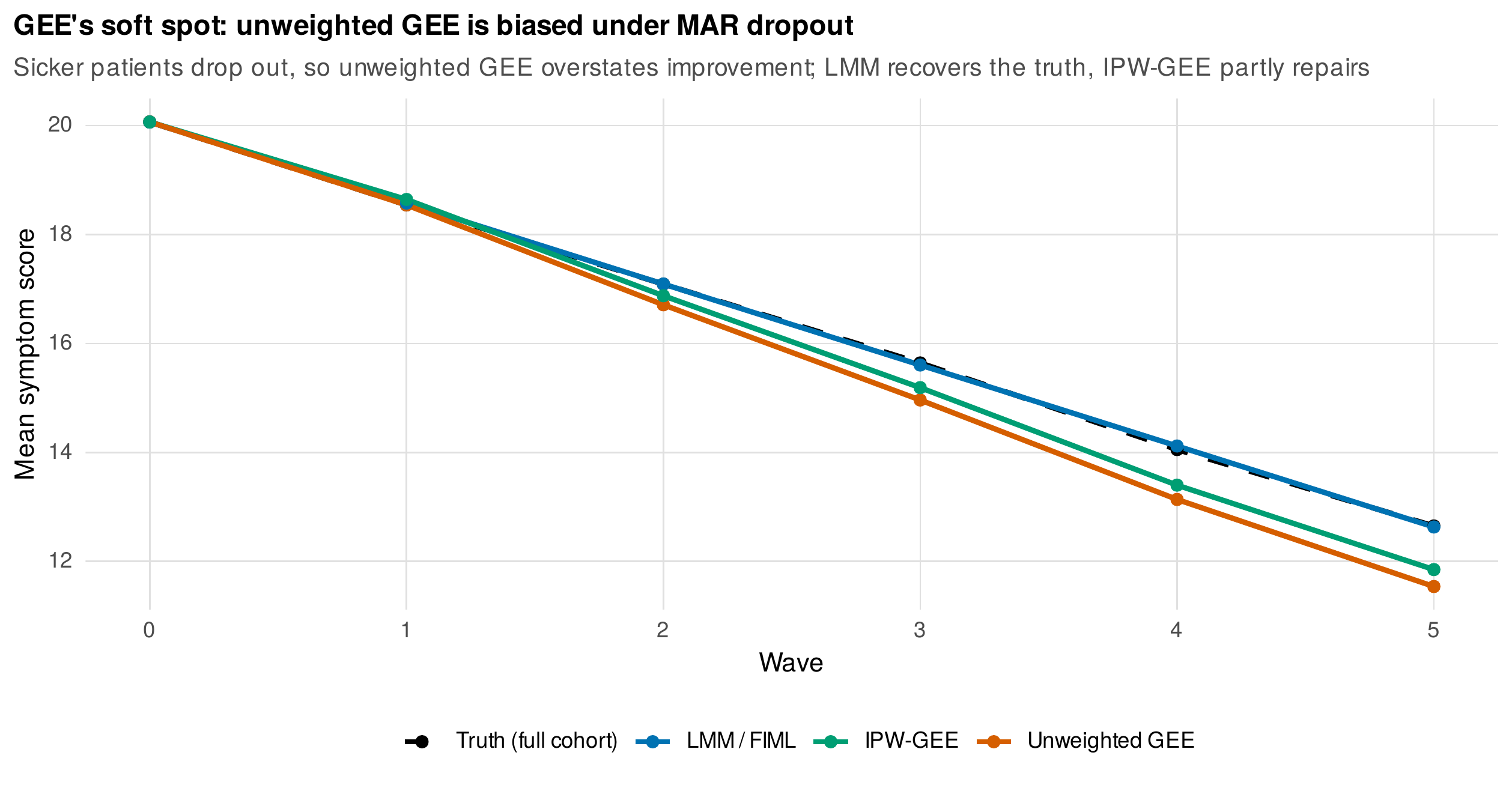
Note. A known-truth simulation in which a symptom declines and sicker patients drop out (missing at random, depending on the previous observed value). The unweighted generalized estimating equation (orange) falls below the true cohort mean (dashed) and overstates improvement; the mixed model by maximum likelihood (blue) recovers the truth; the inverse-probability-weighted estimating equation (green) repairs part of the bias but not all, because it discards the within-person information likelihood uses.
12.5 Generalized Estimating Equations in Practice
The primary worked example fits the population-average probability of remission in the therapy trial as a function of arm and week. The model reports how the average remission rate in each arm evolves, and Figure 12.6 displays those model-implied population-average probabilities: both arms improve, and the treatment arm’s remission probability rises faster, the arm-by-week interaction being the population-average treatment effect. This is exactly the quantity a program evaluation wants, the change in the population rate, and it is reported as a probability rather than as a log-odds coefficient precisely because the population-average probability is interpretable while the attenuated coefficient invites the subject-specific misreading warned against above. A second example, a day-level binary outcome in the experience-sampling data modeled on within-person predictors, would illustrate the honest limit of the approach: when the interest is genuinely in the within-person process, whether a person is more likely to act a certain way on days when they are more stressed than usual, the population-average estimand answers a subtly different question, and the subject-specific mixed model of Chapters 15 and 23 is the better tool. Table 12.4 is the reporting checklist.
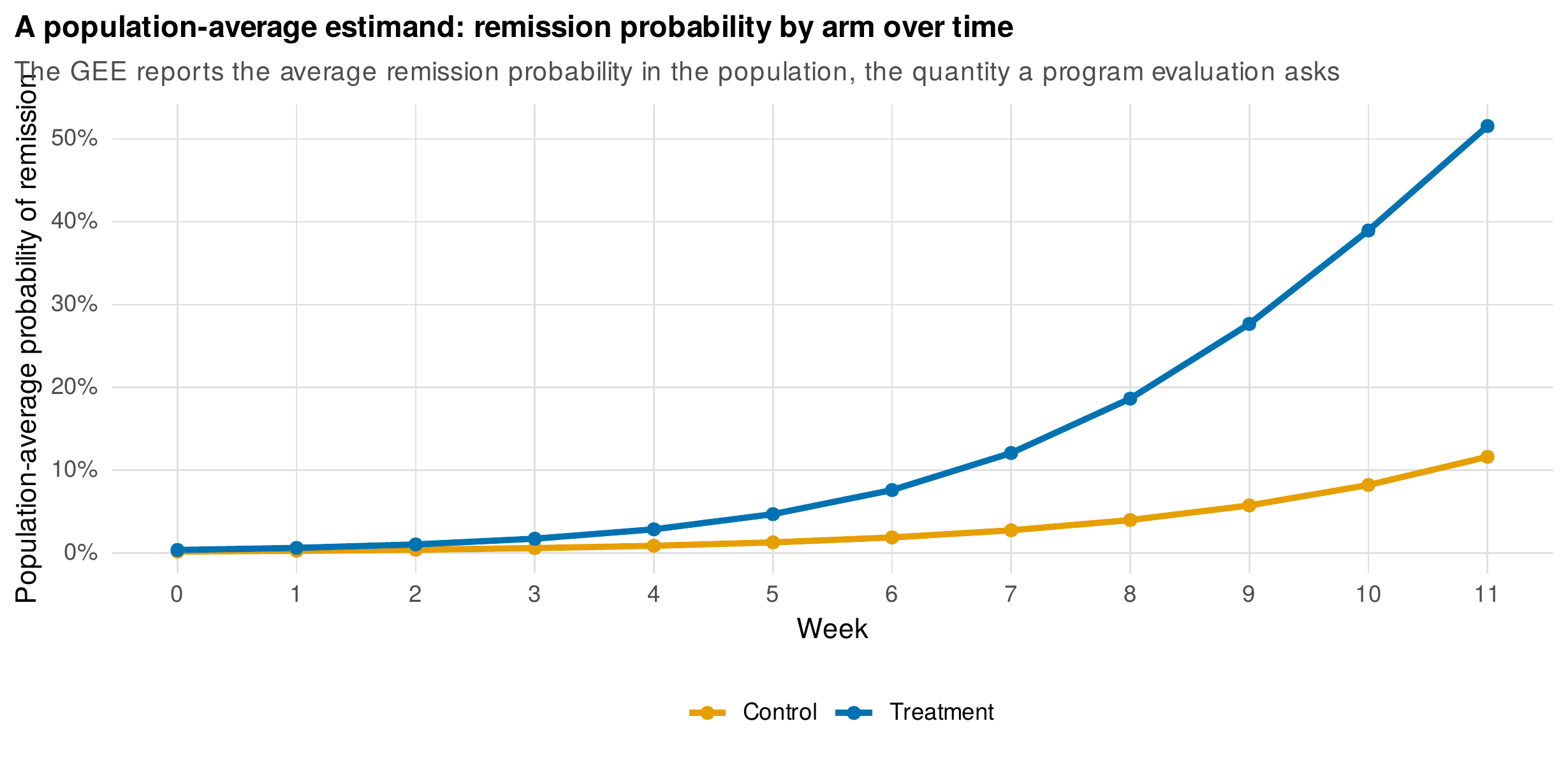
Note. Model-implied population-average probability of remission in the therapy trial for each arm across weeks, from a logistic generalized estimating equation. Both arms improve and the treatment arm improves faster; the arm-by-week difference is the population-average treatment effect, the quantity a program evaluation asks about.
Table 12.4. Reporting checklist for generalized estimating equations.
| Element | What to report |
|---|---|
| Estimand | That the estimand is population-average, stated explicitly |
| Model | Mean model and link; variance function; working correlation |
| Standard errors | Robust (sandwich); which small-sample correction, if any, and the cluster count |
| Missingness | The missing-completely-at-random assumption, or the weighting used to relax it |
| Interpretation | Effects on the scale of interest (probabilities or means), not raw coefficients |
Note. The single most important line is the first: naming the estimand as population-average prevents the reader from misinterpreting an attenuated logistic coefficient as a subject-specific effect.
12.6 Choosing Between Marginal and Mixed Models
The choice between a generalized estimating equation and a mixed model is not a matter of statistical taste but of estimand and assumptions, and Figure 12.7 lays out the decision. The first and governing question is which estimand the research wants: a population-average answer points to the marginal model, a subject-specific answer to the mixed model, and for a linear outcome the two coincide so either will do. The second question is the missingness mechanism: data missing at random, the common case, are handled validly by the likelihood-based mixed model but require weighting for the marginal model. The third concerns what the analysis must deliver: only the mixed model provides estimates of the random-effect variances, the individual differences in change that are often the substantive quantity of interest, and their absence from the marginal model is both a simplification and a genuine loss. The remaining considerations, the number of clusters and computational robustness, favor the marginal model when clusters are few and the mixed model’s random-effect structure is hard to estimate. Table 12.5 summarizes the comparison. The two methods are coordinated, not opposed: the generalized linear mixed model of Chapter 15 is the subject-specific counterpart of the marginal model developed here, and the attenuation relation of Section 12.1 is exactly the bridge between their coefficients.
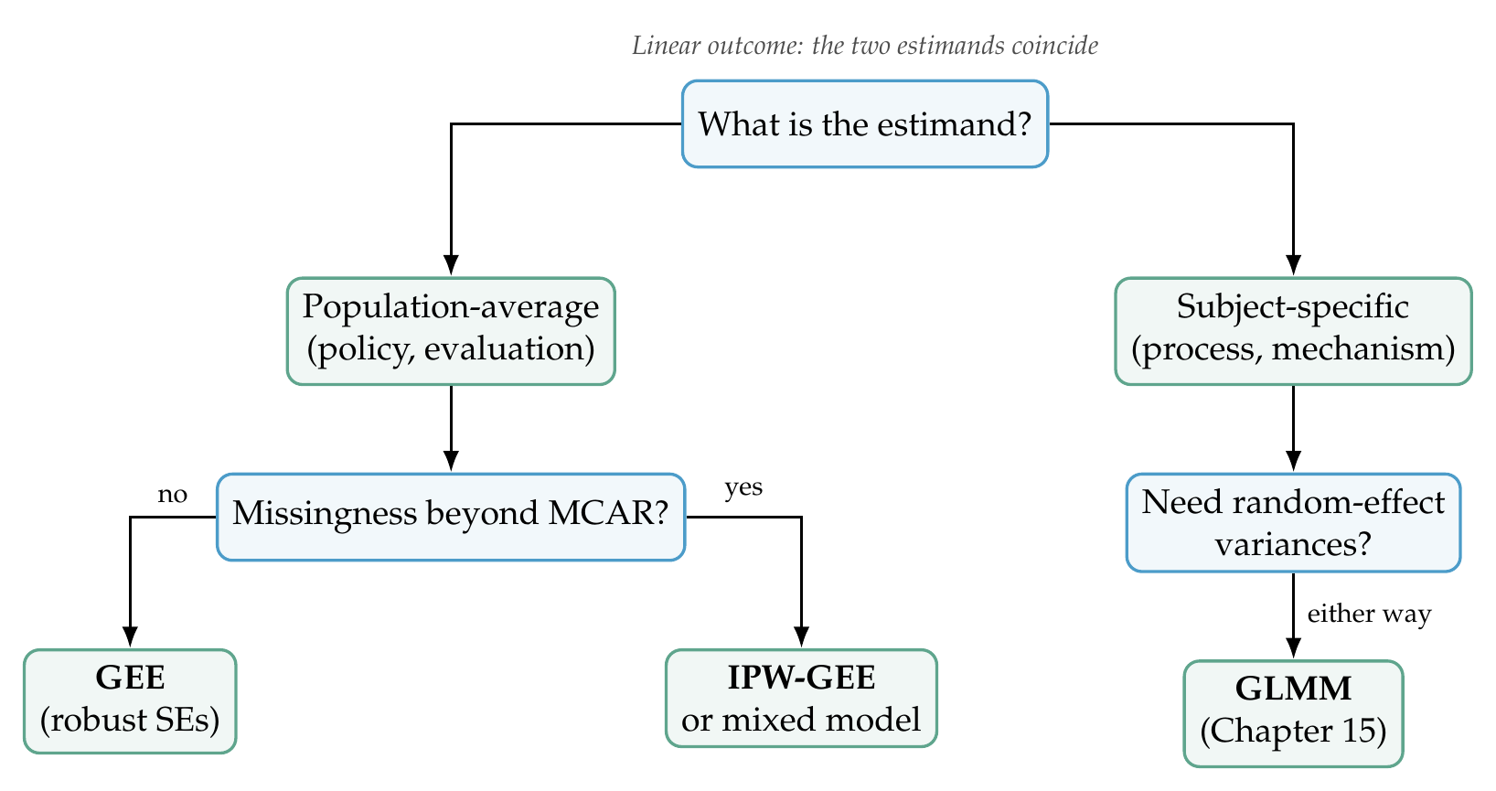
Note. The estimand governs the choice: a population-average question leads to the generalized estimating equation, a subject-specific question to the generalized linear mixed model. Missingness beyond missing-completely-at-random requires weighting or a likelihood method; the need for random-effect variances requires the mixed model. For a linear outcome the two estimands coincide.
Table 12.5. Generalized estimating equations versus mixed models.
| Feature | GEE (marginal) | Mixed model (conditional) |
|---|---|---|
| Estimand | Population-average | Subject-specific |
| Missing data valid under | MCAR (MAR with weighting) | MAR (by likelihood) |
| Random-effect variances | Not estimated | Estimated |
| Dependence | Working correlation (nuisance) | Modeled by random effects |
| Small clusters | Robust; needs SE correction | Random-effect variance hard to estimate |
| Nonlinear link coefficients | Attenuated (marginal) | Larger (conditional) |
Note. The methods answer different questions and are valid under different missingness assumptions. The choice is dictated by the estimand and the missingness mechanism, not by a preference for one statistical tradition.
12.7 Running Generalized Estimating Equations in R
The geepack package fits generalized estimating equations, taking the cluster identifier through its id argument and the working correlation through corstr, and reporting robust standard errors by default. The population-average remission model and the comparison across working correlations are a few lines.
library(geepack); library(dplyr)
rct <- readRDS("Examples/data/therapy_rct.rds") |>
  mutate(arm = factor(arm, levels = c("Control","Treatment")),
         remit = as.integer(hdrs <= 7)) |>
  filter(!is.na(hdrs)) |> arrange(patient_id, week)

# --- Population-average logistic model; robust SEs are the default ---
fit <- geeglm(remit ~ week * arm, id = patient_id, data = rct,
              family = binomial, corstr = "exchangeable")
summary(fit)                                   # week:armTreatment is the PA effect

# --- Coefficients are consistent across working correlations ---
sapply(c("independence","exchangeable","ar1"), function(cs)
  coef(geeglm(remit ~ week * arm, id = patient_id, data = rct,
              family = binomial, corstr = cs))["week:armTreatment"])
The population-average probabilities for the margins plot come from predict on the fitted model, and the inverse-probability-weighted analysis passes weights to the same fitting function. The complete code, including the attenuation and coverage simulations and the missing-at-random fragility exhibit with its cumulative dropout weights, is the shipped script ch12_analysis_V01.R, with figures drawn by ch12_figures_V01.R.
# --- Population-average predicted probabilities by arm and week ---
newd <- expand.grid(week = 0:11, arm = factor(c("Control","Treatment")))
newd$p <- predict(fit, newdata = newd, type = "response")

# --- Inverse-probability weighting to relax MCAR toward MAR ---
# weights w = 1 / (cumulative probability of remaining), from a dropout model;
# pass to geeglm and use an independence working correlation
gee_ipw <- geeglm(y ~ factor(t), id = id, data = observed, weights = w,
                  corstr = "independence")
Software Note • which GEE package, and cross-reading other software
Three R packages fit generalized estimating equations, with small but real differences. The geepack package (Halekoh et al., 2006), used here, offers a clean formula interface, several working correlations, and an anova method for Wald tests of nested mean models; it is the recommended default. The older gee package reports both naive and robust standard errors side by side, which is pedagogically useful, but its interface is more dated. The geeM package is built for speed on large data. Small-sample sandwich corrections are available through geesmv and the cluster-robust clubSandwich package, the latter providing the bias-reduced CR2 estimator with a small-sample \(t\) reference distribution. Readers cross-reading from other environments will find the same models under xtgee in Stata and PROC GENMOD with a REPEATED statement in SAS; the estimand and the robust standard errors are identical across all of them.
12.8 Interpreting and Reporting the Results
A generalized-estimating-equation result is reported by naming the estimand, describing the three model pieces, and interpreting effects on the scale of interest. A model paragraph for the therapy trial reads: “The population-average probability of remission was modeled with a logistic generalized estimating equation with an exchangeable working correlation and robust standard errors, treating patients as clusters (\(N = 240\)). The arm-by-week interaction, the population-average treatment effect, was positive on the log-odds scale (\(\hat\beta = 0.13\), robust \(SE = 0.09\)), and the model-implied population-average remission probability rose faster in the treatment arm, reaching a higher rate by week 12 (Figure 12.6). Estimates were essentially unchanged across independence, exchangeable, and autoregressive working correlations, as expected given the consistency of the coefficients. Because dropout was plausibly missing at random rather than completely at random, the primary inference relied on the mixed model of Chapter 13, with the generalized estimating equation reported as the population-average complement.” The estimand is named, the robust standard errors and working correlation are stated, and the missingness caveat is honest.
Common Pitfall • three errors with generalized estimating equations
First, reading a logistic coefficient as a person-specific effect: a population-average logistic coefficient is attenuated relative to the subject-specific one (Figure 12.1), so interpreting it as the effect for an individual understates the within-person association; report the estimand and, if the individual effect is wanted, fit a mixed model. Second, worshipping the quasi-likelihood criterion: the criterion is a rough guide to the working correlation, not a substantive model-selection oracle, and it does not license the comparisons a true likelihood would. Third, independence working correlation with few clusters and naive standard errors: this combination is doubly fragile, forfeiting efficiency and relying on a sandwich estimator that under-covers at small cluster counts (Figure 12.4); use a plausible working correlation and a small-sample correction.
12.9 Common Misconceptions
Several beliefs about generalized estimating equations mislead. The first is that a generalized estimating equation is just a mixed model fitted by different software; the two answer different questions, the marginal and the conditional, which for nonlinear links are different quantities, and are valid under different missingness assumptions. The second is that robust standard errors fix everything; the sandwich estimator protects against a misspecified working correlation but not against a misspecified mean model, and it is itself fragile when clusters are few. The third is that exchangeable correlation is a safe default for longitudinal data; longitudinal correlations decay with time, so an autoregressive structure is usually more plausible, though the choice affects only efficiency. The fourth, and the most consequential, is that the method handles missing data well because it makes no distributional assumptions; the reverse is true, as the unweighted method requires the strong missing-completely-at-random condition and is biased under the missing-at-random dropout that likelihood methods handle. A recurring question, why a reviewer might demand one method or the other, is answered by returning to the estimand: name the quantity the study is about, and the method follows.
Chapter Summary
A single regression can answer two different questions, the population-average and the subject-specific, and for nonlinear links they diverge: the marginal logistic slope is attenuated relative to the conditional one by a factor that grows with the between-person variance (Figures 12.1, 12.2). Generalized estimating equations target the population-average estimand through a mean model, a variance function, and a working correlation, and their defining property is that the coefficient estimates are consistent even when the working correlation is wrong (Figure 12.3), so the working structure affects efficiency, not validity. Inference uses the robust sandwich standard error, which is fragile at small cluster counts and under-covers below roughly forty clusters unless a small-sample correction is applied (Figure 12.4). The method’s chief liability is missing data: the unweighted estimating equation requires data missing completely at random and is biased under the missing-at-random dropout that likelihood methods handle validly, a fragility that inverse-probability weighting only partly repairs (Figure 12.5). Population-average effects are reported on the scale of interest as probabilities or means (Figure 12.6), and the choice between the marginal and mixed-model approaches is dictated by estimand and missingness rather than by taste (Figure 12.7), with the generalized linear mixed model of Chapter 15 as the subject-specific counterpart of the method developed here.
Where to Go Next
The marginal model is one of two roads out of the classical methods, and the mixed model is the other, developed across Part IV. Chapter 13 introduces the linear mixed model whose random intercept and slope restore the individual differences the marginal model omits, and whose likelihood estimation is valid under missing at random; the robust standard errors learned here reappear there as an option for clustered inference. Chapter 15 completes the pair begun in this chapter, developing the generalized linear mixed model as the subject-specific counterpart to the marginal model, where the attenuation relation of Section 12.1 becomes the explicit translation between the two sets of coefficients. The inverse-probability-weighting logic returns in the survival models of Chapter 29, and the estimand-first discipline, naming the quantity before choosing the model, recurs wherever a causal or descriptive target must be made precise, most pointedly in the cross-lagged panel debates of Chapter 21. The lesson carried forward is that the question chooses the estimand, the estimand chooses the model, and no amount of robustness substitutes for asking the question correctly.
Exercises
- 12.1 Verify the attenuation. Simulate person-specific logistic data with a known random-intercept variance, fit both a generalized linear mixed model and a generalized estimating equation, and confirm that the ratio of their slopes matches the attenuation formula.
- 12.2 Working correlations. Refit the remission example under independence, exchangeable, and autoregressive working correlations, and report how the coefficient and its robust standard error change; explain the stability of the coefficient.
- 12.3 Build the fragility. Construct a missing-at-random dropout mechanism on a simulated dataset, show the bias of the unweighted generalized estimating equation against the mixed model, and repair it with inverse-probability weighting.
- 12.4 Small-cluster coverage. Simulate a study with fifteen clusters and estimate the empirical coverage of the naive and a bias-corrected sandwich standard error.
- 12.5 Estimand essay. For three research vignettes, decide whether the population-average or the subject-specific estimand is wanted, and defend each choice in a short paragraph.
References
Fitzmaurice, G. M., Laird, N. M., & Ware, J. H. (2011). Applied longitudinal analysis (2nd ed.). Wiley.
Gardiner, J. C., Luo, Z., & Roman, L. A. (2009). Fixed effects, random effects and GEE: What are the differences? Statistics in Medicine, 28(2), 221–239. https://doi.org/10.1002/sim.3478
Halekoh, U., Højsgaard, S., & Yan, J. (2006). The R package geepack for generalized estimating equations. Journal of Statistical Software, 15(2), 1–11. https://doi.org/10.18637/jss.v015.i02
Hardin, J. W., & Hilbe, J. M. (2013). Generalized estimating equations (2nd ed.). Chapman and Hall/CRC.
Hubbard, A. E., Ahern, J., Fleischer, N. L., Van der Laan, M., Lippman, S. A., Jewell, N., Bruckner, T., & Satariano, W. A. (2010). To GEE or not to GEE: Comparing population average and mixed models for estimating the associations between neighborhood risk factors and health. Epidemiology, 21(4), 467–474. https://doi.org/10.1097/EDE.0b013e3181caeb90
Kauermann, G., & Carroll, R. J. (2001). A note on the efficiency of sandwich covariance matrix estimation. Journal of the American Statistical Association, 96(456), 1387–1396. https://doi.org/10.1198/016214501753382309
Liang, K.-Y., & Zeger, S. L. (1986). Longitudinal data analysis using generalized linear models. Biometrika, 73(1), 13–22. https://doi.org/10.1093/biomet/73.1.13
Mancl, L. A., & DeRouen, T. A. (2001). A covariance estimator for GEE with improved small-sample properties. Biometrics, 57(1), 126–134. https://doi.org/10.1111/j.0006-341X.2001.00126.x
McNeish, D., Stapleton, L. M., & Silverman, R. D. (2017). On the unnecessary ubiquity of hierarchical linear modeling. Psychological Methods, 22(1), 114–140. https://doi.org/10.1037/met0000078
Pan, W. (2001). Akaike’s information criterion in generalized estimating equations. Biometrics, 57(1), 120–125. https://doi.org/10.1111/j.0006-341X.2001.00120.x
Robins, J. M., Rotnitzky, A., & Zhao, L. P. (1995). Analysis of semiparametric regression models for repeated outcomes in the presence of missing data. Journal of the American Statistical Association, 90(429), 106–121. https://doi.org/10.1080/01621459.1995.10476493
Zeger, S. L., & Liang, K.-Y. (1986). Longitudinal data analysis for discrete and continuous outcomes. Biometrics, 42(1), 121–130. https://doi.org/10.2307/2531248
Zeger, S. L., Liang, K.-Y., & Albert, P. S. (1988). Models for longitudinal data: A generalized estimating equation approach. Biometrics, 44(4), 1049–1060. https://doi.org/10.2307/2531734