Chapter 13
Linear Mixed-Effects Models: Foundations
This is the load-bearing chapter of the book. The mixed model it develops is the machinery on which the rest of Parts IV through VI is built, and the notation introduced here binds the chapters that follow. The repeated-measures analysis of variance of Chapter 11 was shown there to be a constrained special case of a more general model; this chapter is where the general model arrives, relaxing every one of those constraints at once. It admits individually varying and continuous time, unbalanced and incomplete data handled by likelihood rather than deletion, flexible covariance structures, and, most importantly, genuine individual differences in change through random slopes. Four things must be delivered with full rigor: the specification and interpretation of the model, the estimation and inference that turn data into parameters and uncertainty, the centering decision that determines what question a time-varying predictor answers, and a complete practical workflow for building, diagnosing, and reporting a mixed model. Each equation is followed by the plain-language paragraph that makes it usable, because a reader who leaves this chapter fluent will read the rest of the book with ease.
Learning Objectives
After working through this chapter, you should be able to: (1) write the two-level linear mixed model in both hierarchical and combined form and translate between them; (2) interpret the fixed effects, the random-effect variances and their covariance, and the residual variance substantively; (3) explain shrinkage and the best linear unbiased predictions of individual effects; (4) distinguish maximum likelihood from restricted maximum likelihood and use each appropriately; (5) conduct inference on fixed effects with a degrees-of-freedom correction and on variance components with the boundary-corrected likelihood-ratio test; (6) decompose a time-varying predictor by person-mean centering and interpret its within-person, between-person, and contextual effects; and (7) build a model by a principled sequence, diagnose and troubleshoot it, quantify variance explained, and report it to publication standard.
13.1 From Constrained to Flexible: The Model
The linear mixed model can be written in two equivalent forms, and fluency requires holding both. The hierarchical form separates the levels of the data explicitly. At level one, the within-person level, each person’s outcome on each occasion is a person-specific line plus residual noise, \(y_{it} = \beta_{0i} + \beta_{1i}x_{it} + e_{it}\), where \(\beta_{0i}\) and \(\beta_{1i}\) are person \(i\)’s own intercept and slope. At level two, the between-person level, each person’s coefficients are the population average plus a person-specific departure, \(\beta_{0i} = \gamma_{00} + u_{0i}\) and \(\beta_{1i} = \gamma_{10} + u_{1i}\). Substituting the second into the first yields the combined form, \(y_{it} = \gamma_{00} + \gamma_{10}x_{it} + u_{0i} + u_{1i}x_{it} + e_{it}\), which separates the fixed effects \(\gamma\), the population-average intercept and slope, from the random effects \(u\), the person-specific deviations, and the residual \(e\). The residuals are assumed \(e_{it} \sim N(0, \sigma^2)\) and the random effects are assumed to follow a bivariate normal distribution with mean zero and a covariance matrix, the T matrix, \(\mathbf{T} = \left(\begin{smallmatrix} \tau_{00} & \tau_{01} \\ \tau_{01} & \tau_{11} \end{smallmatrix}\right)\), whose diagonal holds the variance of intercepts and the variance of slopes and whose off-diagonal holds their covariance. Figure 13.1 builds the model up visually on the sleepstudy data, in which reaction time worsens over successive days of sleep deprivation: from the raw trajectories, to a model with random intercepts that lets people differ in overall level while sharing a slope, to the full model with random slopes that lets each person have their own rate of decline.
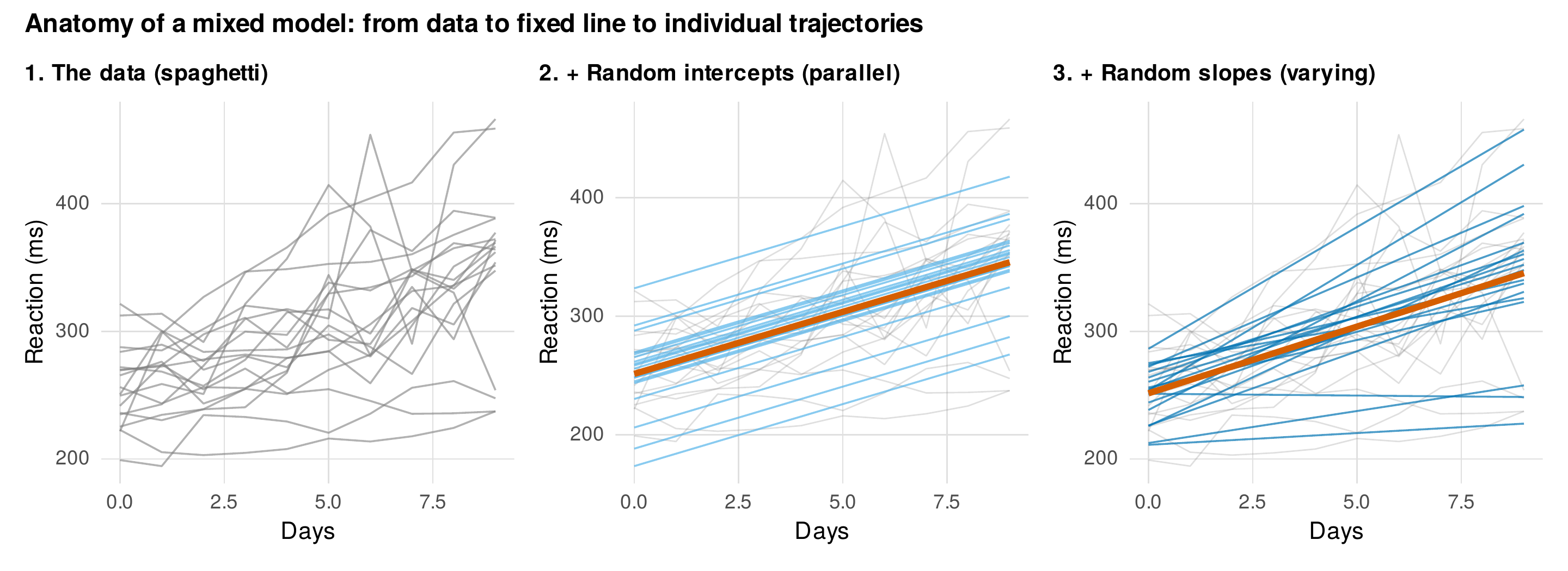
Note. The sleepstudy data (reaction time across days of sleep deprivation). Left: the raw trajectories. Middle: a random-intercept model, in which individual lines (blue) are parallel to the fixed line (red), differing only in level. Right: a random-slope model, in which the individual lines also differ in slope. The random effects are the departures of the blue lines from the red.
The variances and the covariance in the T matrix are not nuisance quantities but substantive descriptions of individual differences. The intercept variance \(\tau_{00}\) says how much people differ in their starting level, the slope variance \(\tau_{11}\) says how much they differ in their rate of change, and the intercept-slope covariance \(\tau_{01}\), usually read as a correlation, says whether people who start high change differently from people who start low. Figure 13.2 shows the two possibilities: a positive correlation produces a fan-spread, in which those who start higher also rise faster so that individual differences grow over time, and a negative correlation produces a fan-close, in which the trajectories converge. This correlation is often the substantive quantity of interest, telling whether inequality in an outcome widens or narrows with time, and it is estimated freely by the model rather than assumed.
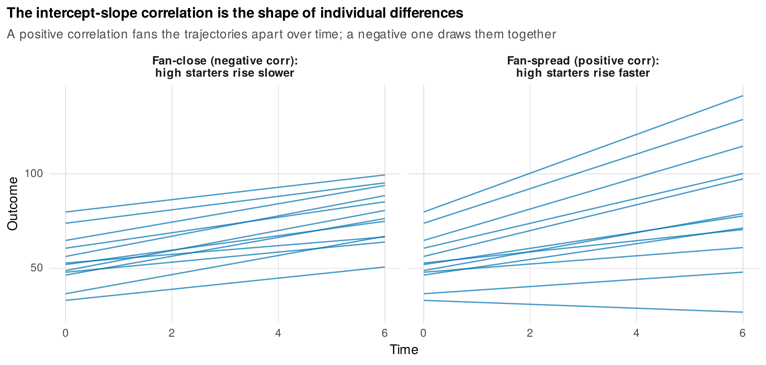
Note. Simulated trajectories under a positive intercept-slope correlation (left), where higher starters rise faster and the trajectories fan apart, and a negative correlation (right), where higher starters rise more slowly and the trajectories converge. The correlation, estimated in the T matrix, describes whether individual differences grow or shrink over time.
The random effects have a consequence that unifies this chapter with the two before it. Although the model is specified conditionally, in terms of person-specific lines, it implies a marginal covariance among the repeated measurements, obtained by integrating over the random effects: for person \(i\) with design matrix \(\mathbf{Z}_i\) for the random effects, the marginal covariance of the observations is \(\mathbf{Z}_i \mathbf{T} \mathbf{Z}_i' + \sigma^2 \mathbf{I}\). This single expression explains a great deal. A random-intercept-only model implies \(\mathbf{Z}_i \mathbf{T} \mathbf{Z}_i' + \sigma^2 \mathbf{I}\) with a constant off-diagonal, which is exactly the compound symmetry that Chapter 11’s repeated-measures analysis of variance assumed, so the random-intercept model is that analysis with its sphericity assumption made explicit. A random-slope model implies a covariance whose variance grows with time and whose correlations decay with separation, a far more realistic structure that no fixed covariance menu contains. Figure 13.3 displays both implied covariances as heatmaps. The same expression is the marginal covariance that Chapter 12’s generalized estimating equation approximates with a working correlation, and it is the covariance structure that Chapter 19 will show a latent growth model to reproduce exactly. One conditional model, then, subsumes the sphericity of the analysis of variance, the working correlation of the marginal model, and the covariance structure of the growth model. Table 13.1 reconciles the several names this one model carries across literatures.
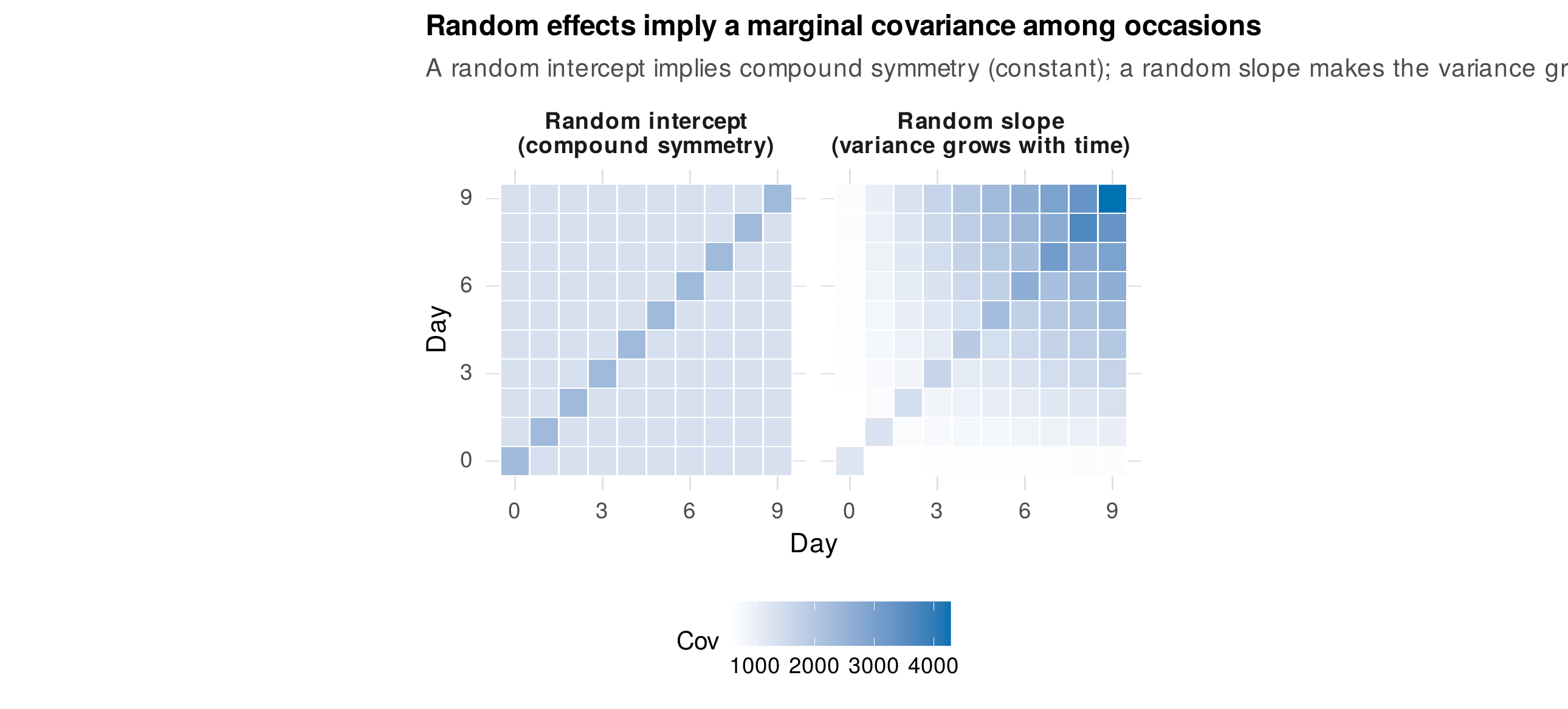
Note. The marginal covariance \(\mathbf{Z}_i\mathbf{T}\mathbf{Z}_i' + \sigma^2\mathbf{I}\) implied by two models. A random intercept (left) implies compound symmetry, a constant covariance between any two occasions, the structure the repeated-measures analysis of variance assumes. A random slope (right) implies a variance that grows with time and correlations that decay with separation, a structure no fixed covariance menu contains.
Table 13.1. One model, four literatures.
| Name | Field of origin | Emphasis |
|---|---|---|
| Hierarchical linear model | Education, sociology | Levels of nesting; contextual effects |
| Mixed-effects model | Statistics, biostatistics | Fixed plus random effects |
| Random-coefficients model | Econometrics | Coefficients varying across units |
| Variance-components model | Animal breeding, genetics | Partition of variance |
| Multilevel model | Cross-disciplinary | Data with a nested structure |
Note. These are names for the same model. The vocabulary differs because the model was developed independently in several fields, but the mathematics is identical, and results in one framework translate exactly into another.
13.2 Estimation: What the Software Does
The variance parameters are estimated by one of two likelihood methods, and the distinction matters in practice. Maximum likelihood (ML) estimates the variance components by maximizing the full likelihood, but it does so treating the fixed effects as known, which leaves the variance estimates biased downward in the same way that dividing a sample variance by \(n\) rather than \(n-1\) does. Restricted maximum likelihood (REML) removes this bias by estimating the variance components from residuals that have had the fixed effects projected out, and it is the appropriate default for reporting variance estimates. The two methods differ in one consequential way for model comparison: because REML changes the fixed-effects part of the likelihood, two models with different fixed effects cannot be compared by their REML likelihoods, so a likelihood-ratio test of fixed effects must be conducted under maximum likelihood, whereas a test of random effects may use either. Table 13.2 states the rules.
Table 13.2. Maximum likelihood versus restricted maximum likelihood.
| Task | Method | Reason |
|---|---|---|
| Reporting variance estimates | REML | Unbiased variance components |
| Comparing fixed-effect structures | ML | REML likelihoods not comparable across fixed effects |
| Comparing random-effect structures | Either (REML preferred) | Fixed part unchanged |
| Final reported model | REML | Best variance estimates |
Note. The practical protocol is to build and compare models with the appropriate method and to refit the final model under REML for reporting. Most software defaults to REML.
Estimation sometimes reaches a boundary, reported as a singular fit, in which a variance is estimated at zero or a random-effect correlation at plus or minus one. This is not an error but a message: the data do not contain enough information to estimate the requested random-effect structure, most often because there are too few clusters or too few occasions per cluster to identify a slope variance, or because two random effects are nearly collinear. The correct response is not to ignore the warning but to simplify the random structure in a principled way, and the troubleshooting protocol for doing so is developed in Section 13.5. Two software implementations divide the labor in R: lme4 is fast, handles crossed random effects, and is the workhorse for the models of this book, while nlme is slower but can fit residual covariance structures and heteroscedasticity directly, capabilities used for the growth models of Chapter 14. The reader should learn to read the output of a fitted model line by line, and the worked example of Section 13.6 annotates one in full.
13.3 Inference
Inference in the mixed model is subtler than in ordinary regression, and honesty about the subtlety is part of using the model well. For the fixed effects, the difficulty is that the exact distribution of the test statistic is unknown, because the denominator degrees of freedom are not a simple count when the data are unbalanced and the errors correlated. This is why the lme4 package deliberately reports no p-values: not because mixed models are controversial, but because there is no single correct degrees-of-freedom value to report. The practical resolutions are the Satterthwaite and Kenward-Roger approximations, which estimate an effective degrees of freedom and, for Kenward-Roger, also adjust the standard error; both are available in R and both are far better calibrated at small samples than the naive large-sample normal approximation. Figure 13.4 shows why the correction matters: in a simulation, the confidence interval built on the naive normal approximation under-covers badly when the number of clusters is small, dipping below ninety-two percent at six clusters, while the Satterthwaite interval holds near its nominal ninety-five percent throughout. The lesson is that with few clusters a degrees-of-freedom correction is not optional, and the Kenward-Roger method is preferred at the smallest samples (Luke, 2017; McNeish, 2017).
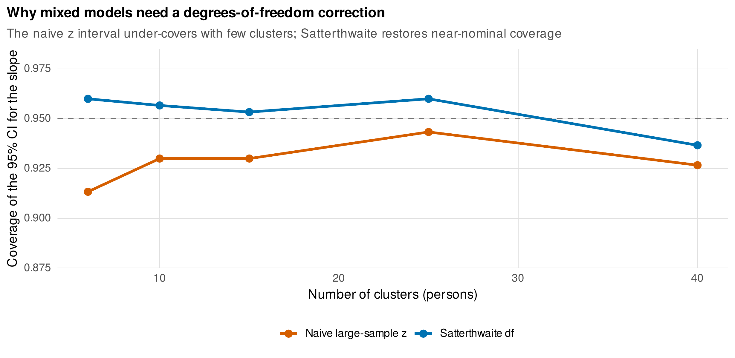
Note. Empirical coverage of the nominal ninety-five-percent confidence interval for a fixed slope, from a simulation, against the number of clusters. The naive large-sample interval under-covers with few clusters; the Satterthwaite degrees-of-freedom correction restores near-nominal coverage. Kenward-Roger performs similarly and is preferred at the smallest samples.
Inference on the variance components faces a different problem, that the null hypothesis places the parameter on the boundary of its space, because a variance cannot be negative. Testing whether a random slope is needed, that is whether its variance is zero, therefore cannot use the ordinary likelihood-ratio test with its usual chi-square reference, because the standard theory assumes the null value lies in the interior of the parameter space. Under the correct boundary theory, the likelihood-ratio statistic follows not a chi-square distribution but a mixture, with substantial probability mass at exactly zero (Self & Liang, 1987; Stram & Lee, 1994). Figure 13.5 shows the null distribution of the statistic from a simulation: a large spike at zero, because the unconstrained estimate of a variance is negative half the time and is then set to zero, together with a chi-square-shaped remainder that lies below the naive chi-square density. The naive test is therefore conservative, rejecting too rarely, and the correction is simply to halve the p-value, or equivalently to compare against the mixture. The practical implication reverses the usual worry: the danger is not false detection of a random slope but failure to detect one that is real.
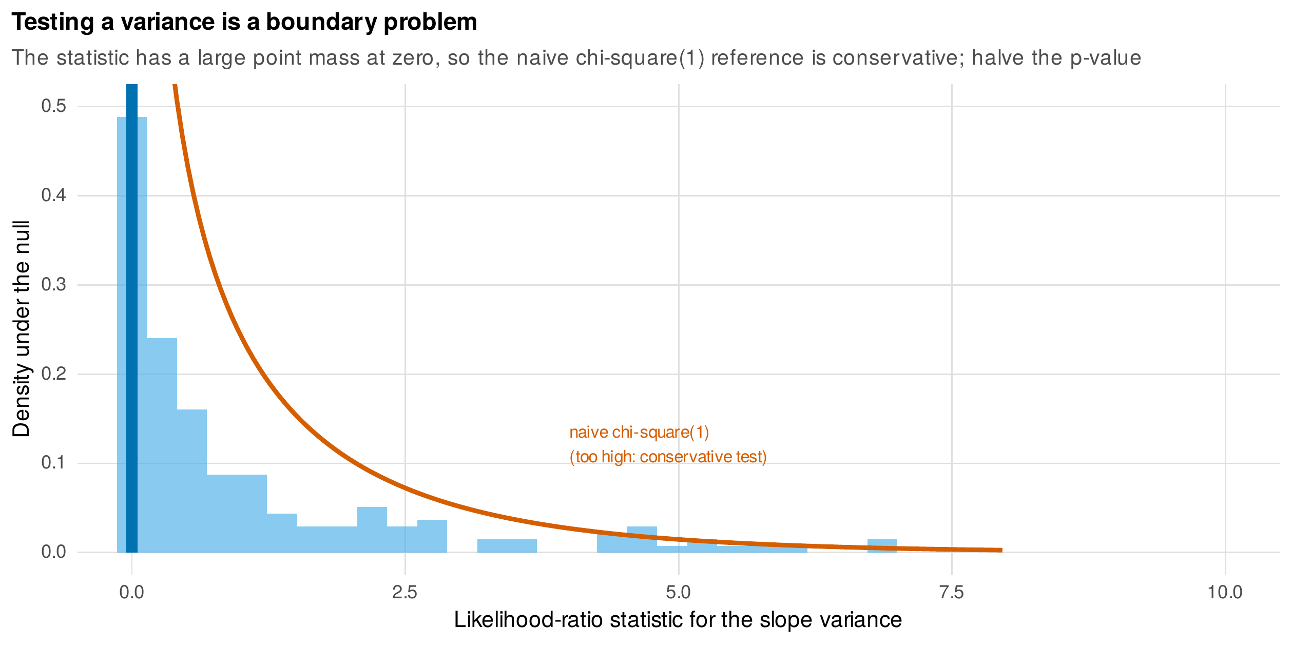
Note. The null distribution of the likelihood-ratio statistic for a slope variance, from a simulation, with a large point mass at zero and a positive part that lies below the naive chi-square density (red). Because the naive chi-square reference sits above the true null, the naive test is conservative; the correct test halves the p-value or uses the mixture reference.
The random effects also yield predictions of individual quantities, the best linear unbiased predictions (BLUPs), or conditional modes, which estimate each person’s own intercept and slope. These are not simply the person’s own ordinary-least-squares fit, but a shrinkage compromise between that fit and the population average, weighted by reliability, exactly the partial-pooling idea foreshadowed for person means in Chapter 7. A person with many reliable observations is trusted and their prediction stays near their own data; a person with few or noisy observations is shrunk toward the group, on the principle that when an individual estimate is unreliable the group is a better guess. Figure 13.6 shows the effect on the sleepstudy subjects: the per-person ordinary-least-squares estimates are pulled inward toward the pooled estimate, the more so the less reliable they are. The Foundations box gives the shrinkage weight explicitly. These predictions are valuable for description, for caterpillar plots and individual-trajectory displays, but they must be used cautiously as inputs to a second analysis, because treating shrunken estimates as if they were observed data understates their uncertainty and biases downstream results. Table 13.3 collects the inference options.
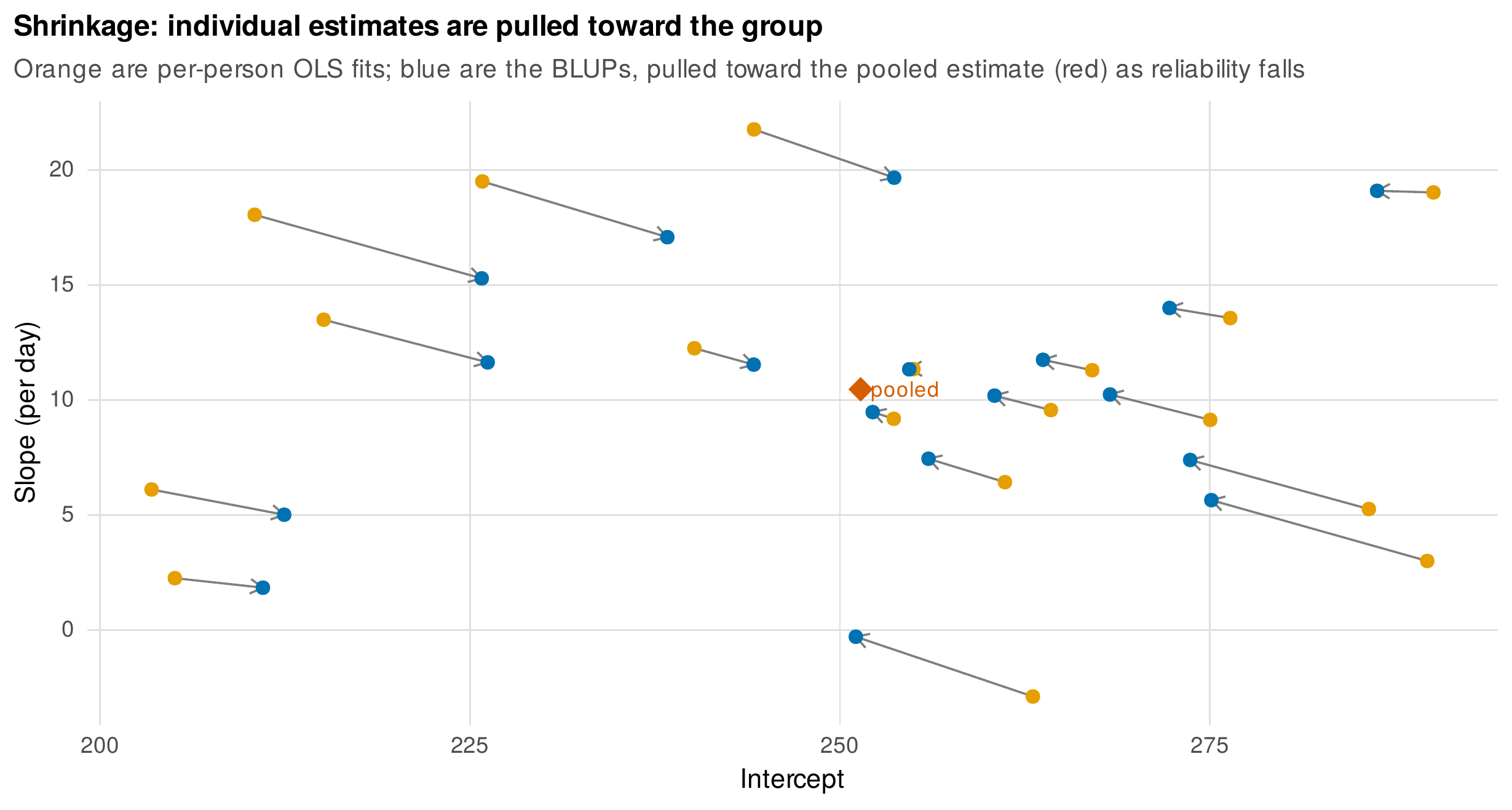
Note. Per-person ordinary-least-squares estimates of the intercept and slope (orange) and the model’s best linear unbiased predictions (blue) for the sleepstudy subjects, with arrows from one to the other. The predictions are pulled toward the pooled estimate (red), the more so the less reliable a person’s own estimate, which is the partial-pooling compromise the Foundations box derives.
Foundations Box • Shrinkage as a reliability-weighted compromise
For a person’s random intercept, the best linear unbiased prediction is \(\hat{u}_{0i} = \lambda_i (\bar{y}_i - \hat{\gamma}_{00})\), where \(\bar{y}_i - \hat{\gamma}_{00}\) is the person’s raw deviation from the grand mean and \(\lambda_i = \tau_{00} / (\tau_{00} + \sigma^2/n_i)\) is a reliability that ranges from zero to one. When a person has many observations, \(\sigma^2/n_i\) is small, \(\lambda_i\) approaches one, and the prediction is nearly the person’s own deviation. When a person has few observations, \(\sigma^2/n_i\) is large, \(\lambda_i\) approaches zero, and the prediction is shrunk toward the group mean of zero. The reliability \(\lambda_i\) is exactly the intraclass-correlation logic of Chapter 7 applied to one person’s mean, which is why the person means of that chapter were flagged as noisy: the mixed model replaces them with shrinkage estimates that borrow strength from the group in proportion to each person’s unreliability. The same logic applied to a variance test gives the mixture reference of Figure 13.5, because the constrained estimate of a variance is the unconstrained estimate shrunk up to the zero boundary.
Table 13.3. Inference options in the mixed model.
| Target | Method | Note |
|---|---|---|
| Fixed effect | Satterthwaite or Kenward-Roger df | Corrects small-sample under-coverage; KR preferred at smallest \(N\) |
| Fixed effect | Likelihood-ratio test (under ML) | Compare nested fixed structures |
| Fixed effect | Parametric bootstrap; profile CI | Most reliable but computationally heavy |
| Variance component | Boundary-corrected LRT | Halve the p-value; mixture reference |
| Individual effect | BLUP with conditional variance | Description, not uncritical two-stage input |
Note. The single most common error is to report a fixed-effect test with uncorrected degrees of freedom or a variance test with an uncorrected chi-square. Both corrections are available and should be used.
Whether a slope should be modeled as random is partly a statistical question and partly a design question, and it has been the subject of a genuine debate. One position holds that a confirmatory analysis should include the maximal random-effects structure justified by the design, so that a random slope is included for every within-cluster predictor whose effect is tested, on the grounds that omitting it inflates the false-positive rate (Barr et al., 2013). The opposing position holds that a maximal structure is often unsupportable by the data, producing the singular fits of Section 13.2 and a loss of power, and that the random structure should be pared to what the data can identify (Matuschek et al., 2017). The debate originates in experimental psycholinguistics, where designs are balanced and clusters plentiful, and it must be translated with care to the longitudinal setting, where occasions per person are often few. The book’s position is a middle one: include random slopes for the within-person effects central to the theory, simplify when the data cannot support the full structure rather than forcing a singular fit, and report the sensitivity of the fixed-effect conclusions to the random structure chosen. The In Practice box digests the debate.
In Practice • the keep-it-maximal debate, resolved for practice
The maximal position (Barr et al., 2013) and the parsimonious position (Matuschek et al., 2017) are both right about something. Omitting a random slope that genuinely varies does inflate the false-positive rate of the corresponding fixed effect, because the model then treats correlated observations as independent evidence. But forcing a maximal structure the data cannot identify produces a singular fit, wastes power, and can make the intended fixed-effect test unstable. The workable resolution has three parts. First, let theory choose the candidate random slopes: a within-person predictor whose effect is the research question earns a random slope. Second, let the data arbitrate feasibility: if the maximal model is singular, drop the random-effect correlations first (the (x || id) specification), then the least theoretically central slope, until the fit is non-singular. Third, report the sensitivity: state the random structure, note whether the fixed-effect conclusion survives a simpler and a richer structure, and let the reader see that the result does not hinge on an arbitrary choice.
13.4 Centering: The Decision That Changes the Question
The most consequential and most often mishandled decision in a longitudinal mixed model is how to center a time-varying predictor, because the centering determines which of two different questions the predictor’s coefficient answers. This is the full treatment promised since Chapter 1. A time-varying predictor \(x_{it}\) decomposes, as in Chapter 7, into a person mean \(\bar{x}_{i\cdot}\) and a within-person deviation \(x_{it} - \bar{x}_{i\cdot}\), and the two components can relate to the outcome in entirely different ways. Person-mean centering, also called centering within cluster, enters the deviation \(x_{it} - \bar{x}_{i\cdot}\) so that its coefficient is the pure within-person effect, the expected change in the outcome when a person is one unit above their own usual level. Adding the person mean \(\bar{x}_{i\cdot}\) as a second, level-two predictor lets its coefficient capture the between-person effect, the expected difference in the outcome between two people who differ by one unit in their usual level. By contrast, entering the raw predictor \(x_{it}\) without the person mean forces a single coefficient to serve both roles, and that coefficient is a variance-weighted blend of the within and between effects, equal to neither unless the two happen to coincide. Grand-mean centering shifts the intercept but leaves this conflation intact, because it changes the origin without separating the levels.
The stakes are highest when the within and between effects have opposite signs, and Figure 13.7 shows exactly this in the caffeine-and-tiredness data introduced in Chapter 1. Within persons, drinking more caffeine than usual is associated with feeling less tired, a negative within-person effect of \(-0.78\); between persons, people who habitually drink more caffeine are more tired, a positive between-person effect of \(+0.89\), presumably because tiredness drives habitual consumption. The raw coefficient of \(-0.78\) captures only the within story and entirely conceals the positive between-person association, an instance of the ecological fallacy that person-mean centering exists to prevent. The figure also shows a same-signed case, the stress-and-negative-affect data, where the within effect (\(0.35\)) and the between effect (\(0.46\)) point the same way but still differ in magnitude, so that the raw coefficient conflates two distinct quantities even when it does not mislead about sign. The contextual effect, the difference between the between and within coefficients, is often the substantive quantity of interest, measuring how much a person’s standing relative to others matters over and above their momentary state (Enders & Tofighi, 2007; Curran & Bauer, 2011). An equivalent parameterization, the Mundlak specification, enters the raw predictor together with the person mean and reads the person-mean coefficient directly as the contextual effect; it recovers the same within effect and connects the mixed model to the fixed-effects estimator of econometrics, a bridge revisited in the cross-lagged models of Chapter 21. Table 13.4 is the master centering table.
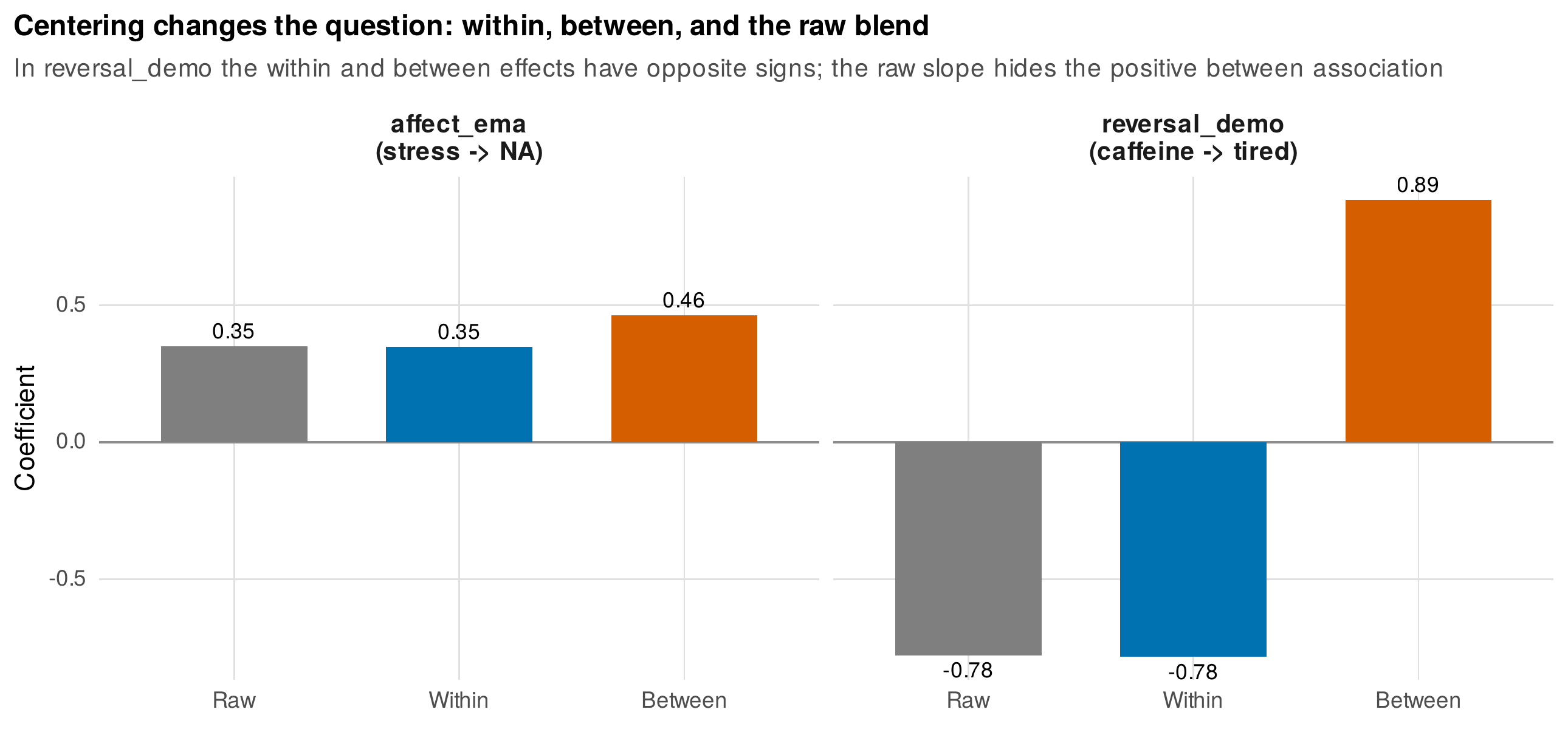
Note. Coefficients from raw, within-person (person-mean-centered), and between-person (person-mean) specifications. Left: for stress and negative affect the effects are same-signed but different in magnitude. Right: for caffeine and tiredness the within effect is negative and the between effect positive, and the raw coefficient hides the positive between-person association entirely. Only person-mean centering separates the two.
Table 13.4. Centering choices and the estimand.
| Specification | Predictors entered | The slope estimates |
|---|---|---|
| Raw | \(x_{it}\) | A blend of within and between; neither, in general |
| Grand-mean centered | \(x_{it} - \bar{x}\) | The same blend, with a shifted intercept |
| Person-mean centered | \(x_{it} - \bar{x}_{i\cdot}\) | The pure within-person effect |
| Centered plus mean | \((x_{it} - \bar{x}_{i\cdot})\) and \(\bar{x}_{i\cdot}\) | Within (deviation) and between (mean) separately |
| Mundlak | \(x_{it}\) and \(\bar{x}_{i\cdot}\) | Within (raw) and contextual (mean) |
Note. The choice is not cosmetic: it determines whether the coefficient answers a within-person or a between-person question. For within-person research questions, person-mean centering is required, and the person mean should be entered so the between effect is not discarded.
13.5 The Practical Workflow
Building a mixed model is a sequence of principled decisions, not a single command, and documenting the sequence is part of the analysis. A sound strategy begins with an unconditional means model, a random intercept and no predictors, which yields the intraclass correlation and confirms that a multilevel structure is warranted; adds the fixed effect of time and any theory-driven fixed predictors; adds random slopes for the within-person effects of central interest; and compares the successive models by the appropriate likelihood method, maximum likelihood for fixed-effect changes and either for random-effect changes. Every step is recorded in a model-building table, the template of Table 13.5, so that a reader can follow the reasoning from null model to final specification. When estimation fails to converge or returns a singular fit, the troubleshooting protocol of Figure 13.8 applies in order: rescale and center the predictors so the optimizer works on comparable scales, simplify the random structure by first removing correlations and then the least central slope, switch or combine optimizers, increase the iteration limit, and, as a last resort for a structure the data genuinely cannot support by likelihood, move to the Bayesian estimation of Chapter 17, whose priors can regularize a weakly identified variance.
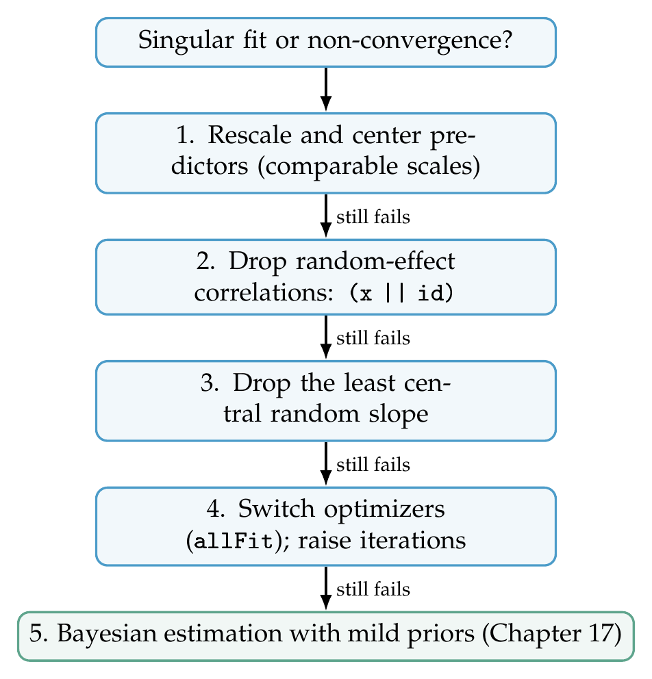
Note. Applied in order when a mixed model fails to converge or returns a singular fit. Each step addresses a common cause, from ill-scaled predictors through an over-ambitious random structure to optimizer settings; the last resort is Bayesian estimation, whose priors regularize a variance the likelihood cannot identify. A singular fit is a message about the data, not an error to suppress.
A fitted model must be diagnosed, and the mixed model has residuals and assumptions at two levels. Figure 13.9 shows the panel for the sleepstudy model: the level-one residuals should be homoscedastic and roughly normal, checked against the fitted values and in a quantile plot; the random effects should be approximately normal, checked in their own quantile plot; and the joint distribution of the random intercept and slope reveals their correlation and any outlying persons. Reassuringly, the fixed-effect estimates of a mixed model are fairly robust to non-normality of the random effects, so a mild departure in the random-effect quantile plot is not fatal, though a person with extreme influence deserves scrutiny (Schielzeth et al., 2020). Finally, the variance explained is summarized by the marginal and conditional R-squared of Nakagawa and Schielzeth (2013): the marginal, here \(0.30\), is the proportion of variance explained by the fixed effects alone, and the conditional, here \(0.79\), is the proportion explained by the fixed and random effects together, the gap between them measuring how much the individual differences add. The more complete Rights and Sterba (2019) framework decomposes the explained variance into interpretable within- and between-cluster sources and is the serious answer where the sources matter, with the Nakagawa measures serving as the common currency; both should be reported in preference to a naive pseudo-R-squared, which can behave paradoxically and even decrease when a useful predictor is added.
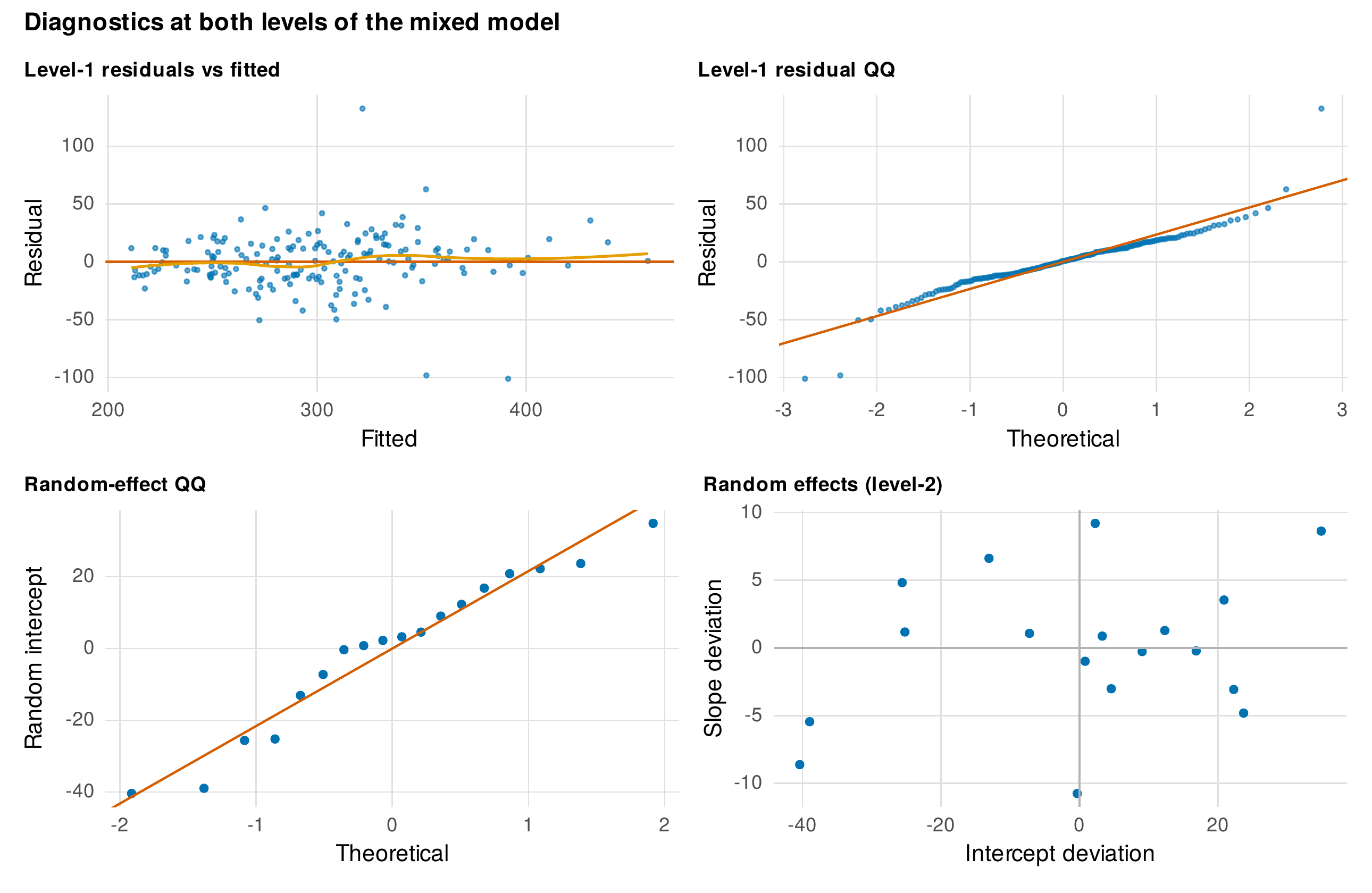
Note. For the sleepstudy model: level-one residuals against fitted values and in a quantile plot (top), the random-intercept quantile plot and the joint distribution of the random intercept and slope (bottom). The mixed model has assumptions at both levels; its fixed effects are fairly robust to mild non-normality of the random effects, but influential persons warrant scrutiny.
Table 13.5. A model-building documentation template.
| Model | Specification | Estimation | Purpose |
|---|---|---|---|
| M0 | Intercept, random intercept | REML | Intraclass correlation; is nesting present |
| M1 | \(+\) fixed time | ML | Average trajectory |
| M2 | \(+\) fixed covariates | ML | Theory-driven effects |
| M3 | \(+\) random slope of time | REML | Individual differences in change |
| M4 | \(+\) cross-level interaction | ML | Moderation of change |
| Final | Selected model | REML | Reported estimates |
Note. Documenting the sequence lets a reader follow the reasoning from null model to final specification and see which effects survived which comparison. Fixed-effect comparisons use maximum likelihood; the reported model is refitted under restricted maximum likelihood.
13.6 Worked Example and Reporting
The sleepstudy data carry the full arc. The unconditional model gives an intraclass correlation of \(0.39\), so more than a third of the variance in reaction time is stable between persons and a multilevel model is warranted. Adding the fixed effect of days establishes the average trajectory, an increase of about ten milliseconds per day of sleep deprivation. Adding a random slope reveals that people differ substantially in this rate, with a slope standard deviation of about six milliseconds per day, and the intercept-slope correlation is near zero, so initial reaction time does not predict the rate of deterioration. The final fitted model is shown over the data and as a caterpillar of individual slopes in Figure 13.10, the two model-over-data displays that Chapter 8 established as standard. The fixed effect of days is estimated at \(10.47\) milliseconds per day with a Satterthwaite-corrected test (\(SE = 1.55\), \(t = 6.77\), \(\mathit{df} = 17\), \(p < .001\)), and the marginal and conditional R-squared are \(0.30\) and \(0.79\). A model paragraph reads: “Reaction time was modeled with a linear mixed model including a fixed effect of days, a random intercept, and a random slope of days across subjects, estimated by restricted maximum likelihood in lme4 with Satterthwaite degrees of freedom from lmerTest. Reaction time increased by \(10.47\) ms per day (\(SE = 1.55\), \(\mathit{df} = 17\), \(p < .001\)). Subjects varied substantially in their rate of increase (slope \(SD = 5.9\) ms/day), and the intercept-slope correlation was negligible. The fixed and random effects together accounted for \(79\%\) of the variance (marginal \(R^2 = .30\)).” Table 13.6 is the reporting checklist this paragraph satisfies, and it is the standard reused by the growth, generalized, and intensive-data chapters that follow.
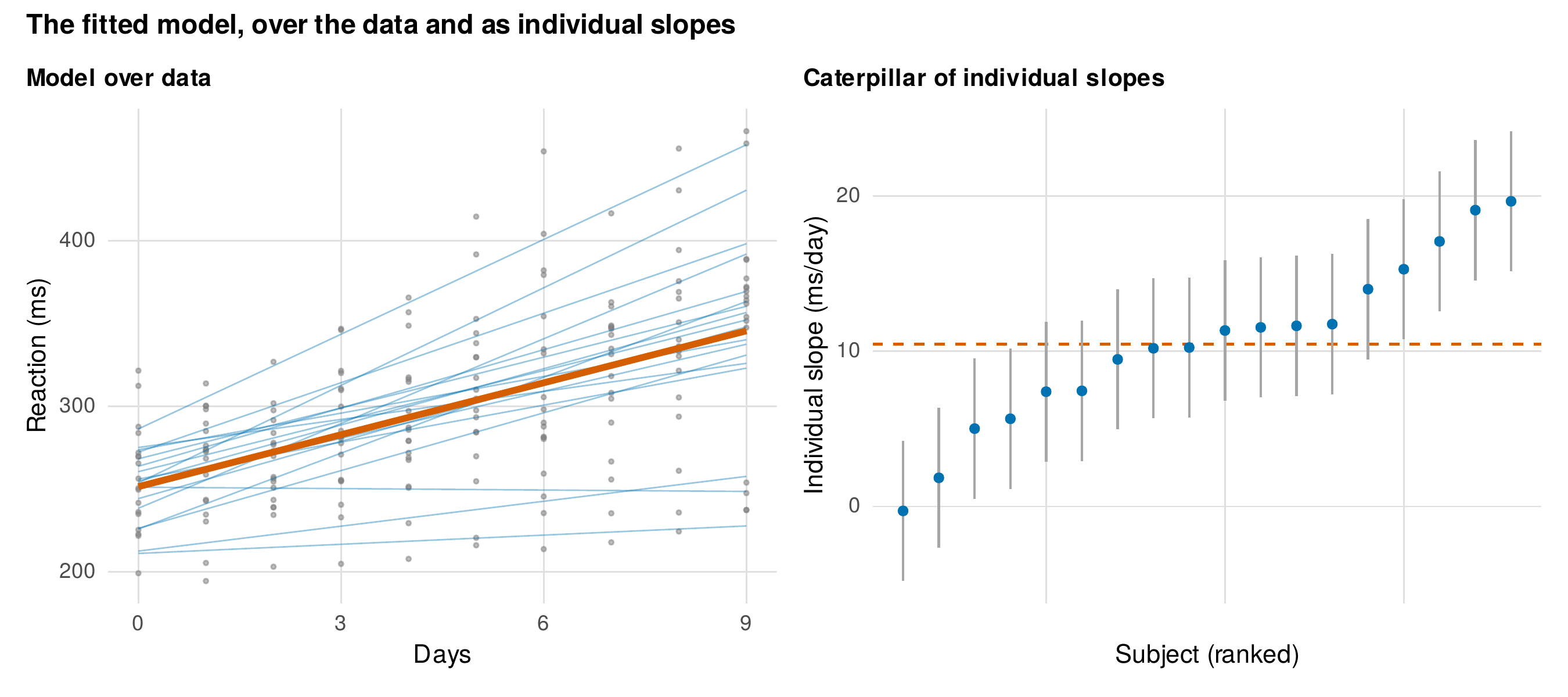
Note. Left: the fitted sleepstudy model, with individual predicted trajectories (blue) and the fixed-effect trajectory (red) over the observed data. Right: a caterpillar plot of the individual slopes with their intervals, ranked; subjects whose interval excludes the average slope (dashed) deteriorate reliably faster or slower than typical. These are the two standard model-over-data displays of Chapter 8.
Table 13.6. Reporting checklist for linear mixed models.
| Element | What to report |
|---|---|
| Model specification | Fixed effects, random effects, and the level each varies at, in hierarchical or combined form |
| Estimation | Method (ML/REML), software and version, optimizer if nonstandard |
| Fixed-effect inference | Estimates, standard errors, and the degrees-of-freedom method (Satterthwaite/Kenward-Roger) |
| Random effects | Variances, the intercept-slope correlation, and the residual variance, with the test method for any |
| Centering | How time-varying predictors were centered and what each coefficient estimates |
| Model building | The sequence of models compared and the criterion for the final choice |
| Variance explained | Marginal and conditional \(R^2\); convergence and singular-fit notes |
Note. The checklist is the book standard, reused in Chapters 14 through 16 and 23. Its omissions in practice are usually the degrees-of-freedom method, the centering choice, and the random-structure justification, each of which changes what the reported numbers mean.
13.7 Running the Mixed Model in R
The model is fitted with lmer from lme4, and the Satterthwaite tests come from loading lmerTest, which adds degrees of freedom and p-values to the summary. The model-building sequence and the centering are a few lines each.
library(lme4); library(lmerTest); library(dplyr)
data(sleepstudy)

m0 <- lmer(Reaction ~ 1 + (1 | Subject), sleepstudy)             # null: ICC
m1 <- lmer(Reaction ~ Days + (1 | Subject), sleepstudy)          # + fixed slope
m2 <- lmer(Reaction ~ Days + (Days | Subject), sleepstudy)       # + random slope
summary(m2)                                                       # Satterthwaite df via lmerTest
ranova(m2)                                                        # boundary-corrected test of the random slope
VarCorr(m2); confint(m2)                                          # variances; profile CIs
The person-mean centering that separates the within and between effects is a grouped transformation followed by entering both components, and the marginal and conditional R-squared come from the variance of the predictions.
# --- Within/between decomposition by person-mean centering ---
ae <- readRDS("Examples/data/affect_ema.rds") |>
  filter(!is.na(na), !is.na(stress)) |>
  group_by(person) |> mutate(pm = mean(stress), cwc = stress - pm) |> ungroup()
lmer(na ~ cwc + pm + (1 | person), ae)     # cwc = within effect; pm = between effect

# --- Nakagawa marginal / conditional R^2 ---
vf <- var(predict(m2, re.form = NA)); vt <- var(predict(m2)); ve <- sigma(m2)^2
c(marginal = vf/(vf + (vt-vf) + ve), conditional = (vt)/(vt + ve))
The complete analysis, including the boundary-LRT and Satterthwaite-coverage simulations and the shrinkage computation, is the shipped script ch13_analysis_V01.R, with figures drawn by ch13_figures_V01.R. The nlme package fits the same models with a different syntax and adds residual covariance structures used in Chapter 14, and the performance and r2mlm packages compute the variance-explained measures automatically.
Software Note • reading the same model across software
The linear mixed model is fitted by MIXED in SPSS, mixed in Stata, PROC MIXED in SAS, and the HLM program, and their outputs map onto one another once the vocabulary of Table 13.1 is known: what lme4 prints as random-effect variances SPSS labels covariance parameters and HLM labels tau. Two cross-software cautions matter. First, the default degrees-of-freedom method differs, SAS and Stata offering Kenward-Roger or Satterthwaite while some defaults are the naive large-sample value, so the method must be set deliberately and reported. Second, the default estimation is REML in most packages but the comparison of fixed effects requires ML, a switch each program exposes differently. The Mplus TYPE = TWOLEVEL framework fits the same model in the structural-equation parameterization that Chapter 19 develops, where the equivalence of the mixed and latent-growth models becomes explicit.
13.8 Common Misconceptions
Several beliefs about mixed models mislead. The first is that random effects are nuisance corrections for non-independence; often they are the phenomenon itself, the individual differences in change that motivate the study, and the slope variance and intercept-slope correlation are substantive findings, not statistical bookkeeping. The second is that lme4’s refusal to print p-values means mixed models are controversial; it reflects only the genuine difficulty of the denominator degrees of freedom, resolved by the Satterthwaite and Kenward-Roger corrections. The third is a pair of opposite errors about the random structure, that more random effects is always safer and that a singular fit means the model is wrong; the truth is that the random structure should match what theory requires and the data can support, and a singular fit is a message to simplify, not a verdict of failure. The fourth is that the intraclass correlation from the null model stays meaningful after predictors are added; once predictors enter, the variance components are conditional, and the null-model intraclass correlation no longer describes the fitted model. A recurring question, how many clusters and occasions are needed, has the honest answer that it depends on the effect and the design, is best settled by the simulation-based power analysis of Chapter 4, and that fixed effects tolerate fewer clusters than variance components, which are poorly estimated below roughly thirty clusters.
Common Pitfall • four errors in mixed-model practice
First, comparing REML deviances across fixed structures: REML likelihoods are not comparable when the fixed effects differ, so a likelihood-ratio test of a fixed effect must be refitted under maximum likelihood. Second, treating a singular fit as a reason to strip all random slopes: the fix is to simplify in order, dropping correlations first, not to abandon the random structure the theory requires. Third, interpreting a raw-score coefficient as a within-person effect: without person-mean centering, the coefficient is a blend of within and between effects and can even carry the wrong sign (Figure 13.7). Fourth, reading a decreasing pseudo-R-squared as worse fit: some pseudo-R-squared measures can fall when a useful predictor is added, an artifact of their construction; use the marginal and conditional measures, or the Rights-Sterba decomposition.
Chapter Summary
The linear mixed model is the book’s central tool. It is written in a hierarchical form, with person-specific lines whose coefficients vary around population averages, and an equivalent combined form separating fixed effects, random effects, and residual (Figure 13.1); the random-effect covariance, the T matrix, describes individual differences in level and in change and their correlation, the shape of which is the fan-spread or fan-close of the trajectories (Figure 13.2). The random effects imply a marginal covariance \(\mathbf{Z}_i\mathbf{T}\mathbf{Z}_i' + \sigma^2\mathbf{I}\) that subsumes the sphericity of the analysis of variance and the working correlation of the marginal model (Figure 13.3). Estimation is by maximum likelihood or, for unbiased variances, restricted maximum likelihood, and a singular fit is a message that the data cannot support the requested random structure. Inference on fixed effects needs a Satterthwaite or Kenward-Roger degrees-of-freedom correction, which restores coverage at small samples (Figure 13.4); inference on a variance is a boundary problem whose naive chi-square test is conservative (Figure 13.5); and individual effects are shrinkage predictions that borrow strength from the group in proportion to unreliability (Figure 13.6). Person-mean centering separates the within-person from the between-person effect of a time-varying predictor, effects that can differ in magnitude or even in sign, so that the raw coefficient answers neither question cleanly (Figure 13.7). The model is built by a documented sequence, troubleshot by an ordered protocol (Figure 13.8), diagnosed at both levels (Figure 13.9), summarized by marginal and conditional variance explained, and reported to a standard checklist (Figure 13.10).
Where to Go Next
Everything in Parts IV through VI builds on this chapter. Chapter 14 specializes the model to growth, where time is the central predictor and the trajectory’s shape, linear, polynomial, or piecewise, becomes the object of study. Chapters 15 and 16 extend it to non-normal outcomes through the generalized linear mixed model, the subject-specific counterpart to Chapter 12’s marginal model, and to modeling the within-person variance itself. Chapter 17 supplies the Bayesian estimation that rescues the weakly identified random structures this chapter’s troubleshooting protocol ends with. Chapter 19 reveals the latent-growth model to be the same model in structural-equation form, making the implied covariance of Section 13.1 explicit as a factor structure. Chapter 21 develops the fixed-effects and centering bridge into the cross-lagged panel debates, and Chapter 23 deploys the whole apparatus on intensive longitudinal data. The notation and the workflow established here are the common language of all of them, and the centering section in particular is the book’s most-cited, because the within-and-between distinction recurs wherever a time-varying predictor appears.
Exercises
- 13.1 Translate the forms. For a given two-level model, write the hierarchical and combined forms, and interpret every fixed effect, variance, covariance, and residual in words.
- 13.2 Build a sequence. On a provided longitudinal dataset, build the model sequence from null to final, document each step in a model-building table, and defend the final random structure against a simpler and a richer alternative.
- 13.3 Center three ways. Fit raw, grand-mean-centered, and person-mean-centered specifications of a time-varying predictor, and write the three interpretations, identifying which coefficient answers the within-person question.
- 13.4 Coverage simulation. By simulation, estimate the coverage of the Satterthwaite confidence interval for a fixed slope at fifteen clusters, and compare it to the naive interval.
- 13.5 Diagnose and repair. Given a non-converging model with planted problems (an unscaled time variable and an overparameterized random structure), apply the troubleshooting protocol and report the working model.
- 13.6 Boundary test. By simulation, verify that the likelihood-ratio statistic for a slope variance has a point mass at zero under the null, and show that the naive chi-square test is conservative.
References
Barr, D. J., Levy, R., Scheepers, C., & Tily, H. J. (2013). Random effects structure for confirmatory hypothesis testing: Keep it maximal. Journal of Memory and Language, 68(3), 255–278. https://doi.org/10.1016/j.jml.2012.11.001
Bates, D., Mächler, M., Bolker, B., & Walker, S. (2015). Fitting linear mixed-effects models using lme4. Journal of Statistical Software, 67(1), 1–48. https://doi.org/10.18637/jss.v067.i01
Curran, P. J., & Bauer, D. J. (2011). The disaggregation of within-person and between-person effects in longitudinal models of change. Annual Review of Psychology, 62, 583–619. https://doi.org/10.1146/annurev.psych.093008.100356
Enders, C. K., & Tofighi, D. (2007). Centering predictor variables in cross-sectional multilevel models: A new look at an old issue. Psychological Methods, 12(2), 121–138. https://doi.org/10.1037/1082-989X.12.2.121
Hamaker, E. L., & Grasman, R. P. P. P. (2015). To center or not to center? Investigating inertia with a multilevel autoregressive model. Frontiers in Psychology, 5, Article 1492. https://doi.org/10.3389/fpsyg.2014.01492
Hox, J. J., Moerbeek, M., & van de Schoot, R. (2018). Multilevel analysis: Techniques and applications (3rd ed.). Routledge. https://doi.org/10.4324/9781315650982
Kenward, M. G., & Roger, J. H. (1997). Small sample inference for fixed effects from restricted maximum likelihood. Biometrics, 53(3), 983–997. https://doi.org/10.2307/2533558
Kuznetsova, A., Brockhoff, P. B., & Christensen, R. H. B. (2017). lmerTest package: Tests in linear mixed effects models. Journal of Statistical Software, 82(13), 1–26. https://doi.org/10.18637/jss.v082.i13
Laird, N. M., & Ware, J. H. (1982). Random-effects models for longitudinal data. Biometrics, 38(4), 963–974. https://doi.org/10.2307/2529876
Luke, S. G. (2017). Evaluating significance in linear mixed-effects models in R. Behavior Research Methods, 49(4), 1494–1502. https://doi.org/10.3758/s13428-016-0809-y
Matuschek, H., Kliegl, R., Vasishth, S., Baayen, H., & Bates, D. (2017). Balancing Type I error and power in linear mixed models. Journal of Memory and Language, 94, 305–315. https://doi.org/10.1016/j.jml.2017.01.001
McNeish, D. (2017). Small sample methods for multilevel modeling: A colloquial elucidation of REML and the Kenward-Roger correction. Multivariate Behavioral Research, 52(5), 661–670. https://doi.org/10.1080/00273171.2017.1344538
Nakagawa, S., & Schielzeth, H. (2013). A general and simple method for obtaining \(R^2\) from generalized linear mixed-effects models. Methods in Ecology and Evolution, 4(2), 133–142. https://doi.org/10.1111/j.2041-210x.2012.00261.x
Pinheiro, J. C., & Bates, D. M. (2000). Mixed-effects models in S and S-PLUS. Springer. https://doi.org/10.1007/b98882
Raudenbush, S. W., & Bryk, A. S. (2002). Hierarchical linear models: Applications and data analysis methods (2nd ed.). Sage.
Rights, J. D., & Sterba, S. K. (2019). Quantifying explained variance in multilevel models: An integrative framework for defining R-squared measures. Psychological Methods, 24(3), 309–338. https://doi.org/10.1037/met0000184
Schielzeth, H., Dingemanse, N. J., Nakagawa, S., Westneat, D. F., Allegue, H., Teplitsky, C., Réale, D., Dochtermann, N. A., Garamszegi, L. Z., & Araya-Ajoy, Y. G. (2020). Robustness of linear mixed-effects models to violations of distributional assumptions. Methods in Ecology and Evolution, 11(9), 1141–1152. https://doi.org/10.1111/2041-210X.13434
Self, S. G., & Liang, K.-Y. (1987). Asymptotic properties of maximum likelihood estimators and likelihood ratio tests under nonstandard conditions. Journal of the American Statistical Association, 82(398), 605–610. https://doi.org/10.1080/01621459.1987.10478472
Snijders, T. A. B., & Bosker, R. J. (2012). Multilevel analysis: An introduction to basic and advanced multilevel modeling (2nd ed.). Sage.
Stram, D. O., & Lee, J. W. (1994). Variance components testing in the longitudinal mixed effects model. Biometrics, 50(4), 1171–1177. https://doi.org/10.2307/2533455
Verbeke, G., & Molenberghs, G. (2000). Linear mixed models for longitudinal data. Springer. https://doi.org/10.1007/978-1-4419-0300-6