Chapter 14
Growth Curve Modeling in the Multilevel Framework
The mixed model of the previous chapter treated time as one predictor among others. This chapter makes time the protagonist. When the predictor whose slope varies across people is time itself, the person-specific line becomes a person-specific trajectory, its intercept becomes a starting level, and its slope becomes a rate of change, and the random-effect covariance that seemed abstract in Chapter 13 becomes the substance of the science: how much people differ in where they begin, how much they differ in how fast they change, and whether those two differences are linked. The growth curve model is nothing more than the linear mixed model with time as the level-one predictor, and everything established in Chapter 13, the estimation by likelihood, the boundary problems of variance testing, the centering logic, carries over without change. What is new is a set of decisions that only arise when time is the predictor: where to put the origin of the time axis, what functional shape the trajectory should take, how to accommodate people who are measured at different ages or on different schedules, how a person-level covariate reshapes the whole trajectory, and how to model residual dependence that the random effects leave behind. Each of these is a modeling choice with a substantive consequence, and each is developed here with the equation, the plain-language interpretation, and a worked demonstration on real trajectories.
Learning Objectives
After working through this chapter, you should be able to: (1) write the unconditional linear growth model as a mixed model and interpret its fixed effects, random-effect variances, and intercept-slope covariance as features of individual trajectories; (2) choose and justify the origin of the time metric, and explain how recoding time changes the intercept, its variance, and its correlation with the slope while leaving the slope itself unchanged; (3) specify nonlinear change through polynomial, piecewise-linear, and spline bases, and compare their fit; (4) fit a single growth model across cohorts measured on overlapping age ranges through the accelerated longitudinal design, and state its linkage assumption; (5) add person-level covariates as predictors of the intercept and slope, reading the resulting cross-level interactions as moderated change; (6) include a time-varying covariate in a growth model and separate its within-person from its between-person effect; (7) model residual covariance structure with nlme when the random effects do not fully capture dependence; and (8) build, diagnose, and report a growth model to publication standard.
14.1 Growth as a Mixed Model: Time as the Predictor
The unconditional linear growth model is the two-level mixed model of Chapter 13 with time inserted as the sole level-one predictor. At level one, each person’s outcome on each occasion is a person-specific line in time plus residual, \(y_{it} = \pi_{0i} + \pi_{1i}\,a_{it} + e_{it}\), where \(a_{it}\) is the value of the time metric for person \(i\) on occasion \(t\), \(\pi_{0i}\) is person \(i\)’s intercept, the expected outcome when \(a_{it}=0\), and \(\pi_{1i}\) is person \(i\)’s slope, the expected change in outcome per unit of time. The Greek letter \(\pi\) for the person-specific coefficients follows the growth-modeling convention of Raudenbush and Bryk (2002) and of Singer and Willett (2003), and it is the same object that Chapter 13 wrote as \(\beta_i\). At level two, each person’s intercept and slope are a population average plus a personal departure, \(\pi_{0i} = \gamma_{00} + u_{0i}\) and \(\pi_{1i} = \gamma_{10} + u_{1i}\), with the departures distributed bivariate normal, \((u_{0i}, u_{1i})' \sim N(\mathbf{0}, \mathbf{T})\), where the covariance matrix \(\mathbf{T}\) has the intercept variance \(\tau_{00}\), the slope variance \(\tau_{11}\), and their covariance \(\tau_{01}\) on and off its diagonal. The combined form, \(y_{it} = \gamma_{00} + \gamma_{10}a_{it} + u_{0i} + u_{1i}a_{it} + e_{it}\), is exactly the random-slope model of Chapter 13, and reading it as growth requires only the recognition that the varying predictor is time.
The three variance parameters are the empirical content of a growth study. The intercept variance \(\tau_{00}\) measures how widely people differ at the moment defined as time zero; the slope variance \(\tau_{11}\) measures how widely they differ in rate of change, and a slope variance indistinguishable from zero is the finding that everyone changes at essentially the same rate, however large the average change; and the intercept-slope covariance \(\tau_{01}\), usually reported as a correlation, states whether people who start higher change faster or more slowly than people who start lower. This last quantity answers whether individual differences in the outcome widen or narrow over time, the fan-spread or fan-close of Chapter 13, and in developmental and educational applications it is frequently the primary question, because it distinguishes a process in which early advantages compound from one in which laggards catch up. A growth model that reports only the average trajectory, the fixed effects \(\gamma_{00}\) and \(\gamma_{10}\), has discarded the individual differences that motivated measuring change in the first place.
The running dataset for this chapter is school_growth, a simulated cohort of 1,200 children, each measured on four occasions and nested within schools, whose academic achievement is recorded across grades three through eight. Fitting the unconditional linear model with the time metric centered at grade three, so that \(a_{it} = \text{grade} - 3\), gives an average starting level of \(\gamma_{00} = 188.1\) points at grade three and an average gain of \(\gamma_{10} = 8.39\) points per grade. The estimated child-level standard deviations are \(20.1\) points for the intercept and \(3.09\) points per grade for the slope, with an intercept-slope correlation of \(-0.25\), and the school level contributes a further intercept standard deviation of \(8.7\) points, with a residual standard deviation of \(9.1\). The negative intercept-slope correlation says that, at this origin, children who begin third grade higher tend to gain slightly more slowly, a mild convergence. Whether that description survives is the subject of the next section, because it depends entirely on where the origin is placed.
The shape a growth model can estimate is bounded by the number of occasions, a design constraint that must be settled before data collection. Table 14.1 states the correspondence. Two occasions support only a difference score and no trajectory, because a slope cannot be separated from residual noise with a single gap; three occasions are the minimum for a linear slope, though the slope variance is estimated with notoriously little power at that minimum, a point developed in the power analysis of Chapter 4; and four or more occasions are required before curvature, splines, and nonlinear forms become identifiable and adequately powered. A design that hopes to characterize the shape of change should therefore secure more occasions than the shape’s fixed part strictly requires, because the random variation in that shape, usually the scientific target, demands more information than the average.
Table 14.1. Occasions required for candidate growth shapes.
| Waves | Estimable shape | Note |
|---|---|---|
| Two | Difference or level only | No trajectory; the slope cannot be separated from the residual, and change is a single difference score (Chapter 10) |
| Three | Linear growth | The minimum for a slope; the slope variance is estimable but poorly powered (Chapter 4) |
| Four | Linear comfortably; quadratic identifiable | A curvature term becomes estimable, though its variance is weak |
| Five or more | Quadratic well estimated; cubic possible | Higher-order and piecewise shapes gain support |
| Six or more | Splines and nonlinear forms | Flexible and intrinsically nonlinear trajectories become feasible |
Note. The estimable shape is bounded by the number of occasions: a polynomial of degree \(p\) needs at least \(p+1\) occasions for its fixed trend and more for the variance of that trend. Slope and curvature variances are estimated with far less power than their means, so a nonsignificant slope variance at three waves is weak evidence that everyone changes alike.
14.1.1 Where Time Starts: The Origin as a Modeling Choice
The single most consequential and most underappreciated decision in growth modeling is the coding of the time metric, because the origin, the value of \(a_{it}\) that equals zero, defines what the intercept means, and through the geometry of the model it also determines the intercept variance and the intercept-slope correlation (Biesanz et al., 2004; Mehta & West, 2000). The slope is invariant to the origin, since shifting the time axis left or right does not change the steepness of a line, but the intercept is the height of the line at \(a=0\), and that height, its variability across people, and its association with the slope all move as the origin moves. Figure 14.1 demonstrates this on the linear school-growth model. Centering time at the start of the observation window, grade three, makes the intercept the starting level, \(188.1\) points, with an intercept-slope correlation of \(-0.25\). Centering at the middle, grade five, makes the intercept the mid-window level, \(204.9\) points, and the correlation rises to a near-zero \(0.06\). Centering at the end, grade eight, makes the intercept the final level, \(230.0\) points, and the correlation becomes a substantial \(+0.47\).
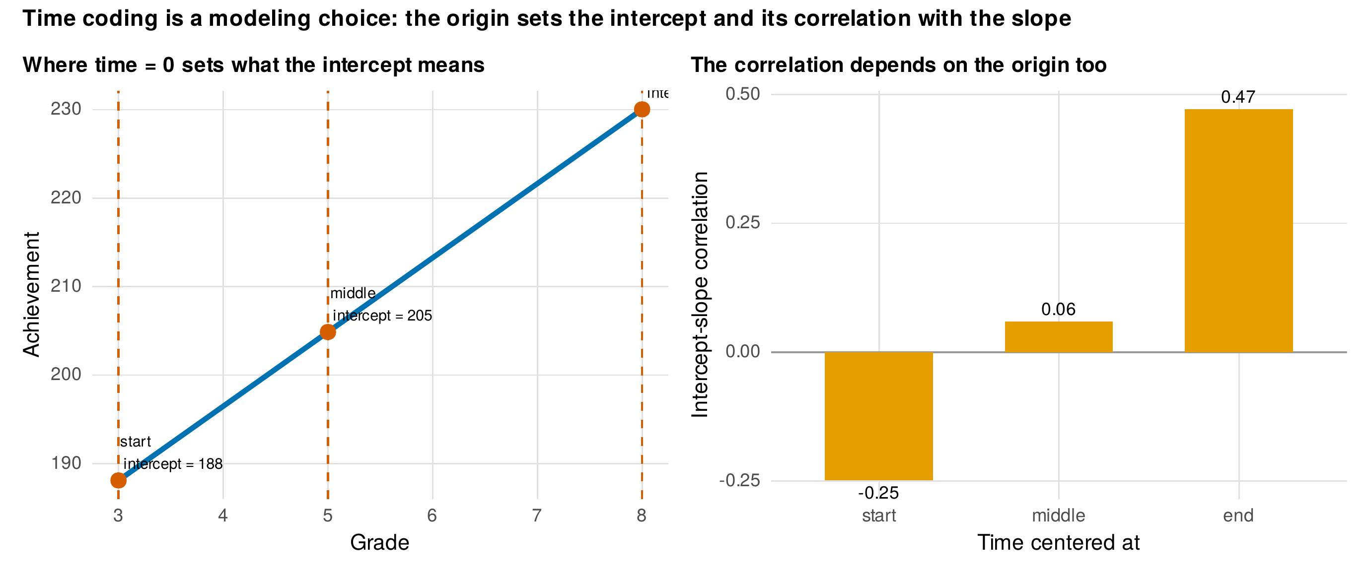
Note. Left: the average linear trajectory of the school-growth data, with three candidate origins marked and the intercept each implies. The slope is the same line regardless of origin. Right: the estimated intercept-slope correlation from the identical model fitted with the origin at the start, the middle, and the end of the window. The correlation moves from \(-0.25\) to \(+0.06\) to \(+0.47\) as the origin shifts later, although the data and the slope are unchanged.
The reversal of the correlation’s sign is not a paradox and not an artifact to be corrected; it is a correct statement that different questions have different answers. The correlation of the slope with the grade-three intercept asks whether children who start school higher gain faster, and the answer is no, they gain slightly slower. The correlation of the slope with the grade-eight intercept asks whether children who end higher got there by gaining faster, and the answer is yes, necessarily, because ending high after a common start requires a steep climb. Both are true of the same children. The practical lesson is that the origin must be chosen so that the intercept is the quantity of scientific interest, most often the start of treatment, the beginning of a developmental window, or a meaningful anchor age, and that the reported intercept variance and intercept-slope correlation must always be interpreted relative to that chosen origin. A reader who encounters a strong intercept-slope correlation in a published growth model should ask where time was set to zero before drawing any substantive conclusion, because the same study centered elsewhere would report a different number. Table 14.2 organizes the origin decision around the question the intercept is meant to answer, together with the metric choice, wave number, elapsed time, or age, that the design and the estimand dictate.
Table 14.2. A decision guide for the time metric and its origin.
| Question or anchor | Time coding | Consequence for the intercept |
|---|---|---|
| Level at the start of observation | Center at the first occasion | Intercept is the baseline level |
| Level at the end or at attainment | Center at the last occasion | Intercept is the final status |
| Level at a substantive event | Center at the event time | Intercept is the level at the event |
| A developmental process indexed by age | Age as the metric (accelerated design) | Requires a cohort-convergence check |
| Persons measured off schedule | Observed time, not wave number | Removes bias from schedule drift |
Note. The origin is chosen so that the intercept is the quantity of scientific interest, because the intercept variance and the intercept-slope correlation are interpretable only relative to it. Recoding the origin changes those quantities but not the model’s fit or its slope, and the metric should be the observed time of each measurement when schedules drift from their nominal dates.
Foundations Box • Why the slope is invariant but the intercept is not
Write the trajectory at a shifted origin \(a^{\ast} = a - c\). The line \(\pi_{0i} + \pi_{1i}a\) becomes \(\pi_{0i} + \pi_{1i}(a^{\ast}+c) = (\pi_{0i}+\pi_{1i}c) + \pi_{1i}a^{\ast}\). The new slope is still \(\pi_{1i}\), so the slope and its variance \(\tau_{11}\) do not change. The new intercept is \(\pi_{0i}^{\ast} = \pi_{0i} + c\,\pi_{1i}\), a linear combination of the old intercept and the slope. Its variance is therefore \(\tau_{00}^{\ast} = \tau_{00} + 2c\,\tau_{01} + c^{2}\tau_{11}\), and its covariance with the slope is \(\tau_{01}^{\ast} = \tau_{01} + c\,\tau_{11}\). The covariance is a straight line in the shift \(c\) with slope \(\tau_{11}>0\), so as the origin moves later the intercept-slope covariance increases without bound and must cross zero exactly once, at \(c = -\tau_{01}/\tau_{11}\). This single algebraic fact generates the entire pattern of Figure 14.1: the sign of the intercept-slope correlation is not a property of the data alone but of the data together with the chosen origin.
14.2 The Shape of Change: Nonlinear Trajectories
Straight-line growth is a strong assumption, and much change in psychology and education is curved: gains that decelerate as a ceiling nears, spurts that follow a lull, or a rate that shifts at a known transition such as school entry or the onset of treatment. The mixed model accommodates curvature without leaving the framework, because a nonlinear trajectory in time can be a linear model in transformed time predictors. Three approaches cover most applications, and they trade smoothness against interpretability in different ways (Cudeck & Harring, 2007; Grimm et al., 2011).
The polynomial growth model adds powers of time as predictors. A quadratic model, \(y_{it} = \gamma_{00} + \gamma_{10}a_{it} + \gamma_{20}a_{it}^{2} + u_{0i} + u_{1i}a_{it} + e_{it}\), introduces a fixed curvature \(\gamma_{20}\) that bends the average trajectory, negative for deceleration and positive for acceleration, and a cubic term adds an inflection. Polynomials are attractive because they remain linear in the parameters, so ordinary mixed-model software fits them, but they carry two liabilities: the coefficients past the linear term have no direct interpretation as a rate, and the fitted curve extrapolates wildly outside the observed range, so a quadratic must never be read beyond the data. On the school-growth means, shown in Figure 14.2, the quadratic term is \(-0.57\), a gentle deceleration, and it earns its place: the Akaike information criterion falls from \(39{,}058\) for the linear model to \(39{,}003\) for the quadratic, a difference of \(54\) that decisively favors the curve, while the cubic term does not improve on the quadratic, its AIC of \(39{,}010\) being slightly worse. The deceleration is real but modest, the kind of tapering common when an achievement measure compresses at its upper end.
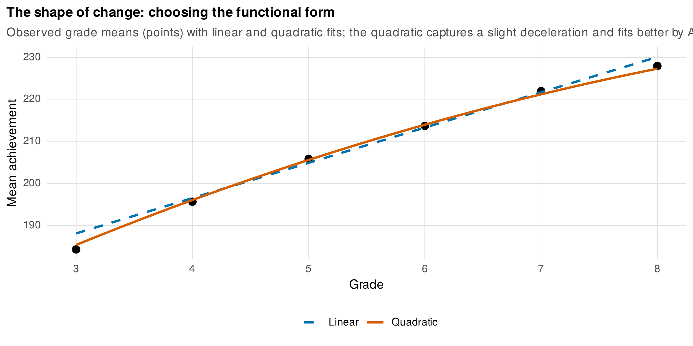
Note. Observed grade means of the school-growth data (points) with the fitted linear (dashed) and quadratic (solid) average trajectories. The quadratic captures a slight deceleration across grades and improves the Akaike information criterion by \(54\) over the linear model; a cubic term adds nothing. Polynomial fits should never be extrapolated beyond the observed grade range.
The piecewise-linear or spline growth model replaces a single line with two or more line segments joined at a knot, a value of time at which the slope is permitted to change. When the knot is placed at a substantively meaningful transition, this model has the interpretive advantage the polynomial lacks: each segment has a slope that is a rate of change in the outcome’s own units. The basis is the time variable together with its positive part beyond the knot, so with a knot at grade six the two predictors are \(a_{it}\) and \((\text{grade}-6)_{+}\), the latter equal to zero before grade six and to grade minus six after it. The coefficient on the first is the pre-knot slope, and the coefficient on the second is the change in slope at the knot, so the post-knot slope is their sum. Fitting this to the school-growth data, shown in Figure 14.3, gives a pre-knot slope of \(9.21\) points per grade, a change of \(-2.48\) at the knot, and hence a post-knot slope of \(6.73\): growth is brisk in the early grades and decelerates in the later ones, the same story the quadratic told but now expressed as two interpretable rates rather than a curvature coefficient. The knot may be fixed a priori from theory, as here, or in more advanced treatments estimated from the data, and the segments may themselves be allowed to vary randomly across persons so that individuals differ in their pre-knot and post-knot rates.
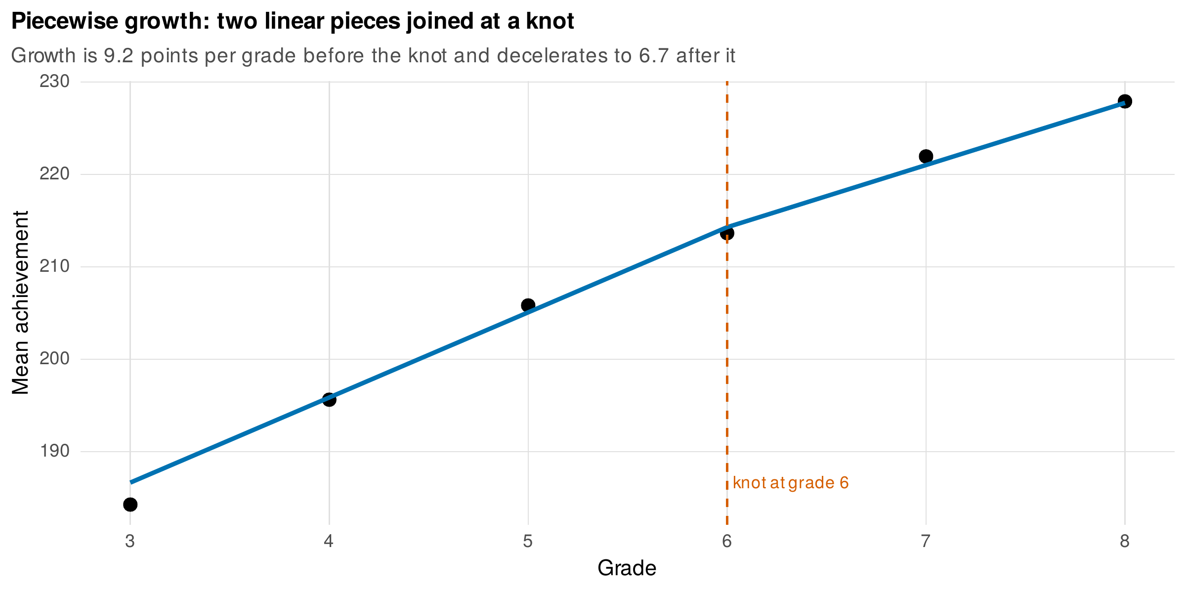
Note. The school-growth means fitted by two linear segments joined at a knot at grade six. The pre-knot slope is \(9.2\) points per grade and the post-knot slope is \(6.7\), a deceleration of \(2.5\) points at the transition. Unlike a polynomial coefficient, each segment slope is a rate of change in the outcome’s own units, which is the interpretive advantage of the spline when the knot marks a meaningful transition.
The choice among shapes is guided by theory first and fit second. If a substantive transition is known, the piecewise model tests it directly and reports rates on both sides. If change is smoothly curved with no natural breakpoint, a low-order polynomial is parsimonious. If the shape is genuinely unknown and the occasions are many, a more flexible spline with several knots, or a nonlinear model with parameters such as an asymptote and a rate, may be warranted, at the cost of interpretability and identification. Fit indices such as the AIC and the Bayesian information criterion adjudicate among nested and non-nested alternatives, but they should never override a functional form that a theory of the process demands, and an extrapolation-prone polynomial chosen only because it fit slightly better is a common and avoidable error. Table 14.3 collects the common forms with their R specifications, the meaning of their parameters, and the conditions under which each is preferred.
Table 14.3. A menu of functional forms for the growth trajectory.
| Form | R specification | Parameter meaning | When preferred |
|---|---|---|---|
| Linear | y ~ t | Constant rate of change | Three waves; monotone change |
| Quadratic | poly(t, 2) | Curvature; deceleration or acceleration | Smooth curve, read only in range |
| Piecewise | pre + post | A rate per segment | A known transition or knot |
| Spline | ns(t, knots) | Flexible local shape | Many waves, unknown shape |
| Nonlinear | nlme(...) | Asymptote and rate constant | Theory supplies the parameters |
Note. Theory selects the form and fit adjudicates among candidates. A polynomial is never read beyond the observed range, and an intrinsically nonlinear form is preferred when its parameters, such as an asymptote or a rate constant, are the substantive quantities of interest. The penalized and intrinsically nonlinear forms are developed in Chapter 30.
14.3 Individually Varying Occasions and the Accelerated Design
A hidden assumption of the balanced growth model is that everyone is measured on the same schedule, so that occasion and time coincide. Real studies routinely violate this. Participants are measured at different chronological ages, assessments drift from their nominal dates, and, most usefully, studies are deliberately designed so that different cohorts cover different but overlapping stretches of the age range. The mixed-model formulation handles all of these without special machinery, because time enters as the numeric predictor \(a_{it}\), which may take a different value for every person on every occasion. This is the decisive practical advantage of the multilevel growth model over the classical repeated-measures analysis of variance of Chapter 11 and, in its balanced form, over the wide-format latent growth model of Chapter 19: individually varying occasions require nothing beyond entering each person’s actual time values (Mehta & West, 2000; Sterba, 2014).
The design that exploits this most powerfully is the accelerated longitudinal design, also called the cohort-sequential design, introduced by Bell (1953) as a way to span a long developmental range in a short calendar time. Instead of following one cohort across the entire age range, which would take as many years as the range is wide, the researcher recruits several cohorts of different ages and follows each for a shorter overlapping period, then links them on the age metric into a single trajectory. In the school-growth data the three cohorts illustrate the design exactly: cohort A is observed in grades three through six, cohort B in grades four through seven, and cohort C in grades five through eight, so that each child contributes only four of the six grades, but the cohorts overlap and together cover the full span. Figure 14.4 shows the three cohort means plotted on the shared grade axis; where the cohorts overlap they nearly coincide, and the single growth model fitted to the pooled data recovers one continuous trajectory across grades three through eight even though no child was measured across all six.
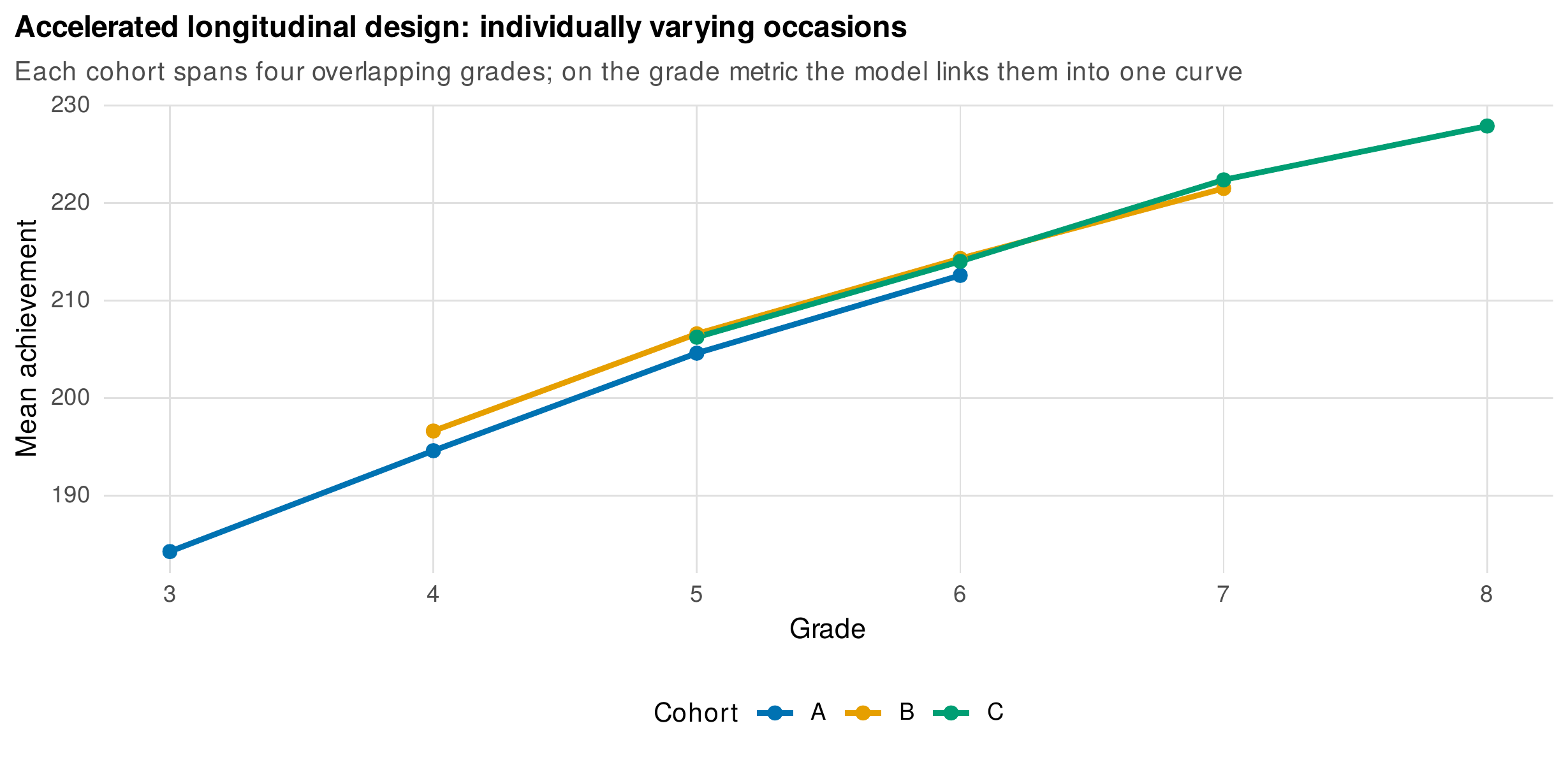
Note. Mean achievement of the three school-growth cohorts plotted on the shared grade metric. Cohort A spans grades three to six, cohort B grades four to seven, and cohort C grades five to eight, so no child is observed across the full range, yet the overlapping segments align and the pooled growth model links them into one trajectory from grade three to grade eight. The linkage rests on the convergence assumption that cohort and age are not confounded.
The power of the design rests on an assumption that must be stated and, where possible, tested. The convergence assumption is that the cohorts are drawn from the same growth process, so that the trajectory depends on age but not on cohort, and the segments contributed by different cohorts can be treated as pieces of one curve rather than as separate curves that happen to overlap (Miyazaki & Raudenbush, 2000; Raudenbush & Chan, 1992). When it holds, the design buys a wide developmental range at a fraction of the calendar time and the participant burden. When it fails, because a secular trend, a cohort-specific event, or differential selection makes the cohorts genuinely different, the linked trajectory is a blend of age change and cohort difference and can misrepresent both. The assumption is checked by adding cohort as a predictor and testing whether it moderates the growth parameters, or by comparing the segments in their overlapping region, and it is defended substantively by arguing that the cohorts differ only in age and not in any factor that would alter the developmental process. The design is a genuine gift of the mixed-model framework, but the linkage it performs is an inference, not a measurement, and honest reporting states the convergence assumption explicitly.
14.4 Conditional Growth: Predicting the Trajectory
The unconditional model describes how people change; the conditional growth model explains why they differ, by admitting person-level covariates as predictors of the growth parameters. A time-invariant covariate \(W_i\), a person characteristic such as treatment arm, sex, or a baseline score, enters the level-two equations for both the intercept and the slope, \(\pi_{0i} = \gamma_{00} + \gamma_{01}W_i + u_{0i}\) and \(\pi_{1i} = \gamma_{10} + \gamma_{11}W_i + u_{1i}\). Substituting into the level-one model produces the combined form \(y_{it} = \gamma_{00} + \gamma_{10}a_{it} + \gamma_{01}W_i + \gamma_{11}W_i a_{it} + u_{0i} + u_{1i}a_{it} + e_{it}\), in which the coefficient \(\gamma_{01}\) is the effect of the covariate on the starting level and, crucially, \(\gamma_{11}\) is the coefficient on the product \(W_i a_{it}\), a cross-level interaction between the person-level covariate and time. This interaction is the formal expression of a covariate that moderates change: it is the amount by which the growth rate differs per unit of the covariate, and it is the quantity that a longitudinal intervention study exists to estimate, because it is the difference in slopes between conditions.
The demonstration uses therapy_rct, the simulated antidepressant trial in which patients in a treatment and a control arm are measured on the Hamilton depression scale over twelve weekly occasions. Fitting the conditional model with arm as the covariate gives a control-arm slope of \(\gamma_{10} = -0.64\) points per week, the improvement patients show under the control condition, and an arm-by-week interaction of \(\gamma_{11} = -0.51\), so that the treatment arm improves at \(-0.64 + (-0.51) = -1.15\) points per week, nearly twice as fast. Figure 14.5 plots the two model-implied trajectories, whose diverging descent is the visual signature of the cross-level interaction. The treatment effect in a growth model is not a difference in means at a single occasion but this difference in slopes, the difference in the rate of change, which is the appropriate estimand for a study of whether an intervention alters a trajectory rather than merely shifting a level. Reporting the interaction coefficient with its confidence interval, and translating it into the implied difference in outcome at the end of the study, communicates the effect in the terms a clinician needs.
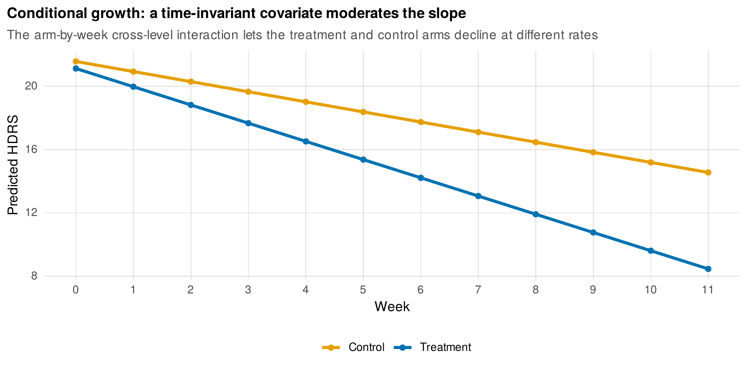
Note. Model-implied trajectories on the Hamilton depression scale for the treatment and control arms of the simulated trial. The control arm declines at \(0.64\) points per week and the treatment arm at \(1.15\), and the gap between the lines is the arm-by-week cross-level interaction of \(-0.51\). In a growth model the treatment effect is this difference in slopes, not a difference in level at any single week.
A conditional model that adds a covariate to the slope also changes the meaning of the slope variance. The unconditional slope variance \(\tau_{11}\) described the total spread of growth rates across all people; once the covariate enters, the residual slope variance describes only the spread that the covariate leaves unexplained. A treatment that strongly moderates growth will absorb a portion of the slope variance, and comparing the residual slope variance before and after adding the covariate quantifies how much of the individual differences in change the covariate accounts for, the growth-model analogue of the variance-explained logic of Chapter 13. Reporting only the interaction coefficient, without noting what it does to the slope variance, tells half the story.
14.5 Time-Varying Covariates in Growth Models
Some predictors change within a person over the course of the study: a fluctuating stressor, a time-varying dose, an evolving context. A time-varying covariate \(x_{it}\) enters at level one alongside time, and its inclusion revives in full the centering problem of Chapter 13, because the raw coefficient on a time-varying covariate confounds two distinct effects. The within-person effect asks whether, when a person’s covariate is higher than that person’s own average, the outcome is correspondingly higher, a question about coupling over time within an individual. The between-person effect asks whether people with higher average levels of the covariate have higher outcomes, a question about stable individual differences. These are different questions with potentially different, even oppositely signed, answers, and the raw coefficient is an uninterpretable blend of them. The resolution is the same person-mean centering developed in Chapter 13: decompose the covariate into a person mean \(\bar{x}_i\) and a within-person deviation \(x_{it}-\bar{x}_i\), and enter both, so that the deviation carries the within-person effect and the person mean carries the between-person effect.
A known-truth simulation makes the recovery visible. Data were generated for \(300\) persons over six occasions from a linear growth process with a genuine within-person covariate effect of \(1.5\) and a distinct, weaker between-person association built in through a shared trait. Fitting the growth model with the covariate entered raw would return a single coefficient contaminated by both. Fitting it with person-mean centering, shown in Figure 14.6, recovers a within-person coefficient of \(1.42\), close to the true \(1.5\), and a separate between-person coefficient of \(0.44\), correctly identifying the within-person effect as the stronger of the two and keeping the two effects apart. The lesson transfers directly from Chapter 13 to the growth setting: a time-varying covariate is a level-one predictor like any other, and the decision to center it by the person mean is the decision about which question its coefficient answers. In growth models the stakes are heightened because time and the time-varying covariate may themselves be correlated, so that a covariate trending with time can steal variance from the growth slope unless the within and between components are separated.
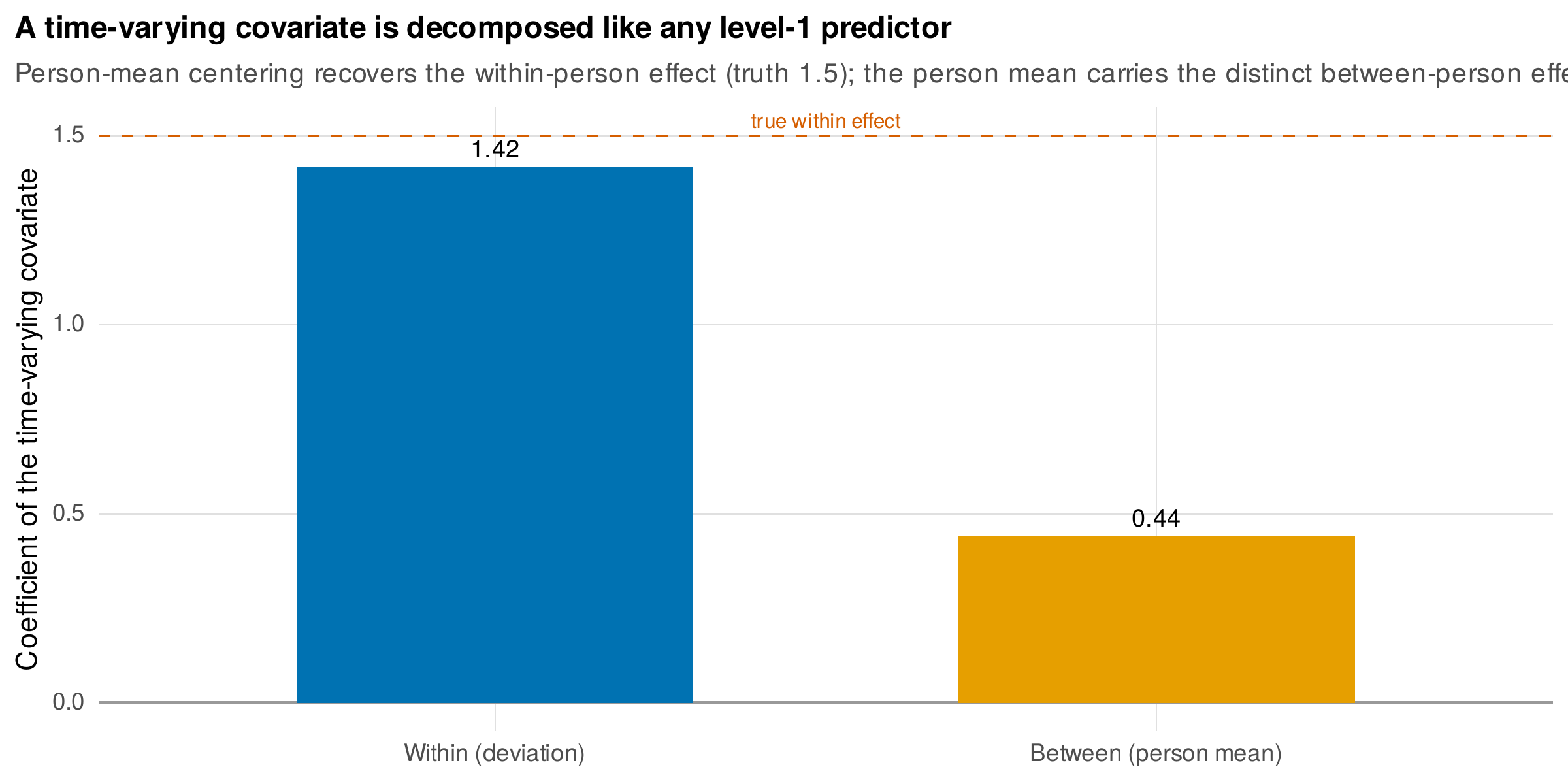
Note. Estimated coefficients of a time-varying covariate in a growth model fitted with person-mean centering, from a simulation whose true within-person effect is \(1.5\) (dashed line). The within-person deviation recovers the effect at \(1.42\); the person mean carries a separate and weaker between-person association of \(0.44\). Entering the covariate raw would blend these two effects into one uninterpretable coefficient.
A time-varying covariate in a growth model raises one complication beyond the within-and-between decomposition, which is that a covariate trending with time competes with the growth slope for the same variance, so a covariate that rises over the study can absorb part of the trajectory and attenuate the estimated rate of change unless it is detrended, ideally within each person (Curran & Bauer, 2011). Table 14.4 lays out the decisions in order.
Table 14.4. Decisions for a time-varying covariate in a growth model.
| Question | Choice | Interpretation |
|---|---|---|
| Within-person or between-person effect wanted? | Person-mean center the covariate | The deviation carries the within-person effect and the person mean the between-person effect |
| Does the covariate trend with time? | Detrend it, per person if needed | Separates the covariate’s effect from the growth slope it would otherwise absorb |
| Entered raw, uncentered | Not recommended | A single blended coefficient that can carry the wrong sign |
Note. A time-varying covariate correlated with time can absorb variance belonging to the growth trajectory, so its within-person and between-person components are separated as in Chapter 13, and a trending covariate is detrended before interpretation. Adding a time-varying covariate also changes the meaning of the growth factors, a subtlety coordinated with the parallel treatment in Chapter 19.
14.6 Residual Covariance Structure
The random effects of a growth model imply a marginal covariance among the repeated measurements, the \(\mathbf{Z}_i\mathbf{T}\mathbf{Z}_i' + \sigma^2\mathbf{I}\) of Chapter 13, but the assumption embedded in the \(\sigma^2\mathbf{I}\) term, that the level-one residuals are independent and equally variable across occasions, is often too strong for closely spaced measurements. When observations near in time are more alike than the random effects alone predict, the leftover dependence lives in the residuals, and modeling it directly can improve both fit and the standard errors of the fixed effects. The tool is a residual covariance structure, a parameterized form for the within-person residual covariance \(\mathbf{R}_i\) that replaces \(\sigma^2\mathbf{I}\), and in R it is supplied by the nlme package, whose correlation argument fits structures that lme4 does not. Three structures span the common cases, illustrated in Figure 14.7. The independent structure is the default \(\sigma^2\mathbf{I}\), with no residual correlation. The first-order autoregressive, AR(1), structure makes the residual correlation decay geometrically with separation, \(\rho^{|s-t|}\), so that adjacent residuals are most alike and distant ones nearly independent, a natural form for equally spaced occasions. The Toeplitz structure, here approximated by a second-order autoregressive form, allows a separate correlation at each lag, a more flexible banded pattern that costs more parameters.
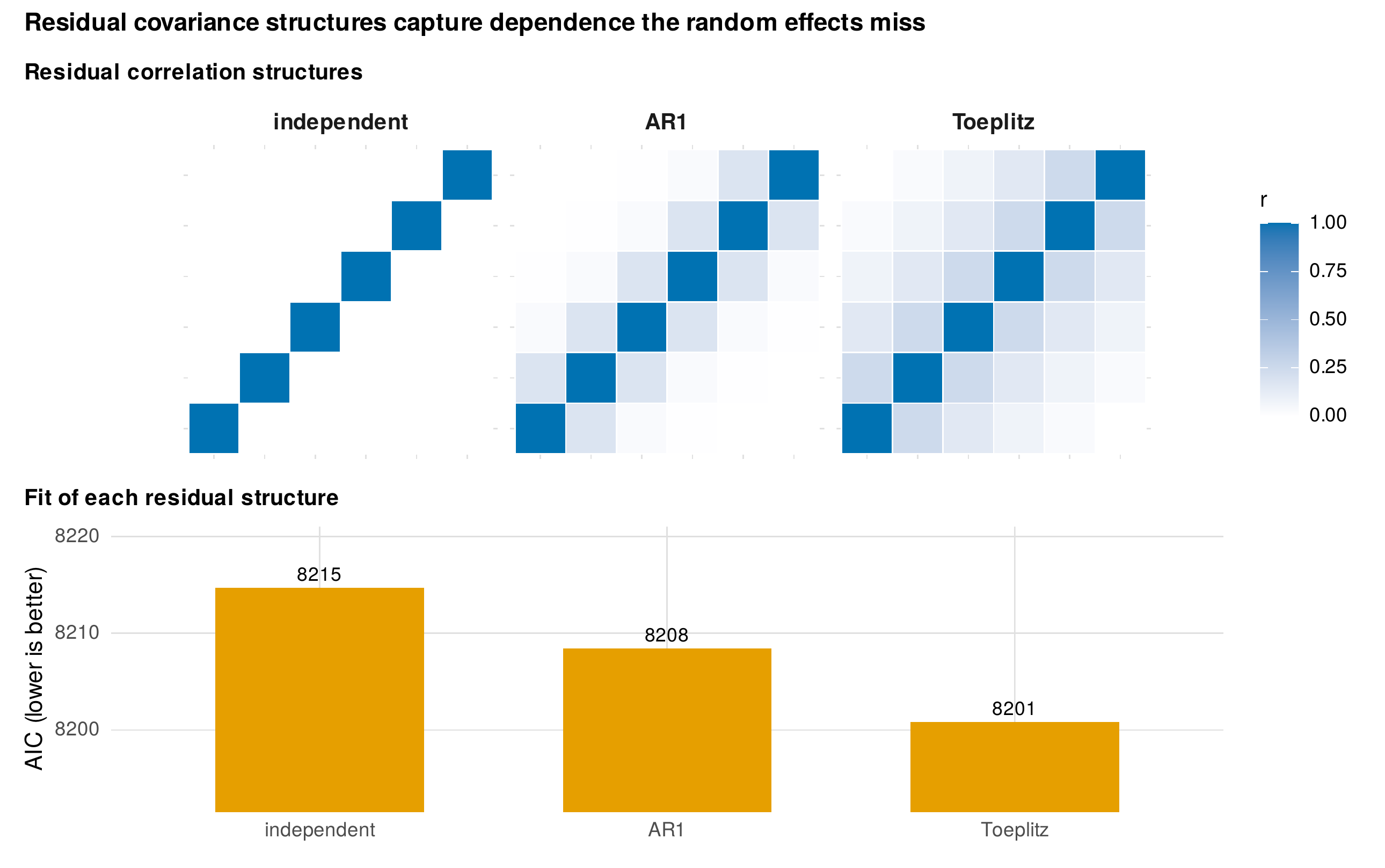
Note. Top: three residual correlation structures for six occasions, shown as heatmaps, the independent structure with no off-diagonal correlation, the AR(1) structure with geometric decay, and a Toeplitz-like structure with a separate correlation at each lag. Bottom: the Akaike information criterion of each structure layered on a random-intercept growth model fitted to a subset of the school-growth data. Lower is better; the AR(1) and Toeplitz structures improve on independence, indicating residual dependence the random intercept did not absorb.
Fitting the three structures on a random-intercept growth model, using a \(250\)-child subset of the school-growth data for speed, orders them as the theory predicts. The independent model has an AIC of \(8{,}215\); adding an AR(1) residual correlation, estimated at \(\rho = 0.18\), lowers it to \(8{,}208\); and the Toeplitz-like structure lowers it further to \(8{,}201\). The improvements are modest here because the random intercept already captures most of the within-child dependence, which is the usual situation: when the random-effect structure is rich, especially with a random slope, there is little residual dependence left to model, and an independent residual is adequate. Residual covariance modeling earns its keep in the opposite case, when the random structure is deliberately kept simple, when occasions are numerous and closely spaced as in intensive longitudinal designs, or when the residual autocorrelation is itself of interest. The two approaches to within-person dependence, richer random effects and structured residuals, are partly substitutable, and a well-specified model uses whichever matches the mechanism: random slopes for genuine individual differences in trajectory, structured residuals for serial dependence in the measurement process. Comparing structures by information criteria, as here, is the practical way to decide, with the caveat that the comparison must hold the fixed effects and the random effects constant and vary only the residual structure. Table 14.5 lists the structures the nlme package supplies and the designs each suits.
Table 14.5. Level-one residual covariance structures in nlme.
| Structure | nlme argument | Plausible design |
|---|---|---|
| Independent | Default residual | Random effects already capture the dependence |
| First-order autoregressive | correlation = corAR1() | Equally spaced occasions with serial decay |
| Toeplitz or ARMA | correlation = corARMA(p, q) | Banded dependence with distinct correlations by lag |
| Heterogeneous variance | weights = varIdent() | Residual variance changing across occasions |
Note. A structured residual and a random slope both produce autocorrelation that rises toward the diagonal, so the two can be difficult to separate; a rich random-effect structure is the first recourse, and the residual structure is chosen by information criteria with the fixed and random effects held constant and reported as a sensitivity check.
In Practice • random slopes or structured residuals?
Faced with within-person dependence, a modeler can add a random slope or add a structured residual, and the two are easy to confuse because both improve fit. The distinction is mechanistic. A random slope says people genuinely differ in their rate of change, a between-person fact, and it implies a specific marginal covariance whose variance grows with time. A structured residual says the measurement errors are serially correlated, a within-person fact about the noise process, and it implies a covariance whose correlations decay with lag but whose variance is roughly constant. When both are plausible and the data are rich, fit both and let an information criterion and the substantive interpretation decide; when the data are thin, prefer the random slope if individual differences in change are the scientific question, and the structured residual if the dependence is a nuisance in the measurement to be controlled rather than explained. Fitting an elaborate residual structure on top of a full random-slope model often produces a singular or non-identified fit, because the two are competing to explain the same dependence.
14.7 Worked Example and Reporting
A complete growth analysis of the school-growth achievement data proceeds by the model-building sequence of Chapter 13, specialized to growth. The unconditional means model, with only a random intercept and no time, partitions the total variance and confirms that a substantial share lies between children and between schools, justifying the multilevel treatment. The unconditional growth model adds time as a fixed and random effect, establishing that achievement rises on average by \(8.4\) points per grade and, through a slope standard deviation of \(3.1\), that children differ meaningfully in their rates. The shape is then examined: the quadratic term improves fit decisively over the linear, indicating a mild deceleration, so the reported model carries a fixed quadratic term. Figure 14.8 shows the fitted quadratic model over a sample of individual trajectories and, alongside, the model-implied grade means against the observed means, the growth-model diagnostic that asks whether the chosen functional form reproduces the average trajectory. The implied and observed means coincide closely across all six grades, evidence that the quadratic captures the mean structure. A conditional model would then add school-level and child-level covariates to explain the intercept and slope variances, and the residual structure would be checked, though here the random slope leaves little residual dependence to model.
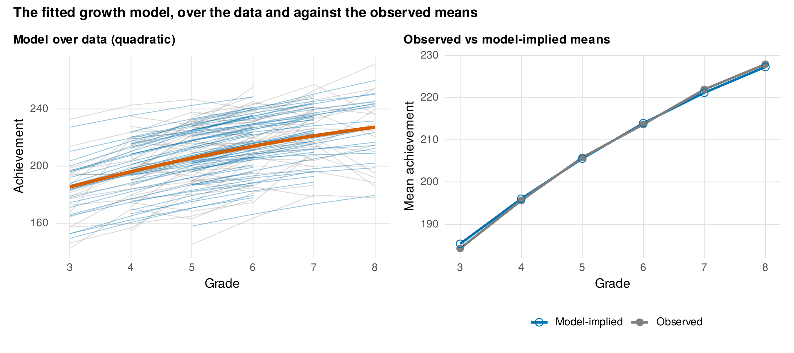
Note. Left: the fitted quadratic average trajectory (red) over a sample of \(60\) individual child trajectories (grey) and their model-implied fits (blue), on the school-growth data. Right: the model-implied grade means (blue) against the observed grade means (grey); their close agreement across grades three to eight indicates that the quadratic functional form reproduces the mean structure of the data.
Reporting a growth model to publication standard requires several elements that a cross-sectional write-up does not. The time metric and its origin must be stated explicitly, because every intercept-related quantity depends on them, and the reader cannot interpret an intercept variance or an intercept-slope correlation without knowing where time is zero. The functional form must be named and justified, with the fit comparison that led to it, and any nonlinear coefficient translated into a substantive statement about deceleration or acceleration rather than left as a bare number. The fixed effects give the average trajectory and, in a conditional model, the covariate effects on level and on slope, the latter being the cross-level interactions that carry the substantive moderation. The random effects, the intercept and slope variances and their correlation, are reported as the description of individual differences in change, with the correlation interpreted relative to the stated origin. Missing data handling should be described, since the likelihood-based mixed model uses all available occasions under the missing-at-random assumption developed in Chapter 6, a major advantage over listwise-deletion alternatives. Curran, Obeidat, and Losardo (2010) provide a lucid catalogue of the questions that recur in growth modeling and the reporting decisions each entails, and Grimm, Ram, and Estabrook (2017) give the fuller treatment that connects the multilevel form used here to the structural-equation form of Chapter 19. Table 14.6 consolidates the elements a growth-model write-up must contain beyond an ordinary regression report.
Table 14.6. A reporting checklist for a growth-curve analysis.
| Element | What to report |
|---|---|
| Time metric and origin | The variable, its units, and where it equals zero |
| Functional form | The shape and the basis on which it was selected |
| Fixed effects | The average trajectory and any covariate effects on level and on slope |
| Random effects | The intercept and slope variances and their correlation, interpreted at the stated origin |
| Residual structure | Independent or structured, with a sensitivity note |
| Missing data | The assumed mechanism and the estimator, typically full-information maximum likelihood |
| Model comparison | The information criteria or likelihood-ratio tests behind the shape and predictor choices |
Note. The elements a growth-model write-up must include beyond an ordinary regression report, extending the mixed-model checklist of Chapter 13. Every intercept-related quantity is uninterpretable without the time metric and origin, which are therefore stated first.
14.8 Running the Growth Model in R
The unconditional and conditional growth models are fitted with lmer from lme4, with time entered as a numeric predictor and centered at the chosen origin. The shape comparisons and the accelerated linkage require nothing beyond ordinary model syntax, because time is just a covariate.
library(lme4); library(lmerTest); library(dplyr)
sg <- readRDS("Examples/data/school_growth.rds") |>
  mutate(grade_c = grade - 3)                       # origin at grade 3

# --- Unconditional linear growth ---
m_lin <- lmer(achievement ~ grade_c + (1 + grade_c | child_id) +
                (1 | school_id), sg)
summary(m_lin); VarCorr(m_lin)                       # fixed slope; T matrix

# --- Shape: polynomial vs linear (compare by AIC under ML) ---
m_quad <- lmer(achievement ~ poly(grade_c, 2, raw = TRUE) +
                 (1 + grade_c | child_id) + (1 | school_id), sg, REML = FALSE)
AIC(update(m_lin, REML = FALSE), m_quad)

# --- Shape: piecewise with a knot at grade 6 ---
sg <- sg |> mutate(pre = grade_c, post = pmax(grade - 6, 0))
m_pw <- lmer(achievement ~ pre + post + (1 + pre | child_id) +
               (1 | school_id), sg)                  # post = change in slope
The origin is changed simply by recoding the time variable, and re-fitting shows the intercept, its variance, and its correlation with the slope moving while the slope stays fixed. A conditional model adds a person-level covariate to the slope through an interaction with time, and a time-varying covariate is person-mean centered exactly as in Chapter 13.
# --- Origin changes the intercept and the intercept-slope correlation ---
for (c0 in c(3, 5, 8)) {
  d <- sg |> mutate(gt = grade - c0)
  print(VarCorr(lmer(achievement ~ gt + (1 + gt | child_id) +
                       (1 | school_id), d)))
}

# --- Conditional growth: cross-level interaction (treatment trial) ---
rct <- readRDS("Examples/data/therapy_rct.rds")
m_cond <- lmer(hdrs ~ week * arm + (1 + week | patient_id), rct)  # week:arm = slope difference

# --- Residual covariance structure needs nlme, not lme4 ---
library(nlme)
g0 <- lme(achievement ~ grade_c, random = ~1 | child_id, data = sg, method = "ML")
g1 <- update(g0, correlation = corAR1(form = ~ grade | child_id))  # AR(1) residuals
anova(g0, g1)                                                       # compare by AIC/LRT
The complete analysis, including the time-coding demonstration, the polynomial and piecewise fits, the accelerated-cohort means, the conditional and time-varying-covariate models, and the residual-structure comparison, is the shipped script ch14_analysis_V01.R, with figures drawn by ch14_figures_V01.R. The nlme package is required for the residual structures, and the structural-equation parameterization of the same growth models, taken up in Chapter 19, is fitted in lavaan.
Software Note • the same growth model across programs
The multilevel growth model is fitted by MIXED in SPSS, mixed in Stata, PROC MIXED in SAS, and TYPE = TWOLEVEL or the growth command in Mplus, and each accepts individually varying time values, so the accelerated design is fitted the same way in all of them. Two cross-program cautions specific to growth models matter. First, the residual covariance structures of Section 14.6 are named differently, corAR1 in nlme, REPEATED with a covariance type in SAS and SPSS, and the residual options in Stata, and the default is independence everywhere, so a structured residual must be requested deliberately. Second, the structural-equation programs fit growth as a latent curve model in wide format, which requires balanced or explicitly patterned occasions and handles individually varying times through definition variables or the TSCORES option; the multilevel long-format fit used in this chapter imposes no such requirement, which is why it is preferred when occasions vary freely across persons.
14.9 Common Misconceptions
Several beliefs about growth models mislead. The first is that the intercept-slope correlation is a fixed property of the data; it is a property of the data and the chosen origin together, and it changes, up to reversing its sign, as the origin moves (Figure 14.1), so it is meaningless without a stated time zero. The second is that a better-fitting polynomial is a better model; a polynomial that fits marginally better may extrapolate absurdly and lacks interpretable coefficients, and a theory-driven piecewise or nonlinear form is often preferable even at equal fit. The third is that an accelerated design measures a long trajectory; it infers one, under the convergence assumption that cohorts differ only in age, and when that assumption fails the linked curve confounds development with cohort. The fourth is that the coefficient of a time-varying covariate is its effect; without person-mean centering it is an uninterpretable blend of a within-person and a between-person effect that can carry the wrong sign. The fifth is that structured residuals and random slopes are interchangeable fixes for dependence; they encode different mechanisms, individual differences in change versus serial correlation in the measurement, and fitting both in full often yields a singular model.
Common Pitfall • four errors in growth-model practice
First, reporting an intercept variance or intercept-slope correlation without stating the origin: every intercept-related quantity depends on where time is zero, so the origin must be named and chosen to make the intercept the quantity of interest. Second, extrapolating a polynomial beyond the data: a quadratic or cubic fitted within the observed range says nothing credible outside it and should never be projected forward. Third, linking cohorts in an accelerated design without checking convergence: add cohort as a moderator of the growth parameters and defend the assumption that cohorts differ only in age before treating the segments as one curve. Fourth, entering a time-varying covariate raw: person-mean center it and report the within-person and between-person effects separately, as in Chapter 13.
Chapter Summary
The growth curve model is the linear mixed model of Chapter 13 with time as the level-one predictor, so its estimation, inference, and centering logic all carry over unchanged. The person-specific intercept and slope become a starting level and a rate of change, and the random-effect covariance, the intercept variance, the slope variance, and their correlation, is the empirical description of individual differences in change. The origin of the time metric is a consequential modeling choice: it fixes the meaning of the intercept and, through the algebra of a shifted line, determines the intercept variance and the intercept-slope correlation, which can reverse sign as the origin moves while the slope stays invariant (Figure 14.1). Nonlinear change is modeled by polynomial, piecewise-linear, or spline bases, trading smoothness against the interpretability of a segment slope (Figures 14.2 and 14.3); on the school-growth data a quadratic and a two-piece spline both capture a mild deceleration. Individually varying occasions require nothing beyond entering each person’s actual time values, which makes the accelerated longitudinal design possible, linking overlapping cohorts into one trajectory under the convergence assumption (Figure 14.4). Person-level covariates enter as predictors of the intercept and slope, and a covariate on the slope is a cross-level interaction with time, the estimand of a longitudinal intervention study (Figure 14.5). A time-varying covariate is decomposed by person-mean centering into within-person and between-person effects (Figure 14.6). Residual dependence the random effects leave behind is modeled by AR(1) or Toeplitz residual structures in nlme, which help most when the random structure is deliberately simple (Figure 14.7). A complete analysis states the time metric, justifies the shape, and reports both the average trajectory and the individual differences (Figure 14.8).
Where to Go Next
The growth model developed here is extended in several directions. Chapters 15 and 16 carry it to non-normal and non-continuous outcomes through the generalized linear mixed model, so that counts, binary outcomes, and bounded scales can be grown. Chapter 17 supplies Bayesian estimation, which stabilizes the weakly identified random structures that rich growth models often produce and which handles nonlinear growth parameters gracefully. Chapter 19 reveals the latent growth curve model to be this same model in structural-equation form, where the intercept and slope become latent factors, the implied covariance of Section 14.6 becomes a factor structure, and the framework gains the ability to model the growth factors as causes and effects of other variables. Chapters 20 and 21 build on that to the growth mixture model, which asks whether the population contains distinct latent classes of trajectories rather than one trajectory with continuous variation, and to the parallel-process and cross-lagged extensions that model the joint growth of two constructs. The time-coding and centering lessons of this chapter recur throughout, because wherever time is a predictor its origin and its within-and-between decomposition determine what the model’s coefficients mean.
Exercises
- 14.1 Recode the origin. On a provided growth dataset, fit the linear model with time centered at the first, middle, and last occasion, and tabulate the intercept, the intercept variance, and the intercept-slope correlation at each. Verify algebraically that the slope is unchanged and that the covariance moves linearly in the shift, and identify the origin at which the correlation is zero.
- 14.2 Choose a shape. Fit linear, quadratic, and two-piece piecewise models to a curved trajectory, compare them by AIC and BIC, and argue for one on grounds of theory and interpretability, not fit alone. Translate the chosen model’s nonlinear parameter into a substantive statement about the rate of change.
- 14.3 Link the cohorts. On an accelerated design, fit the pooled growth model, then add cohort as a moderator of the intercept and slope and test the convergence assumption. Report whether the cohorts can be treated as one process and what the linked trajectory would misrepresent if they cannot.
- 14.4 Estimate a treatment effect on slope. In a two-arm trial, fit the conditional growth model, report the arm-by-time cross-level interaction with its confidence interval, and translate it into the implied difference in outcome at the end of the study. State what the interaction does to the residual slope variance.
- 14.5 Decompose a time-varying covariate. Enter a time-varying covariate raw and then person-mean centered, and write the three interpretations, identifying which coefficient answers the within-person question and explaining how the raw coefficient blends the two.
- 14.6 Model the residuals. On closely spaced occasions, fit a random-intercept growth model with independent, AR(1), and Toeplitz residual structures in
nlme, compare them by AIC, and discuss whether a random slope would be a better account of the same dependence.
References
Bell, R. Q. (1953). Convergence: An accelerated longitudinal approach. Child Development, 24(2), 145–152. https://doi.org/10.2307/1126345
Biesanz, J. C., Deeb-Sossa, N., Papadakis, A. A., Bollen, K. A., & Curran, P. J. (2004). The role of coding time in estimating and interpreting growth curve models. Psychological Methods, 9(1), 30–52. https://doi.org/10.1037/1082-989X.9.1.30
Bollen, K. A., & Curran, P. J. (2006). Latent curve models: A structural equation perspective. Wiley. https://doi.org/10.1002/0471746096
Cudeck, R., & Harring, J. R. (2007). Analysis of nonlinear patterns of change with random coefficient models. Annual Review of Psychology, 58(1), 615–637. https://doi.org/10.1146/annurev.psych.58.110405.085520
Curran, P. J., & Bauer, D. J. (2011). The disaggregation of within-person and between-person effects in longitudinal models of change. Annual Review of Psychology, 62, 583–619. https://doi.org/10.1146/annurev.psych.093008.100356
Curran, P. J., Obeidat, K., & Losardo, D. (2010). Twelve frequently asked questions about growth curve modeling. Journal of Cognition and Development, 11(2), 121–136. https://doi.org/10.1080/15248371003699969
Grimm, K. J., Ram, N., & Estabrook, R. (2017). Growth modeling: Structural equation and multilevel modeling approaches. Guilford Press.
Grimm, K. J., Ram, N., & Hamagami, F. (2011). Nonlinear growth curves in developmental research. Child Development, 82(5), 1357–1371. https://doi.org/10.1111/j.1467-8624.2011.01630.x
Mehta, P. D., & West, S. G. (2000). Putting the individual back into individual growth curves. Psychological Methods, 5(1), 23–43. https://doi.org/10.1037/1082-989X.5.1.23
Miyazaki, Y., & Raudenbush, S. W. (2000). Tests for linkage of multiple cohorts in an accelerated longitudinal design. Psychological Methods, 5(1), 44–63. https://doi.org/10.1037/1082-989X.5.1.44
Raudenbush, S. W., & Bryk, A. S. (2002). Hierarchical linear models: Applications and data analysis methods (2nd ed.). Sage.
Raudenbush, S. W., & Chan, W.-S. (1992). Growth curve analysis in accelerated longitudinal designs. Journal of Research in Crime and Delinquency, 29(4), 387–411. https://doi.org/10.1177/0022427892029004001
Singer, J. D., & Willett, J. B. (2003). Applied longitudinal data analysis: Modeling change and event occurrence. Oxford University Press. https://doi.org/10.1093/acprof:oso/9780195152968.001.0001
Sterba, S. K. (2014). Fitting nonlinear latent growth curve models with individually varying time points. Structural Equation Modeling: A Multidisciplinary Journal, 21(4), 630–647. https://doi.org/10.1080/10705511.2014.919828