Chapter 15
Generalized Linear Mixed Models for Categorical and Count Outcomes
The linear mixed model of Chapters 13 and 14 assumed a continuous, conditionally normal outcome. Much of what psychology measures repeatedly is not of that kind. A symptom either remits or it does not, a clinician rates severity on an ordered scale, a diary records how many drinks or cigarettes or arguments a day contained, and these outcomes are binary, ordinal, and count. The generalized linear mixed model extends the machinery of Chapter 13 to such outcomes by inserting a link function between the linear predictor and the mean, exactly as the ordinary generalized linear model extends ordinary regression, while keeping the random effects that make the data longitudinal. The extension is mechanically small but interpretively large. Three burdens fall on the analyst that did not arise for continuous outcomes: the coefficients live on a nonlinear scale where a subject-specific effect and a population-averaged effect differ, so interpretation requires the same conditional-versus-marginal discipline that Chapter 12 developed from the other side; the likelihood no longer has a closed form, so estimation rests on an integral approximation whose accuracy must be checked; and count outcomes carry distributional questions, overdispersion and excess zeros, that are not nuisances to be patched but theories about the process that generated the data. This chapter develops each burden with a worked longitudinal example, and it insists throughout that results be reported in quantities a reader can feel, predicted probabilities and rates, not bare odds ratios.
Learning Objectives
After working through this chapter, you should be able to: (1) specify a generalized linear mixed model by its family, link, and random-effects structure for binary, ordinal, and count outcomes; (2) interpret coefficients on their natural scale as subject-specific effects, distinguish them from population-averaged effects, and convert both to predicted probabilities and rates; (3) explain why the likelihood requires an integral approximation, distinguish penalized quasi-likelihood, Laplace, and adaptive Gauss-Hermite quadrature, and recognize when the choice changes the answer; (4) diagnose and model overdispersion through the negative binomial or an observation-level random effect, and excess zeros through zero-inflation or a hurdle, choosing between them on substantive grounds; (5) fit an ordinal cumulative-logit mixed model and check its proportional-odds assumption; (6) validate a fitted model with simulation-based residuals; and (7) report a generalized linear mixed model to publication standard with interpretable predicted quantities.
15.1 From the Linear Mixed Model to the Generalized Linear Mixed Model
The generalized linear mixed model (GLMM) is built from three parts, the same three that define any generalized linear model, with random effects added to the third. The first is a distribution for the outcome from the exponential family, Bernoulli for a binary outcome, multinomial for an ordinal one, Poisson or negative binomial for a count. The second is a link function \(g\) that maps the mean of the outcome onto the whole real line, the logit for probabilities and the log for rates being the canonical choices. The third is a linear predictor that now contains both fixed and random effects, \(g(\mu_{it}) = \eta_{it} = \mathbf{x}_{it}'\bm{\gamma} + \mathbf{z}_{it}'\mathbf{u}_i\), with the random effects \(\mathbf{u}_i \sim N(\mathbf{0}, \mathbf{T})\) exactly as in Chapter 13. For a binary remission outcome measured weekly, the model is \(\text{logit}\,\Pr(y_{it}=1) = \gamma_{00} + \gamma_{10}\,\text{week}_{it} + u_{0i}\), a logistic growth in the log-odds of remission with a person-specific intercept. The mechanics are a small step from the linear mixed model; the interpretation is not. Table 15.1 pairs the common outcome types with their family, link, and R implementation.
Table 15.1. Choosing a family and link by outcome type.
| Outcome | Family | Link | R implementation |
|---|---|---|---|
| Binary | Binomial | Logit | glmer(..., binomial) |
| Ordinal | Cumulative | Logit | clmm (ordinal) |
| Count | Poisson | Log | glmer(..., poisson) |
| Overdispersed count | Negative binomial | Log | glmer.nb; glmmTMB |
| Count, excess zeros | Hurdle or zero-inflated | Log | glmmTMB |
Note. The family encodes the outcome’s distribution and the link maps its mean onto the whole real line. The logit and log links are canonical for probabilities and rates; a probit link, in which the latent residual is normal rather than logistic, is an alternative for binary and ordinal outcomes and connects to the categorical measurement models of Chapter 18.
For binary and ordinal outcomes the model has an illuminating equivalent form as a threshold model on a latent continuous variable. Imagine an unobserved continuous propensity \(y^{\ast}_{it} = \eta_{it} + \varepsilon_{it}\), and suppose the observed category is determined by where this latent variable falls relative to one or more thresholds. A binary outcome has a single threshold: the event occurs when the latent propensity exceeds it. An ordinal outcome with \(K\) categories has \(K-1\) thresholds that carve the latent axis into ordered bands. Figure 15.1 draws both. This construction is not a fiction layered onto the model but the reason logistic and probit links take the form they do: the logit link arises when the latent residual \(\varepsilon\) is assumed standard logistic, the probit when it is assumed standard normal. It also exposes a fact with large consequences, developed below, that the latent residual variance is not estimated but fixed by the choice of link, at \(\pi^2/3\) for the logit.
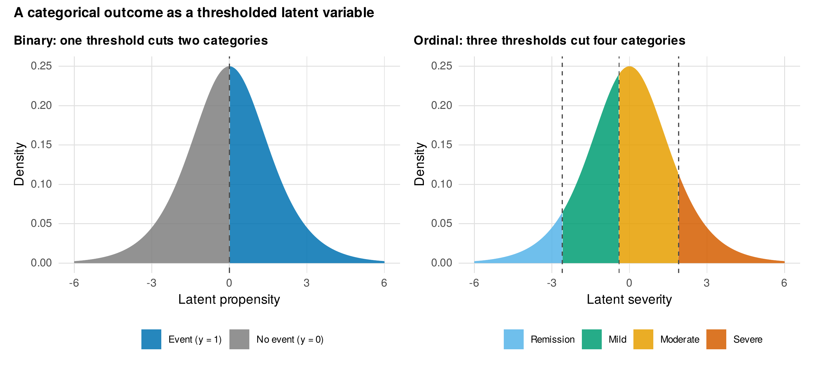
Note. Left: a binary outcome arises when a latent propensity crosses a single threshold, dividing the latent density into no-event and event regions. Right: an ordinal outcome with four categories arises from three thresholds that partition the same latent density into ordered bands. The logit link corresponds to a standard logistic latent residual, whose variance is fixed at \(\pi^2/3\) rather than estimated.
15.1.1 Conditional and Marginal: The Interpretation the Link Forces
Because the link is nonlinear, a coefficient in a GLMM is a subject-specific or conditional effect: it describes the change in the log-odds or log-rate for a given individual, holding that individual’s random effect fixed. This is the mirror image of the population-averaged, marginal effect that the generalized estimating equation of Chapter 12 estimates, and the two are not equal. Averaging a collection of individual logistic curves does not produce a logistic curve with the same slope; it produces a flatter curve, because the nonlinear link does not commute with the expectation over the random effects. The population-averaged effect is therefore attenuated toward zero relative to the subject-specific effect, by a factor that grows with the random-effect variance, and this is precisely the attenuation relation of Chapter 12 seen from the model-based side. Figure 15.2 shows the point on the remission data: the subject-specific curve for a typical patient and the population-averaged curve differ, and neither is a rescaling of the other. In the fitted model the intercept variance is large, with a person standard deviation on the log-odds scale near \(2.7\), so the gap is substantial: at week eight in the treatment arm the model-implied probability of remission for the median patient is \(.05\), while the population-averaged probability across patients is \(.18\).
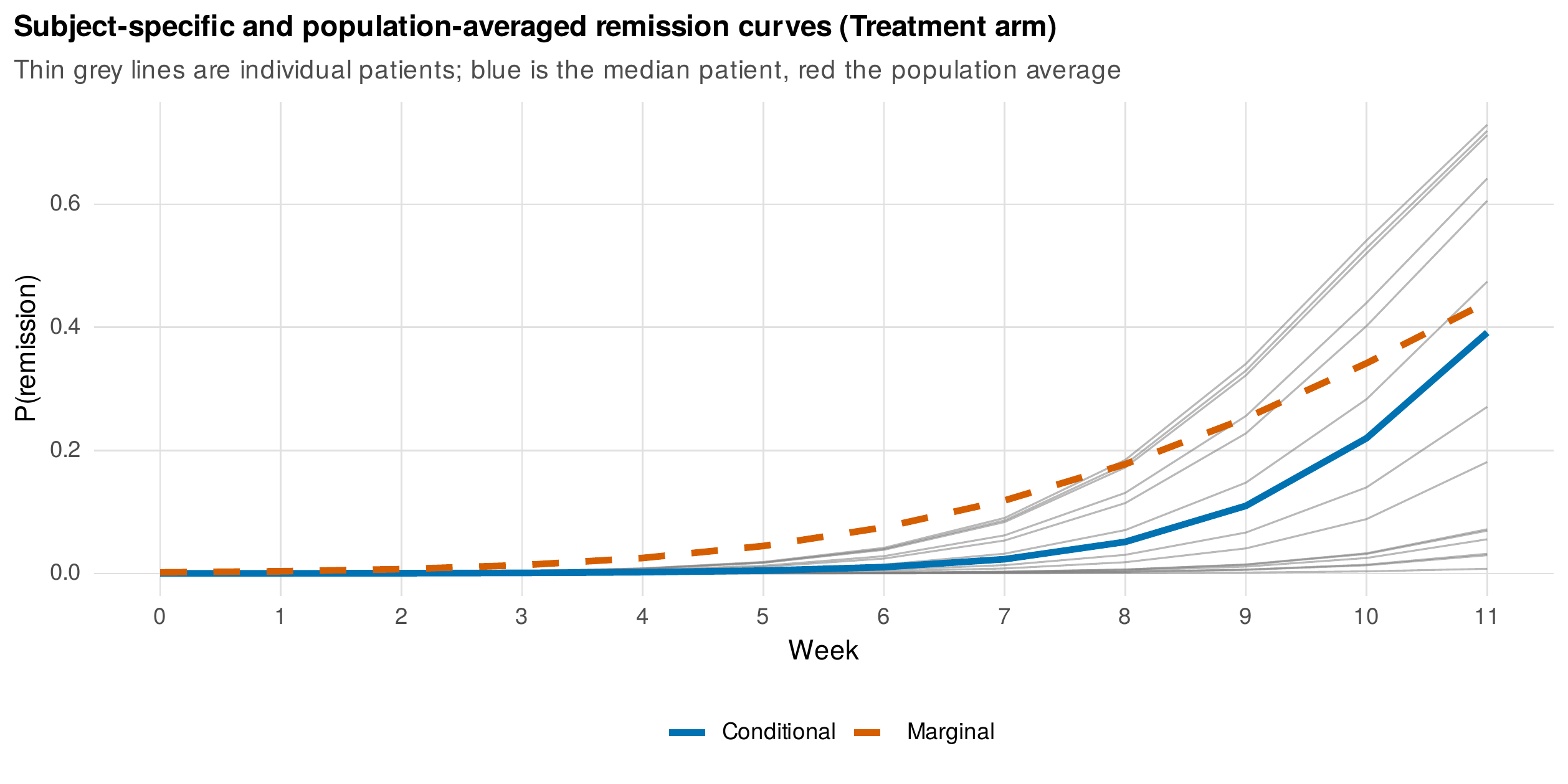
Note. Predicted remission probability over weeks in the treatment arm. Thin grey lines are individual patients implied by the fitted random effects; the blue curve is the subject-specific trajectory of the median patient (random effect zero), and the red dashed curve is the population average across patients. Because the logit link is nonlinear, the average of the individual curves is not the curve of the average patient, and the population-averaged effect of week is attenuated relative to the subject-specific effect. This is the Chapter 12 attenuation seen from the mixed-model side.
Neither quantity is the right one in general; they answer different questions. The subject-specific effect answers how an intervention changes the odds for a particular person, the estimand of most theoretical and clinical interest, while the marginal effect answers how the population prevalence shifts, the estimand of most public-health interest. The requirement is only that the analyst know which one a given number is and report accordingly. A coefficient from a GLMM is subject-specific; if a reviewer asks for a population-averaged effect, it is obtained by averaging the model’s predicted probabilities over the random-effect distribution and over the covariate distribution, a computation that modern tools automate, not by reinterpreting the coefficient in place.
15.1.2 Why Logistic Coefficients Do Not Compare Across Models
The fixed latent residual variance has a consequence that repeatedly misleads. In ordinary linear regression, adding a predictor that is uncorrelated with those already in the model leaves their coefficients essentially unchanged, because the residual variance simply shrinks to absorb the newly explained variation. In logistic regression the residual variance cannot shrink, because it is fixed at \(\pi^2/3\) by the link. When a new predictor explains part of the outcome, the whole latent scale is effectively rescaled, and the coefficients of the other predictors change even when those predictors are uncorrelated with the newcomer (Mood, 2010). Figure 15.3 demonstrates this with a known-truth simulation in which two predictors are independent by construction and the true coefficient of the first is \(1.0\): fitting the outcome on the first predictor alone returns \(0.72\), and adding the second, which is orthogonal to the first, moves the first coefficient to its true \(1.0\). The lesson is that logistic and other GLMM coefficients cannot be compared across nested models, or across groups with different residual composition, the way linear coefficients can, and a change in a coefficient after adding a covariate is not by itself evidence of confounding or mediation. The defenses are to compare predicted probabilities or average marginal effects rather than coefficients, or to use one of the rescaling-robust methods developed for this problem.
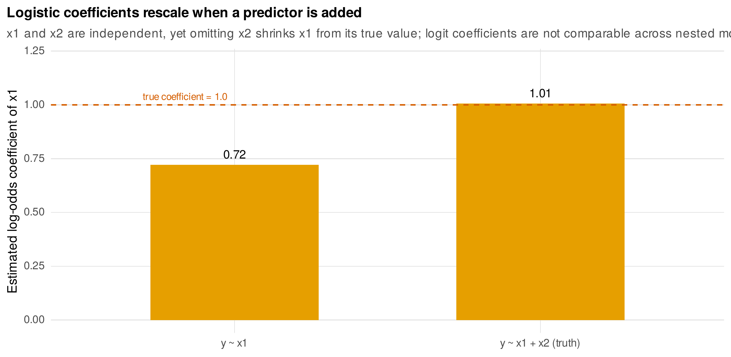
Note. A known-truth simulation with two independent predictors and a true first coefficient of \(1.0\). Regressing the binary outcome on the first predictor alone underestimates it at \(0.72\); adding the orthogonal second predictor returns the coefficient to its true value. Because the latent residual variance is fixed at \(\pi^2/3\), logistic coefficients are not comparable across nested models the way ordinary-regression coefficients are (Mood, 2010).
15.2 Estimation: Integrals Without Closed Forms
The likelihood of a GLMM requires integrating the random effects out of the joint density, and for a nonlinear link this integral has no closed form. Each cluster contributes a factor \(\int \prod_t f(y_{it}\mid \mathbf{u}_i)\,\phi(\mathbf{u}_i)\,d\mathbf{u}_i\), a product of non-normal densities weighted by the normal random-effect density, and no antiderivative exists. Estimation therefore rests on approximating the integral, and the approximation, not the model, is often what determines whether an analysis succeeds. Three methods span current practice. Penalized quasi-likelihood (PQL) linearizes the model around the current estimates and is fast, but it is badly biased for binary and low-count outcomes, understating both the fixed effects and the variance components, and it should be regarded as a legacy method rather than a default (Breslow & Clayton, 1993). The Laplace approximation replaces the integrand with a Gaussian matched at its mode and is the workhorse default of modern software, accurate enough for most designs. Adaptive Gauss-Hermite quadrature (AGQ) evaluates the integral at several points placed adaptively around the mode and converges to the exact likelihood as the number of points grows, at the cost of speed and a restriction, in common implementations, to a single scalar random effect. Table 15.2 summarizes the choices.
Table 15.2. Integral approximations for the generalized linear mixed model.
| Method | When adequate | Software |
|---|---|---|
| Penalized quasi-likelihood | Large counts, large clusters; avoid for binary | MASS::glmmPQL |
| Laplace | Most designs; the practical default | glmer, glmmTMB |
| Adaptive Gauss-Hermite | Binary or sparse outcomes, small clusters, large variances | glmer (nAGQ), GLMMadaptive |
| Bayesian (MCMC) | Complex random structures, separation, small samples | brms, MCMCglmm (Chapter 17) |
Note. The methods trade speed against accuracy. Penalized quasi-likelihood is fastest and least accurate; adaptive quadrature is most accurate for hard cases but restricted to a single scalar random effect in most implementations. When the design is difficult, a Bayesian fit (Chapter 17) is the robust fallback.
The choice matters most exactly where longitudinal psychology often operates: binary outcomes, few occasions, and substantial between-person variance. Figure 15.4 shows the divergence on the remission model, whose intercept variance is large. The Laplace approximation places the intercept at \(-5.22\) on the log-odds scale and the intercept standard deviation at \(2.68\), while fifteen-point adaptive quadrature moves them to \(-4.88\) and \(2.34\). The fixed effects of primary interest, the week slope and the treatment-by-week interaction, are more stable, but the intercept and the variance component shift enough to matter for any statement about baseline probability or between-person heterogeneity. The practical protocol is to fit with Laplace, then confirm the estimates with a few levels of adaptive quadrature when the outcome is binary and the variance appreciable; a material change is a signal to prefer the quadrature estimate and, in the hardest cases, to move to the Bayesian estimation of Chapter 17.
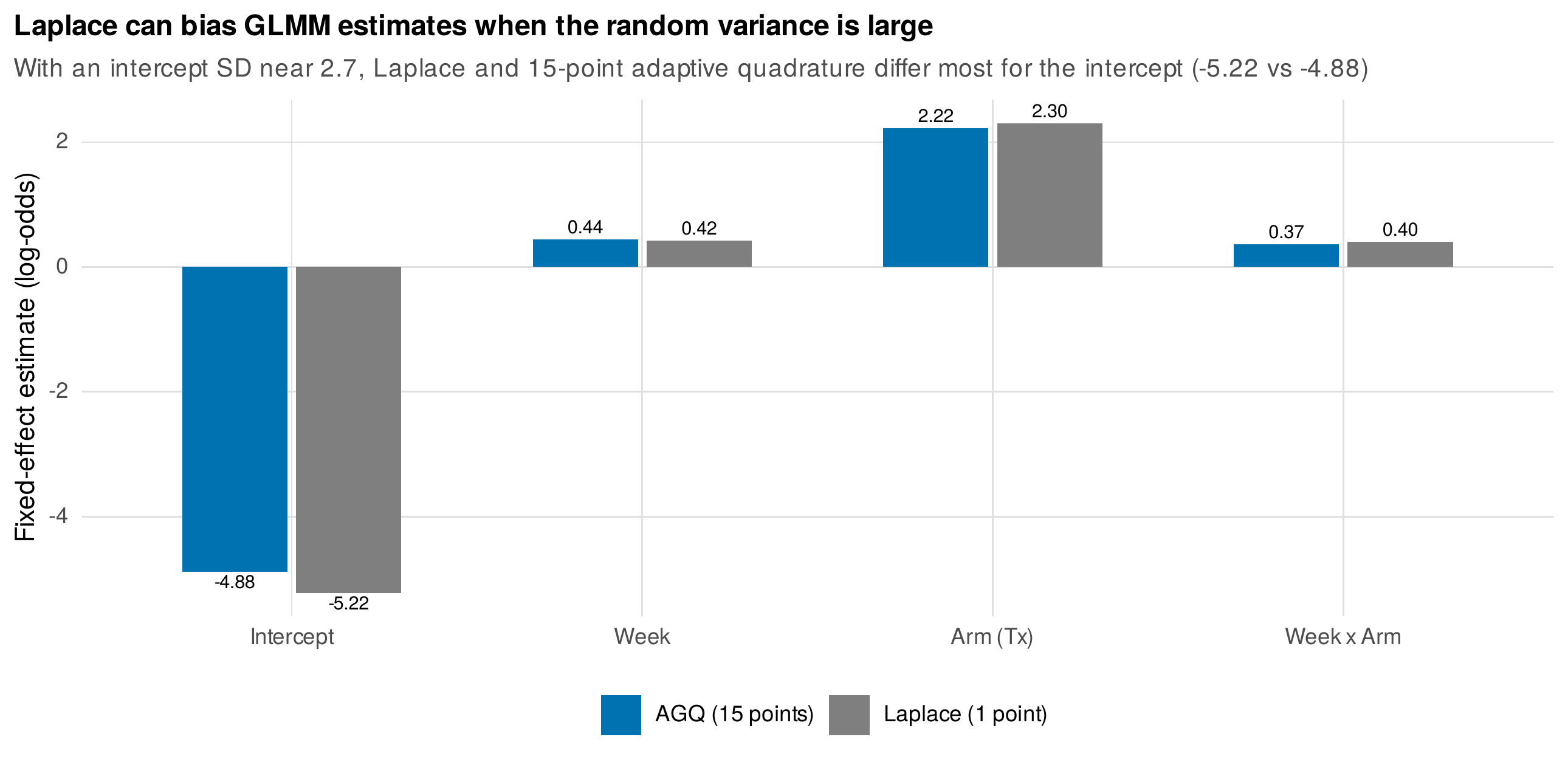
Note. Fixed-effect estimates of the binary remission model under the Laplace approximation (one quadrature point) and fifteen-point adaptive Gauss-Hermite quadrature. With an intercept standard deviation near \(2.7\) on the log-odds scale, the two methods differ most for the intercept, which the Laplace approximation places further from zero. The slope and interaction are more stable. Adaptive quadrature is the more accurate method for a binary outcome with large between-person variance.
Foundations Box • The attenuation factor and adaptive quadrature
The population-averaged and subject-specific logistic slopes are related, to a good approximation, by \(\bm{\gamma}_{\text{marginal}} \approx \bm{\gamma}_{\text{subject}} / \sqrt{1 + c^2\,\tau^2}\), with \(c = 16\sqrt{3}/(15\pi)\) and \(\tau^2\) the random-intercept variance, the same expression derived in Chapter 12. As \(\tau^2\) grows the marginal effect shrinks toward zero while the subject-specific effect is unchanged, which is why the two curves in Figure 15.2 diverge more for more heterogeneous outcomes. Adaptive Gauss-Hermite quadrature approximates the cluster likelihood as \(\int f(\mathbf{y}_i\mid u)\phi(u)\,du \approx \sum_{q=1}^{Q} w_q\, f(\mathbf{y}_i\mid a_q)\), evaluating the integrand at \(Q\) nodes \(a_q\) placed adaptively near the mode of the integrand rather than at fixed locations, so that a handful of well-placed nodes captures an integral that fixed-node quadrature would need many more to resolve. The Laplace approximation is the special case \(Q=1\).
15.3 Binary and Ordinal Outcomes
15.3.1 Binary Outcomes
The binary remission model is fitted by logistic growth in the log-odds, and its results are reported by walking from the coefficient scale to a scale readers can feel. With time centered at week eight, a point chosen because no patient has remitted at baseline and an intercept there would be unidentified, exactly the origin lesson of Chapter 14, the treatment-by-week interaction is \(0.40\) on the log-odds scale. Exponentiated, this is an odds ratio of about \(1.5\) per week for the treatment arm’s advantage in the growth of remission odds, but the odds ratio is a poor vehicle for communication, and the deliverable is the predicted probability trajectory. Figure 15.5 plots the model-implied remission probabilities for each arm over the study alongside the observed weekly rates, and it is this figure, not the coefficient table, that conveys the finding: remission is rare and similar in both arms through the first weeks, then rises steeply in the treatment arm to approach one half by week eleven while the control arm lags well behind. The between-person heterogeneity is summarized by the latent-scale intraclass correlation, computed as \(\tau_{00}/(\tau_{00}+\pi^2/3)\) because the level-one variance is the fixed \(\pi^2/3\); here it is \(.69\), indicating that most of the variation in the propensity to remit lies stably between patients.
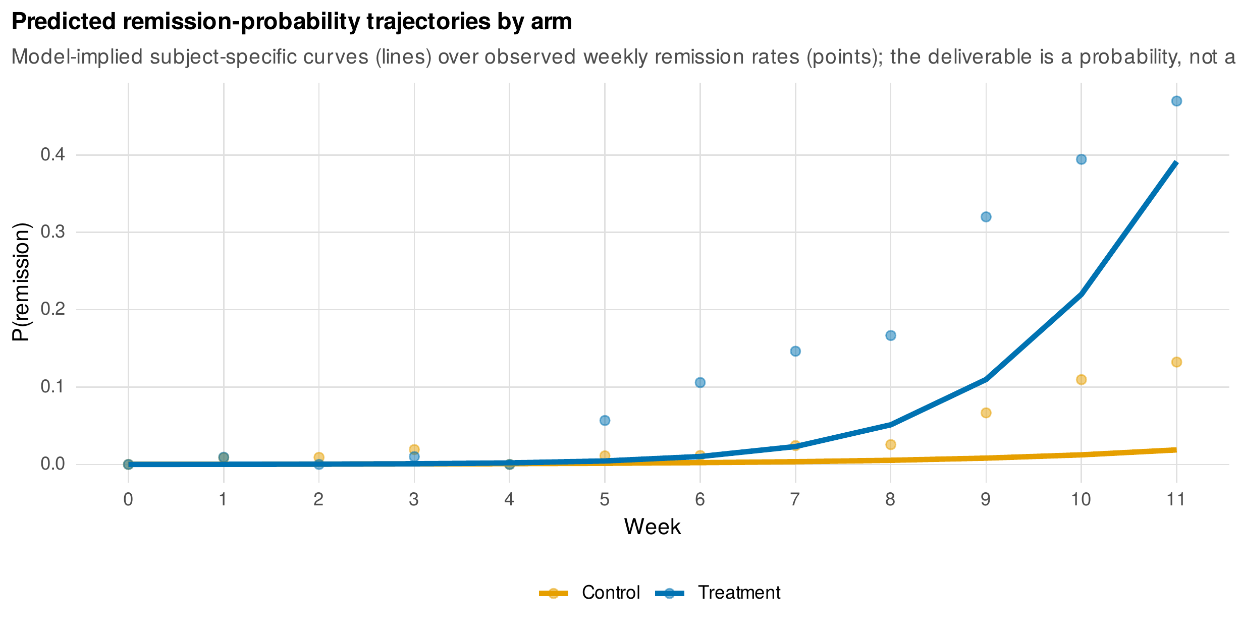
Note. Model-implied subject-specific remission probabilities by arm (lines) over the observed weekly remission rates (points). Remission is rare and comparable across arms early, then rises steeply in the treatment arm. A probability trajectory of this kind, not an odds ratio, is the deliverable of a binary longitudinal analysis.
15.3.2 Ordinal Outcomes
An ordinal outcome, such as a clinician’s four-level severity rating, is modeled by the cumulative-logit mixed model, which applies the logit link to the cumulative probabilities of being at or below each category. The model has one set of slopes and \(K-1\) thresholds, and its defining restriction is the proportional-odds assumption: a predictor shifts the odds of being in a higher category by the same amount at every threshold, so a single slope suffices for all category boundaries. On the severity data, fitted with a person random intercept, the week slope is \(-0.47\) on the cumulative-logit scale, meaning that each week multiplies the odds of being in a more severe category by about \(0.63\), and the treatment slope adds a further reduction. Figure 15.6 makes the fitted model legible by plotting the predicted category probabilities over time: mass drains out of the severe and moderate categories and accumulates in mild and remission as treatment proceeds. The proportional-odds assumption must be checked rather than assumed, by a test of whether separate slopes at each threshold improve the fit, and when it is violated the remedy is not to abandon the model but to relax it, allowing the offending predictor a partial or fully non-proportional effect, or to collapse sparse adjacent categories honestly. A nominal outcome without ordering would instead call for a multinomial mixed model, available through specialized packages, though the loss of the ordering usually costs power and interpretability when an order exists.
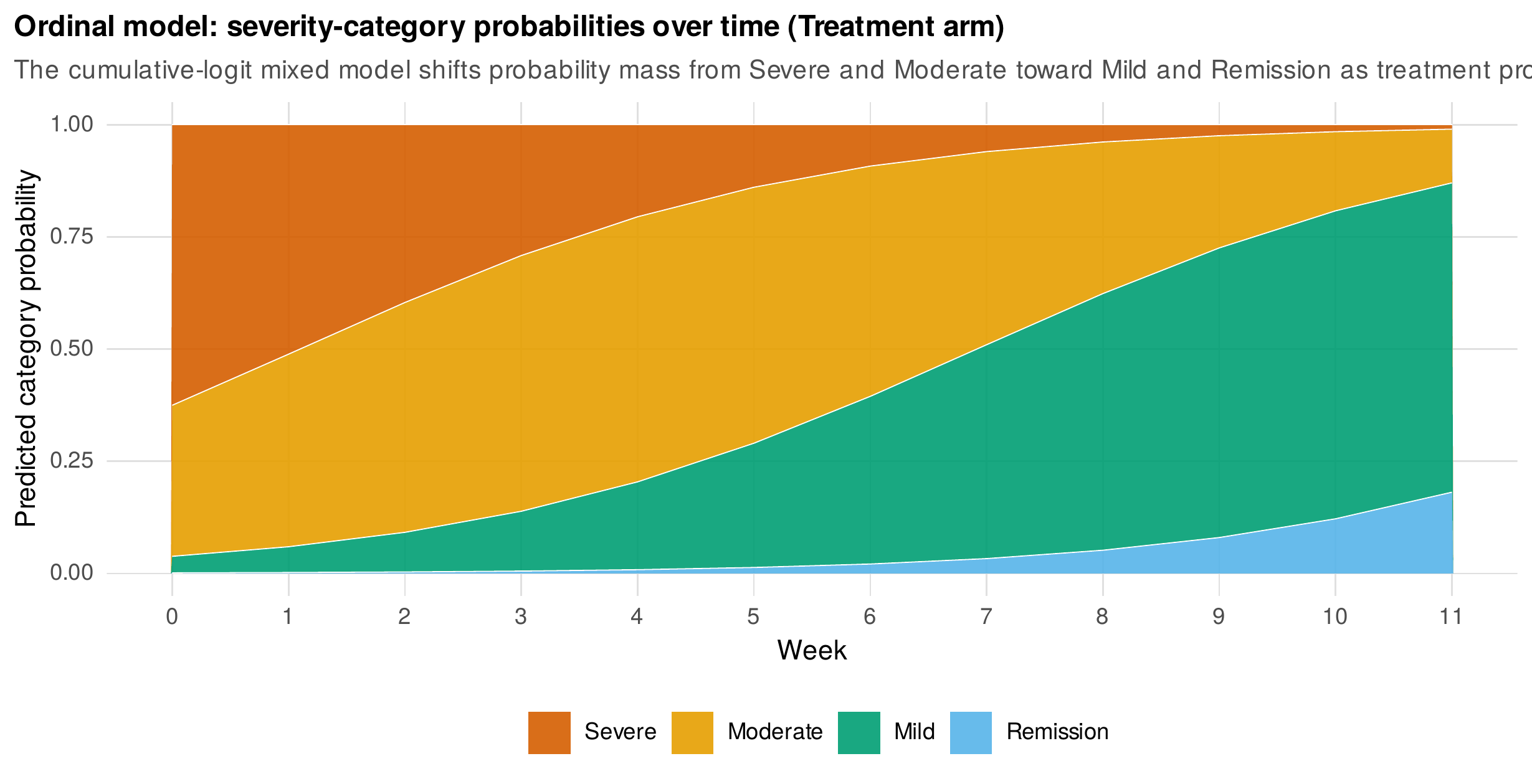
Note. Predicted probabilities of the four severity categories over weeks for the treatment arm, from the cumulative-logit mixed model. The stacked areas show probability mass shifting from severe and moderate toward mild and remission across the study. The model assumes proportional odds, that each predictor shifts the odds identically at every category boundary, an assumption that must be tested.
15.4 Count Outcomes
Counts, the daily tallies of behaviors that ambulatory studies collect, are modeled with a log link and a count distribution, and they raise two questions that continuous outcomes do not: whether the variance exceeds what the baseline distribution permits, and whether zeros occur more often than it predicts. The running example is a simulated daily-diary dataset of alcoholic drinks, ema_drinks, with a known data-generating process, measured over fourteen days with a varying number of waking hours per day.
The baseline model is the Poisson mixed model, \(\log \mathbb{E}(y_{it}) = \eta_{it} + \log(\text{exposure}_{it})\), in which the \(\log(\text{exposure})\) term is an offset, a predictor with its coefficient fixed at one, that converts the model from counts to rates and so accounts for unequal observation windows. Modeling drinks per waking hour rather than raw drinks matters whenever the window varies, as it does in real diaries where days differ in length and completeness. The Poisson makes a strong assumption, that the variance equals the mean, and it is usually wrong for behavioral counts. On the drinks data the Pearson dispersion is \(2.4\), more than twice the Poisson expectation of one, the signature of overdispersion. Two remedies are available and they encode different stories. The negative binomial adds a dispersion parameter that inflates the variance above the mean multiplicatively, appropriate when the extra variability is diffuse unexplained heterogeneity in the rate. An observation-level random effect, a separate random intercept for each observation, adds overdispersion through an explicit latent term, appropriate when the extra variability is thought of as occasion-specific perturbation. Both cure the immediate symptom; the choice is a modeling judgment about the source of the excess variance.
Excess zeros are a distinct problem from overdispersion, and the more interesting one, because the zeros carry substantive meaning. Figure 15.7 shows the observed distribution of daily drinks against the fitted Poisson and negative-binomial probabilities. The Poisson fails twice over, predicting far too few zeros, \(35\) percent against the observed \(52\), and too little mass in the tail. The negative binomial, by fattening the whole distribution, matches the observed zero fraction well, at \(51\) percent, which illustrates that overdispersion and excess zeros are entangled: a distribution with heavier dispersion also carries more zeros. But matching the zero count is not the same as modeling the zero process, and two models make the process explicit in different ways. Figure 15.8 draws the distinction as a pair of process trees.
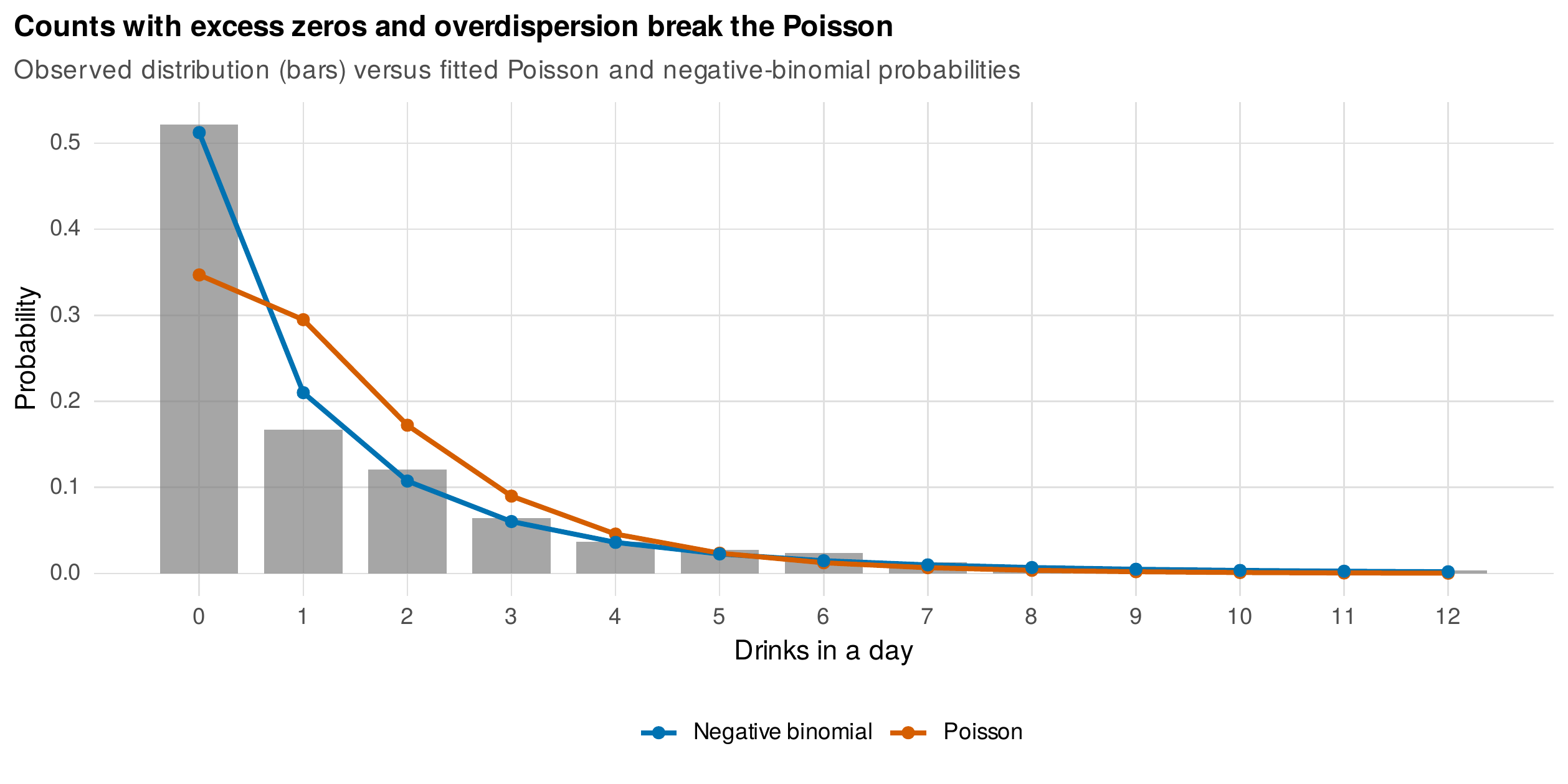
Note. The observed distribution of daily drinks (bars) with the fitted marginal probabilities of the Poisson and negative-binomial mixed models. The Poisson predicts too few zero days (\(35\) percent against \(52\) observed) and too thin a tail; the negative binomial, by adding dispersion, matches the zero fraction and the tail far better. Overdispersion and excess zeros are entangled symptoms.
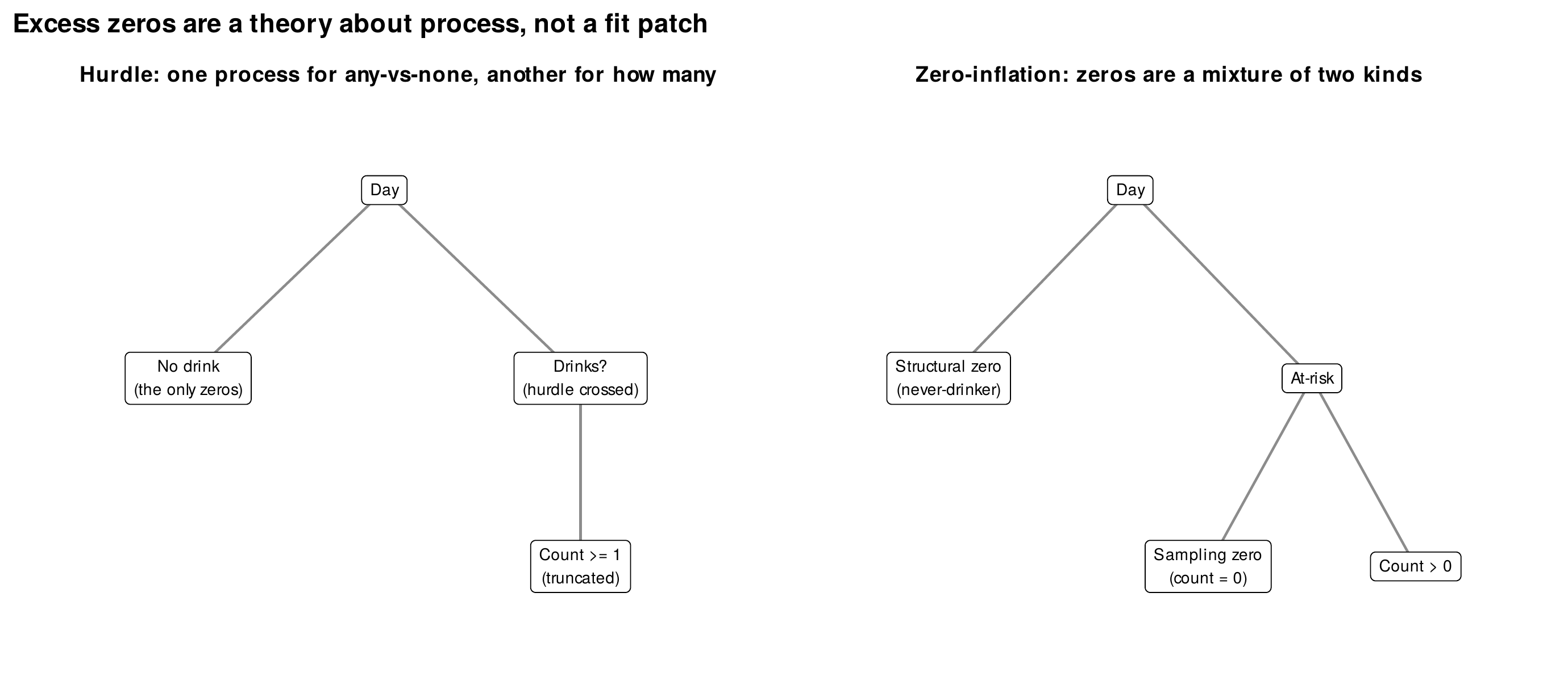
Note. Two accounts of excess zeros. The hurdle model (left) posits one process that decides any-versus-none and a second, truncated, process for the amount among those who cross the hurdle, so every zero is a structural zero. The zero-inflation model (right) posits a mixture in which some units are structural zeros, never at risk, while the rest follow a count distribution that can itself yield sampling zeros. The choice between them is a substantive claim about how the zeros arise.
The hurdle model is a two-part model: one process, a logistic model, decides whether the count clears a hurdle at zero, and a second process, a zero-truncated count model, governs the amount among those that clear it. Every zero is of one kind, a failure to clear the hurdle, and the two parts answer two research questions, whether a behavior occurred at all and, given that it occurred, how much. The zero-inflation model tells a different story, a mixture of two latent kinds of unit: structural zeros that are never at risk, drawn with some probability, and the remainder that follow an ordinary count distribution which can itself produce sampling zeros. The distinction is substantive, not statistical. Abstainers who never drink are structural zeros suited to a mixture; a person who drinks but had none on a particular day is a sampling zero. Whether a population contains genuine never-drinkers or only occasional non-drinking days is a theory of the phenomenon, and it, not an information criterion, should select the model (Atkins & Gallop, 2007; Atkins et al., 2013). On the drinks data the hurdle’s two parts recover their generating values well, a weekend log-odds of \(1.2\) for drinking at all against a true \(1.1\), and the fitted hurdle reproduces the observed zero fraction almost exactly. Table 15.3 organizes the diagnosis and the remedies.
Table 15.3. Diagnosing and modeling overdispersion and excess zeros.
| Symptom | Candidate model | Substantive meaning |
|---|---|---|
| Variance exceeds the mean | Negative binomial | Diffuse unexplained heterogeneity in the rate |
| Variance exceeds the mean | Observation-level random effect | Occasion-specific perturbations of the rate |
| More zeros than the count model allows | Hurdle (two-part) | One process for any-versus-none, another for the amount |
| More zeros, and a subpopulation is never at risk | Zero-inflation (mixture) | Structural zeros from never-at-risk units plus sampling zeros |
Note. Overdispersion and excess zeros are related but distinct. The choice between a hurdle and a zero-inflation model is a claim about how the zeros arise, abstainers versus non-drinking days, and should be made on theory, then checked by fit, not selected by fit alone.
15.5 Validation and Reporting
A fitted GLMM must be checked, and the ordinary residual plots of linear models are uninformative for discrete outcomes, because a residual from a binary or low-count observation is not even approximately normal. The modern standard is the simulation-based residual: for each observation the fitted model is used to simulate many replicate outcomes, and the residual is the position of the observed value within its own simulated distribution, a quantity that is uniform on the unit interval when the model is correct regardless of the outcome’s distribution (Hartig’s DHARMa implements this; the same quantity is computed transparently from any fitted model’s simulate method). Figure 15.9 applies it to the count models. The Poisson’s scaled residuals depart markedly from the uniform diagonal, with a maximum deviation of \(0.26\), the fingerprint of its misfit, while the negative binomial’s residuals track the diagonal much more closely. Such plots also carry dedicated tests for overdispersion, for excess zeros, and for residual structure within clusters, and they are the recommended first diagnostic for any GLMM.
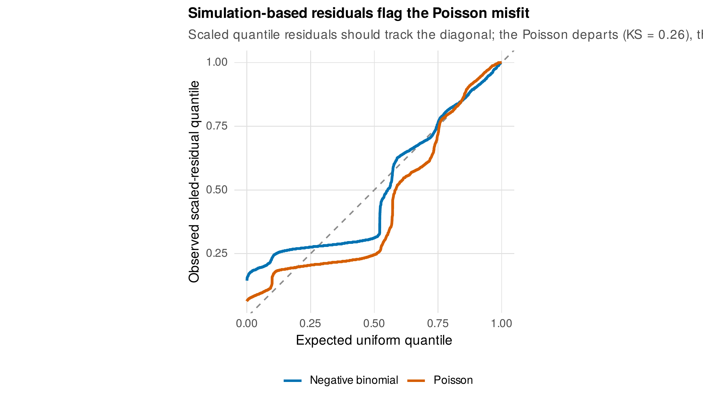
Note. Simulation-based scaled quantile residuals for the Poisson and negative-binomial count models, plotted against their expected uniform quantiles. Under a correct model the residuals track the diagonal. The Poisson departs (maximum deviation \(0.26\)), reflecting its unmodeled overdispersion and excess zeros; the negative binomial is closer. This diagnostic works for any discrete outcome, where ordinary residual plots do not.
Reporting a GLMM well is largely a matter of interpretation discipline, and the recurring failure is to report bare coefficients or odds ratios that few readers can translate into consequences. Table 15.4 sets out the elements. The family and link must be named and justified, the estimation method and its settings stated, including the number of quadrature points when adaptive quadrature is used, and the interpretation scale kept explicit at every turn, since a coefficient is subject-specific and an odds ratio is not a risk ratio. Above all, the results should be carried to predicted probabilities, rates, or category probabilities, displayed as trajectories or profiles, because those are the quantities a reader can evaluate. Table 15.5 lays out the interpretation pipeline from the coefficient scale to the reportable quantity.
Table 15.4. A reporting checklist for a generalized linear mixed model.
| Element | What to report |
|---|---|
| Family and link | The outcome distribution and link function, with justification |
| Estimation | The approximation method and its settings, including the quadrature points for adaptive quadrature |
| Interpretation scale | Coefficients named as subject-specific; odds ratios distinguished from risk ratios |
| Predicted quantities | Probabilities, rates, or category profiles, displayed as trajectories |
| Random effects | The variance components and the latent-scale intraclass correlation |
| Dispersion and zeros | For counts, the dispersion treatment and the zero model with its rationale |
| Diagnostics | Simulation-based residual checks |
Note. The elements a generalized-linear-mixed-model write-up must include beyond a linear-model report, extending the checklist of Chapter 13. The recurring failure is to stop at the coefficient scale; every result should reach an interpretable predicted quantity.
Table 15.5. The interpretation pipeline for a generalized linear mixed model.
| Outcome | Coefficient scale | Reportable quantity |
|---|---|---|
| Binary | Log-odds (subject-specific) | Predicted probability trajectory; odds ratio with the conditional caveat |
| Ordinal | Cumulative log-odds | Category-probability profiles over time |
| Count | Log-rate | Predicted rate per exposure unit; incidence-rate ratio |
| Any | Fixed-effect coefficient | Average marginal effect over the random-effect and covariate distributions |
Note. The coefficient is where estimation ends, not where reporting ends. Each outcome type has a natural interpretable quantity that translates the model onto a scale readers can evaluate, obtained by mapping predictions through the inverse link and, for population-averaged quantities, averaging over the random effects.
15.6 Running the Generalized Linear Mixed Model in R
The binary and count models are fitted with glmer from lme4, the ordinal model with clmm from ordinal, and the count extensions with glmer.nb or the more flexible glmmTMB. Adaptive quadrature is requested through the nAGQ argument for a scalar random effect.
library(lme4); library(ordinal)
rct <- transform(rct, week_c = week - 8,               # origin at an estimable point
                 remit = as.integer(hdrs <= 7))

# --- Binary: logistic growth, Laplace then adaptive quadrature ---
mB  <- glmer(remit ~ week_c*arm + (1 | patient_id), data = rct,
             family = binomial, nAGQ = 1)              # Laplace
mB2 <- update(mB, nAGQ = 15)                           # 15-point AGQ
tau <- VarCorr(mB)$patient_id[1]; tau/(tau + pi^2/3)   # latent-scale ICC

# --- Ordinal: cumulative-logit mixed model with proportional odds ---
mO <- clmm(severity ~ week + arm + (1 | patient_id), data = rct)
Counts use a log-exposure offset; overdispersion is treated with the negative binomial, and the hurdle is fitted as two parts or in a single call with glmmTMB.
# --- Count: Poisson with offset, then negative binomial ---
mP  <- glmer(drinks ~ weekend + (1|person), offset = log(awake_hours/16),
             data = ema, family = poisson)
mNB <- glmer.nb(drinks ~ weekend + (1|person) + offset(log(awake_hours/16)), data = ema)

# --- Hurdle in one call (glmmTMB): amount model + zero-hurdle model ---
# glmmTMB(drinks ~ weekend + (1|person), ziformula = ~., family = truncated_nbinom2, data = ema)

# --- Simulation-based residuals for any fitted model ---
# DHARMa::simulateResiduals(mNB) |> plot()
The complete analysis, including the Laplace-versus-quadrature comparison, the conditional-versus-marginal computation, the coefficient-rescaling demonstration, and the count-model gallery with simulation-based residuals, is the shipped script ch15_analysis_V01.R, with figures drawn by ch15_figures_V01.R and the count dataset generated by gen_ema_drinks_V01.R. The glmmTMB package fits zero-inflation and hurdle models in a single call and is the recommended tool for count outcomes; GLMMadaptive provides adaptive quadrature for models with a random slope; and DHARMa automates the simulation-based diagnostics.
Software Note • glmer, glmmTMB, and the categorical tradition
For binary and ordinal outcomes glmer and clmm suffice, while for counts, and especially for overdispersion and excess zeros, glmmTMB is more capable, fitting negative-binomial, zero-inflated, and hurdle models with random effects in one call through its family and ziformula arguments; GLMMadaptive adds adaptive quadrature when a random slope rules out glmer’s nAGQ. Across programs the same model appears under different names: SAS fits it with PROC GLIMMIX, Stata with meglm and its family-specific commands, and SPSS with GENLINMIXED. The structural-equation tradition, taken up in Chapter 18, fits categorical outcomes through a probit link with weighted least squares (the WLSMV estimator in Mplus and lavaan), which estimates the thresholds of Figure 15.1 directly and connects to item response theory; the likelihood-based logit models of this chapter and the limited-information probit models of that one answer the same substantive questions by different estimation routes.
15.7 Common Misconceptions
Several beliefs about generalized linear mixed models mislead. The first is that logistic coefficients compare across models as linear coefficients do; because the latent residual variance is fixed, adding any predictor rescales the others, so cross-model comparison of coefficients is invalid and predicted probabilities or average marginal effects must be compared instead (Figure 15.3). The second is that a GLMM coefficient and a marginal-model coefficient estimate the same thing; the GLMM coefficient is subject-specific and the generalized estimating equation coefficient is population-averaged, and the two differ by the attenuation of Chapter 12. The third is that overdispersion is a defect of the Poisson to be patched by the negative binomial; it is often substantive, and an observation-level random effect or a mixture may better represent its source. The fourth is that zero-inflation is a matter of fit; the choice between a hurdle and a mixture is a theory of how the zeros arise and should be argued, not selected by an information criterion. The fifth is that a violated proportional-odds assumption invalidates the ordinal model; a partial or non-proportional relaxation preserves the model while freeing the offending predictor.
Common Pitfall • five errors in GLMM practice
First, reporting bare odds ratios as if they were risk ratios: an odds ratio overstates a risk ratio when the outcome is common, and neither is a probability; carry results to predicted probabilities. Second, comparing logit coefficients across nested models: the fixed residual variance rescales them, so a coefficient that changes when a covariate is added is not evidence of mediation. Third, trusting Laplace for a binary outcome with large between-person variance: confirm with adaptive quadrature, which can move the estimates materially (Figure 15.4). Fourth, assuming a Poisson without checking dispersion: a Pearson dispersion far above one signals overdispersion, and simulation-based residuals will reveal it. Fifth, choosing zero-inflation over a hurdle by AIC alone: decide by whether structural, never-at-risk zeros are substantively real.
In Practice • separation in binary and sparse GLMMs
Binary longitudinal outcomes are prone to separation, in which a level of a predictor perfectly predicts the outcome, sending a coefficient or an intercept toward infinity and the fit into non-convergence. It arises naturally when an event is impossible early, as remission is at baseline, and it appears as an enormous coefficient with an enormous standard error, or as an outright estimation failure. The remedies are, in order, to recenter time or rescale predictors so the intercept lands in an estimable region, exactly the origin decision of Chapter 14; to collapse or exclude structurally empty cells honestly; and, when separation is intrinsic to the data, to add weak-information regularization through a penalized likelihood or a Bayesian prior (Chapter 17), which keeps the estimate finite. In this chapter’s remission model the time origin was moved from baseline, where no patient had remitted, to week eight, where the intercept is identified.
Chapter Summary
The generalized linear mixed model extends the linear mixed model to binary, ordinal, and count outcomes by inserting a link function, keeping the random effects intact. For binary and ordinal outcomes it is equivalently a threshold model on a latent variable whose residual variance is fixed by the link (Figure 15.1), a fact with two consequences: coefficients are subject-specific and differ from the population-averaged effects of Chapter 12 by an attenuation that grows with the random variance (Figure 15.2), and logistic coefficients do not compare across models because the fixed residual variance rescales them (Figure 15.3). The likelihood requires an integral approximation, and the choice among penalized quasi-likelihood, Laplace, and adaptive quadrature matters most for binary outcomes with small clusters and large variances, where Laplace can bias the intercept and the variance component (Figure 15.4). Binary outcomes are reported as predicted probability trajectories (Figure 15.5) and summarized by a latent-scale intraclass correlation; ordinal outcomes by a cumulative-logit model with a checkable proportional-odds assumption and category-probability profiles (Figure 15.6). Counts use a log link with an exposure offset, and they raise overdispersion, cured by the negative binomial or an observation-level random effect, and excess zeros, modeled by a hurdle or a zero-inflation mixture whose difference is a theory of the zeros, not a fit statistic (Figures 15.7 and 15.8). Simulation-based residuals are the diagnostic standard for discrete outcomes (Figure 15.9), and reporting carries every result to an interpretable predicted quantity.
Where to Go Next
The generalized linear mixed model is the subject-specific counterpart to the marginal model of Chapter 12, and the two chapters should be read as a pair on the interpretation of nonlinear-link longitudinal models. Chapter 16 turns to modeling the within-person variance itself, the mixed-effects location-scale model, which treats variability as an outcome rather than a nuisance. Chapter 17 supplies the Bayesian estimation that rescues the separation-prone and weakly identified models this chapter’s harder cases produce, and that fits the complex random structures adaptive quadrature cannot. Chapter 18 approaches categorical outcomes from the measurement side, where the thresholds of the latent-variable formulation become the item parameters of a categorical measurement model estimated by weighted least squares. Chapter 23 deploys binary and count outcomes on intensive diary data, and Chapter 29 reveals discrete-time survival analysis to be a binary generalized linear mixed model in disguise, the hazard of an event at each occasion modeled exactly as remission was here.
Exercises
- 15.1 Laplace versus quadrature. Simulate binary mixed-model data at a small and a large random-intercept variance, fit each with Laplace and with high-order adaptive quadrature, and tabulate the bias in the fixed effects and the variance component against the known truth.
- 15.2 From coefficients to probabilities. On a binary longitudinal outcome, fit the logistic growth model, convert the coefficients to an odds ratio and then to a predicted probability trajectory, and write the results paragraph so that no bare odds ratio stands without an accompanying probability.
- 15.3 Proportional odds. Fit a cumulative-logit mixed model to an ordinal outcome with a planted proportional-odds violation, detect it by comparing proportional and partial-proportional specifications, and report the estimand-appropriate remedy.
- 15.4 Counts to hurdle. On a count diary outcome, fit the Poisson with an exposure offset, diagnose overdispersion, move to the negative binomial, then to a hurdle, and defend the hurdle over a zero-inflation mixture in a short paragraph grounded in the process, not the fit.
- 15.5 Residual forensics. Given four fitted models with distinct planted misspecifications, an unmodeled overdispersion, an unmodeled excess of zeros, a missing nonlinearity, and a correct model, identify each from its simulation-based residual panel.
References
Agresti, A. (2013). Categorical data analysis (3rd ed.). Wiley.
Atkins, D. C., Baldwin, S. A., Zheng, C., Gallop, R. J., & Neighbors, C. (2013). A tutorial on count regression and zero-altered count models for longitudinal substance use data. Psychology of Addictive Behaviors, 27(1), 166–177. https://doi.org/10.1037/a0029508
Atkins, D. C., & Gallop, R. J. (2007). Rethinking how family researchers model infrequent outcomes: A tutorial on count regression and zero-inflated models. Journal of Family Psychology, 21(4), 726–735. https://doi.org/10.1037/0893-3200.21.4.726
Bolker, B. M., Brooks, M. E., Clark, C. J., Geange, S. W., Poulsen, J. R., Stevens, M. H. H., & White, J.-S. S. (2009). Generalized linear mixed models: A practical guide for ecology and evolution. Trends in Ecology & Evolution, 24(3), 127–135. https://doi.org/10.1016/j.tree.2008.10.008
Breslow, N. E., & Clayton, D. G. (1993). Approximate inference in generalized linear mixed models. Journal of the American Statistical Association, 88(421), 9–25. https://doi.org/10.1080/01621459.1993.10594284
Brooks, M. E., Kristensen, K., van Benthem, K. J., Magnusson, A., Berg, C. W., Nielsen, A., Skaug, H. J., Mächler, M., & Bolker, B. M. (2017). glmmTMB balances speed and flexibility among packages for zero-inflated generalized linear mixed modeling. The R Journal, 9(2), 378–400. https://doi.org/10.32614/RJ-2017-066
Bürkner, P.-C. (2017). brms: An R package for Bayesian multilevel models using Stan. Journal of Statistical Software, 80(1), 1–28. https://doi.org/10.18637/jss.v080.i01
Christensen, R. H. B. (2019). ordinal: Regression models for ordinal data (R package version 2019.12-10) [Computer software]. https://CRAN.R-project.org/package=ordinal
Hedeker, D., & Gibbons, R. D. (1994). A random-effects ordinal regression model for multilevel analysis. Biometrics, 50(4), 933–944. https://doi.org/10.2307/2533433
Hedeker, D., & Gibbons, R. D. (2006). Longitudinal data analysis. Wiley. https://doi.org/10.1002/0470036486
Lambert, D. (1992). Zero-inflated Poisson regression, with an application to defects in manufacturing. Technometrics, 34(1), 1–14. https://doi.org/10.2307/1269547
Mood, C. (2010). Logistic regression: Why we cannot do what we think we can do, and what we can do about it. European Sociological Review, 26(1), 67–82. https://doi.org/10.1093/esr/jcp006
Mullahy, J. (1986). Specification and testing of some modified count data models. Journal of Econometrics, 33(3), 341–365. https://doi.org/10.1016/0304-4076(86)90002-3
Nakagawa, S., & Schielzeth, H. (2013). A general and simple method for obtaining \(R^2\) from generalized linear mixed-effects models. Methods in Ecology and Evolution, 4(2), 133–142. https://doi.org/10.1111/j.2041-210x.2012.00261.x
Zeger, S. L., Liang, K.-Y., & Albert, P. S. (1988). Models for longitudinal data: A generalized estimating equation approach. Biometrics, 44(4), 1049–1060. https://doi.org/10.2307/2531734