Chapter 16
Modeling Within-Person Variability: Mixed-Effects Location-Scale Models
Every model to this point has treated variability as noise. The residual variance was a nuisance to be estimated and divided out, an obstacle between the data and the mean structure that was the real object of study. This chapter inverts that stance and makes the variance the dependent variable. For a large class of psychological questions the within-person variability is not error but the phenomenon: affective instability in borderline and bipolar conditions, the inconsistency of cognitive performance that marks aging, the irregularity of a sleep schedule, the volatility of a symptom that a therapy is meant to calm. In each the scientific quantity is how much a person swings, not where the person sits on average, and two people with identical means can have entirely different prognoses because one is stable and the other labile. Chapter 7 introduced indices of intraindividual variability and catalogued their flaws; this chapter supplies the model-based repair. The mixed-effects location-scale model places a submodel on the mean and a second submodel on the within-person variance, lets both carry random effects, and estimates the correlation between a person’s level and a person’s volatility. It is the clearest payoff in the book of the index-now-model-later logic, and it is the first chapter where Bayesian estimation becomes the natural engine, a handoff that Chapter 17 completes.
Learning Objectives
After working through this chapter, you should be able to: (1) explain why within-person variance is a substantive quantity and why two-stage standard-deviation indices are deficient as estimates and as predictors; (2) specify the mixed-effects location-scale model, with a location submodel, a log-linear scale submodel carrying a random scale effect, and a correlation between the location and scale random effects; (3) interpret scale-model coefficients on the multiplicative variance scale; (4) fit the model, read its output, and recover its parameters; (5) test predictors of variability with proper uncertainty; (6) situate the model among its distributional relatives; and (7) validate it with variance-targeted posterior predictive checks and report it to publication standard.
16.1 Variability as Signal
The premise of the chapter is a gallery of people who are identical in the mean and different in everything that matters. Figure 16.1 shows four persons with the same average negative affect and sharply different within-person variability, from nearly flat to wildly swinging. In a clinical setting these are four different patients: the stable one and the highly labile one may share a diagnosis and a mean symptom level yet face different risks, respond to different treatments, and warrant different monitoring. The tradition of studying such differences runs through the work on affective instability in psychopathology (Ebner-Priemer et al., 2009; Jahng et al., 2008), the study of performance inconsistency as an early marker of cognitive decline (Hultsch et al., 2002), and the broader program of treating short-term intraindividual variability as a stable individual-differences construct (Wang et al., 2012). In every case the claim is the same: the variance is the phenomenon, and a method that models only the mean discards it.
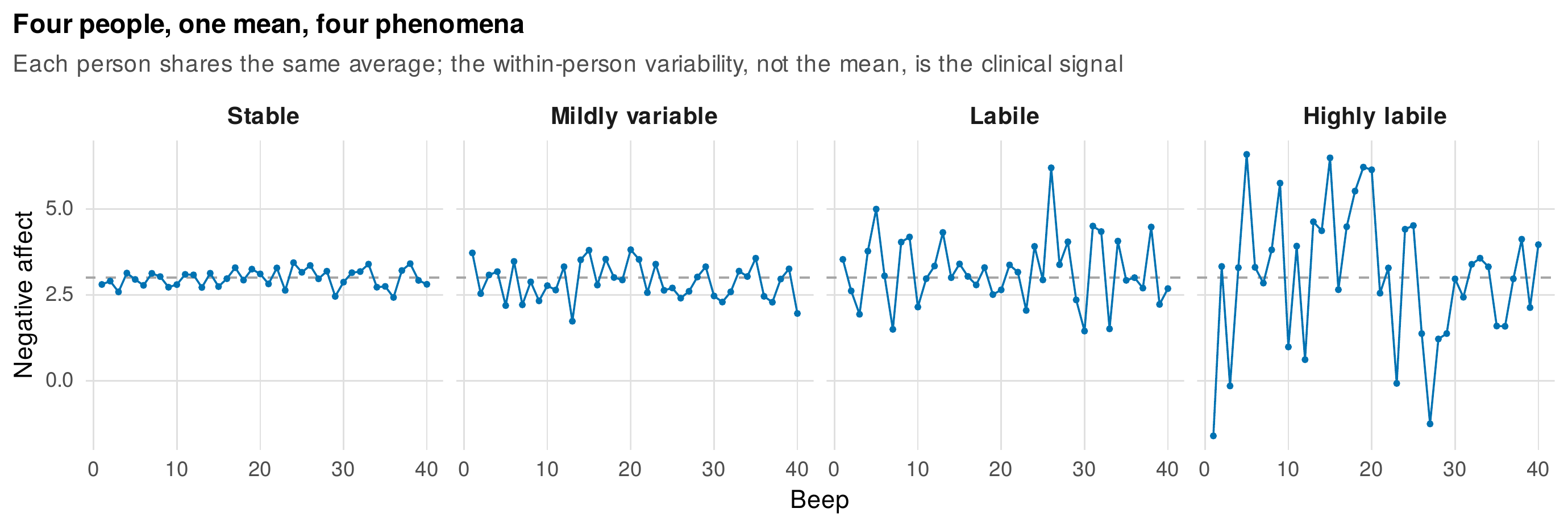
Note. Four simulated persons with the same average negative affect and increasing within-person variability, from stable to highly labile. The mean cannot distinguish them; the within-person standard deviation can, and it is frequently the quantity of clinical interest. This figure extends the intraindividual-variability display of Chapter 7 with an explicit substantive reading.
Chapter 7 measured this variability with the intraindividual standard deviation, computed one person at a time, and warned that the index is fragile. The warning can now be made precise as a four-part deficiency audit. First, the two-stage standard deviation is estimated with error that depends on the number of occasions, so a person measured on twenty beeps has a far noisier estimate than one measured on fifty, and Figure 16.2 shows the resulting scatter. Second, there is no shrinkage: each person’s estimate stands alone, so the extreme values, which fall disproportionately on the persons with the fewest occasions, are taken at face value rather than pulled toward the group. Third, the index confounds level with variability whenever the two are related, and the right panel of Figure 16.2 shows exactly the positive coupling between mean and standard deviation that a bounded or floor-prone scale induces, so that a difference in variability may be an artifact of a difference in level. Fourth, when the index is then carried into a second analysis as a predictor, its estimation error becomes error-in-variables that biases the downstream coefficient, an instance of the plug-in fallacy that recurs whenever a noisy estimate is treated as a known quantity. A model-based approach must repair all four: it must borrow strength across persons, admit covariates at both levels, model level and variability jointly, and propagate the uncertainty in the person-specific variability into whatever uses it. Table 16.1 sets the two approaches side by side.
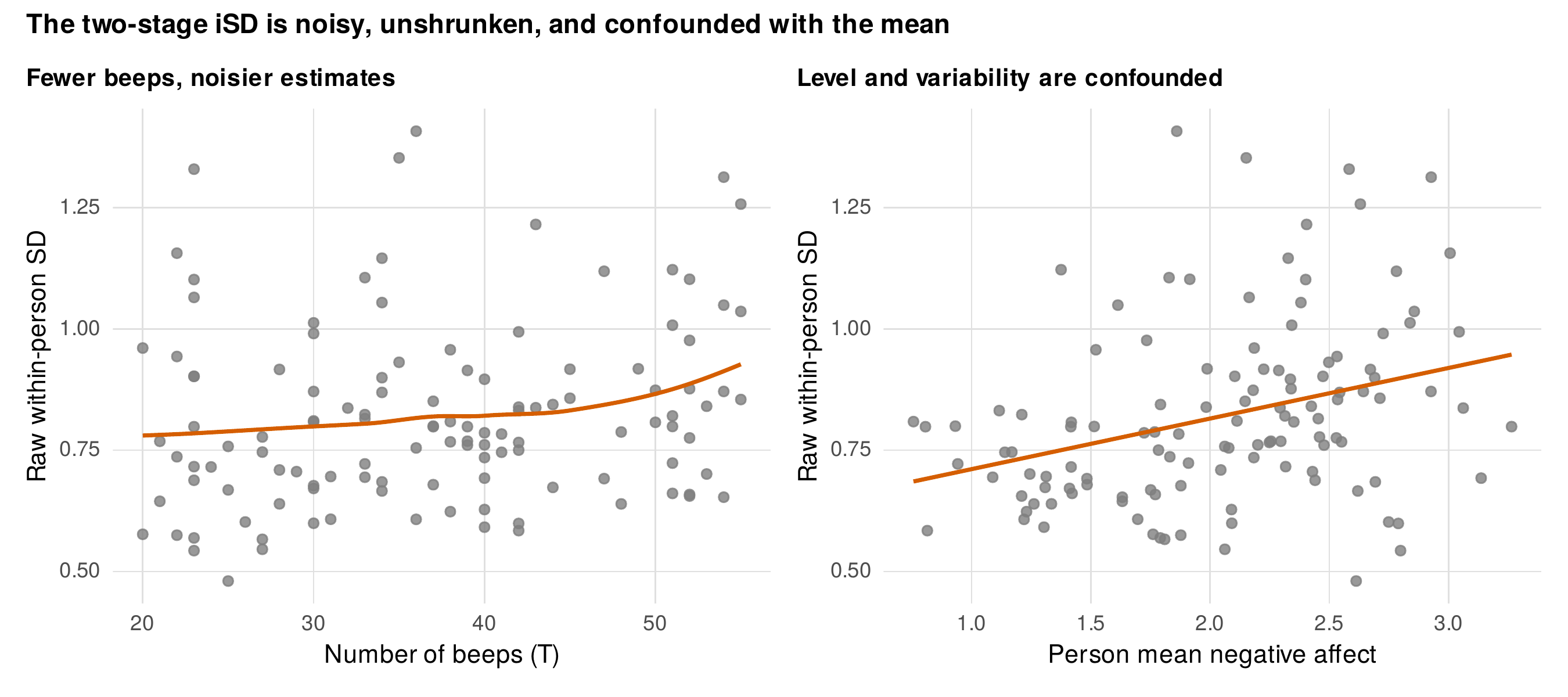
Note. Left: the raw within-person standard deviation against the number of beeps, showing that fewer occasions give noisier and more extreme estimates with no shrinkage. Right: the raw within-person standard deviation against the person mean, showing that level and variability are confounded when the outcome has a floor. Both deficiencies are repaired by a model that estimates person volatility with shrinkage and separates it from the mean.
Table 16.1. Two-stage indices versus a model-based location-scale approach.
| Capability | Two-stage iSD | Location-scale model |
|---|---|---|
| Borrows strength across persons (shrinkage) | No | Yes |
| Handles unequal numbers of occasions | Poorly | Yes |
| Covariates for variability (who, when) | No | Yes |
| Models level and variability jointly | No | Yes |
| Propagates uncertainty downstream | No | Yes |
Note. The two-stage intraindividual standard deviation computes a separate variability estimate per person and carries it forward as if known. The mixed-effects location-scale model estimates the same quantity with shrinkage, admits predictors of variability at both levels, and preserves its uncertainty.
16.2 The Model, Built in Three Steps
The mixed-effects location-scale model is best assembled in three steps, each a recognizable extension of the last. The first step is heterogeneous level-one variance. The ordinary mixed model assumes a single residual variance \(\sigma^2\) for everyone; the first relaxation lets that variance differ by group or by a covariate, the familiar territory of the residual-variance functions of Chapter 14. The second step makes the variance a regression. Rather than a separate variance per group, a log-linear scale submodel writes the log of the within-person variance as a linear function of predictors, \(\log \sigma^2_{it} = \alpha_0 + \alpha_1 x_{it}\), so that a covariate can raise or lower momentary variability. The log link is not incidental: it keeps the variance positive for any values of the coefficients, and it gives the coefficients a multiplicative reading, because a one-unit change in the predictor multiplies the variance by \(e^{\alpha_1}\). The third step adds a random effect to the scale submodel. Persons differ in their residual volatility beyond what the covariates explain, and a random scale effect \(\omega_i\) captures that difference, \(\log \sigma^2_{it} = \alpha_0 + \alpha_1 x_{it} + \omega_i\), so that each person has a personal baseline volatility just as the location submodel gives each person a personal baseline level.
The full model couples the two submodels and, crucially, allows their random effects to correlate. The location submodel is \(y_{it} = \gamma_{0} + \gamma_{1} x_{it} + u_{i} + \varepsilon_{it}\) with \(\varepsilon_{it} \sim N(0, \sigma^2_{it})\), the scale submodel is \(\log \sigma^2_{it} = \alpha_0 + \alpha_1 x_{it} + \omega_i\), and the two person effects are drawn together, \((u_i, \omega_i)' \sim N(\mathbf{0}, \mathbf{\Sigma})\), with a correlation \(\rho\) between them. Figure 16.3 draws the architecture. The correlation \(\rho\) is the parameter with the substantive punch: it asks whether people who are higher on average are also more variable, whether, for instance, patients with higher mean negative affect are also more volatile in it, a question that no two-stage analysis can pose because it never estimates the two quantities in a common model. Table 16.2 is a glossary of the parameters and how each is read.
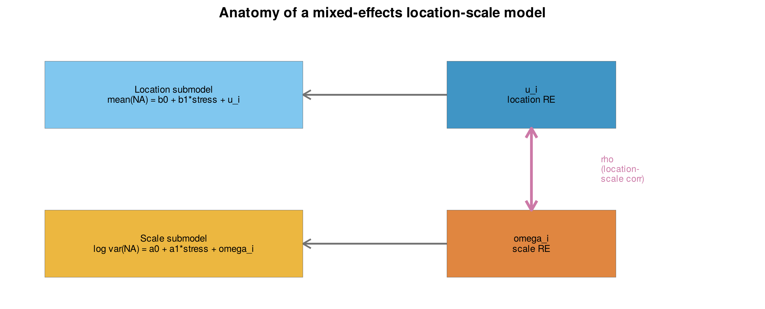
Note. The location submodel places a person random intercept \(u_i\) on the mean; the scale submodel places a person random intercept \(\omega_i\) on the log within-person variance; a within-person predictor can enter either submodel. The two random effects are drawn from a joint distribution with a correlation \(\rho\), the location-scale correlation that links a person’s level to a person’s volatility.
Table 16.2. A glossary of the location-scale model parameters.
| Symbol | Submodel | Interpretation |
|---|---|---|
| \(\gamma_1\) | Location | Effect of the predictor on the mean level |
| \(\alpha_1\) | Scale | Effect of the predictor on the log within-person variance; the variance is multiplied by \(e^{\alpha_1}\) per unit |
| \(u_i\) | Location (random) | Person departure in mean level; variance \(\tau_u^2\) |
| \(\omega_i\) | Scale (random) | Person departure in log volatility; variance \(\tau_\omega^2\) |
| \(\rho\) | Both | Correlation of level and volatility across persons |
Note. The location parameters are read as in an ordinary mixed model. The scale parameters are read multiplicatively because the submodel is on the log variance. The correlation \(\rho\) is usually the target quantity, linking who is high to who is variable.
The model is harder to estimate than an ordinary mixed model because the likelihood integrates over two correlated random effects, one of which sits inside a variance, and the integral has no closed form. Two routes are available. Maximum likelihood by adaptive quadrature is implemented in Hedeker’s dedicated programs (Hedeker et al., 2008; Hedeker & Nordgren, 2013), which pioneered the model for ecological momentary assessment data. Bayesian estimation by Markov chain Monte Carlo, the route this book adopts, generalizes more gracefully to random scale slopes, to more than two levels, and to non-Gaussian location submodels (Rast et al., 2012; Williams et al., 2019). The worked analysis below is fitted by maximum likelihood through two-dimensional Gauss-Hermite quadrature, a transparent implementation that recovers the same estimand, while the recommended production tool is the Bayesian one, whose machinery Chapter 17 develops. This is the deliberate handoff: the location-scale model motivates the move to Bayes, and the next chapter delivers it.
Foundations Box • Why the log-variance scale matters
The scale submodel is linear in the log variance, and this changes what an average means. Averaging a person’s squared deviations estimates the variance \(\sigma_i^2\); taking the log of that estimate does not recover the quantity the model puts a normal random effect on, because \(\mathbb{E}[\log s_i^2] \neq \log \mathbb{E}[s_i^2]\): the log of a noisy variance is biased downward, and the bias is larger for persons with fewer occasions. A two-stage comparison of log standard deviations therefore mixes a real difference in volatility with a spurious difference in sampling precision, whereas the model places the normal random effect \(\omega_i\) directly on the log-variance scale and estimates it with the right uncertainty. The multiplicative reading follows from the same link: since \(\log \sigma^2_{it} = \alpha_0 + \alpha_1 x_{it} + \omega_i\), a unit change in \(x\) multiplies the variance by \(e^{\alpha_1}\) and the standard deviation by \(e^{\alpha_1/2}\), so scale effects are reported as factors, not differences.
16.3 Fitting the Model
The worked example asks whether momentary stress predicts the volatility of negative affect beyond its level, on the simulated diary dataset ema_lability, in which 120 persons are measured on unequal numbers of beeps and the data-generating process contains a genuine random scale effect and a positive location-scale correlation. Within-person stress is entered in both submodels: in the location submodel to allow stress to raise the level of negative affect, and in the scale submodel to allow it to raise the volatility. The location effect of stress is recovered at \(0.53\), close to its true value, but the finding of interest is in the scale submodel. The scale coefficient for stress is \(0.41\) with a standard error of \(0.03\), which on the multiplicative scale means that a one-unit increase in a person’s momentary stress multiplies the within-person variance of their negative affect by \(e^{0.41} = 1.50\). Figure 16.4 draws this as a predicted within-person standard deviation rising with stress, with an uncertainty band. Stress does not merely lift the average of negative affect; it destabilizes it, and the scale submodel is what makes that second, distinct claim estimable.
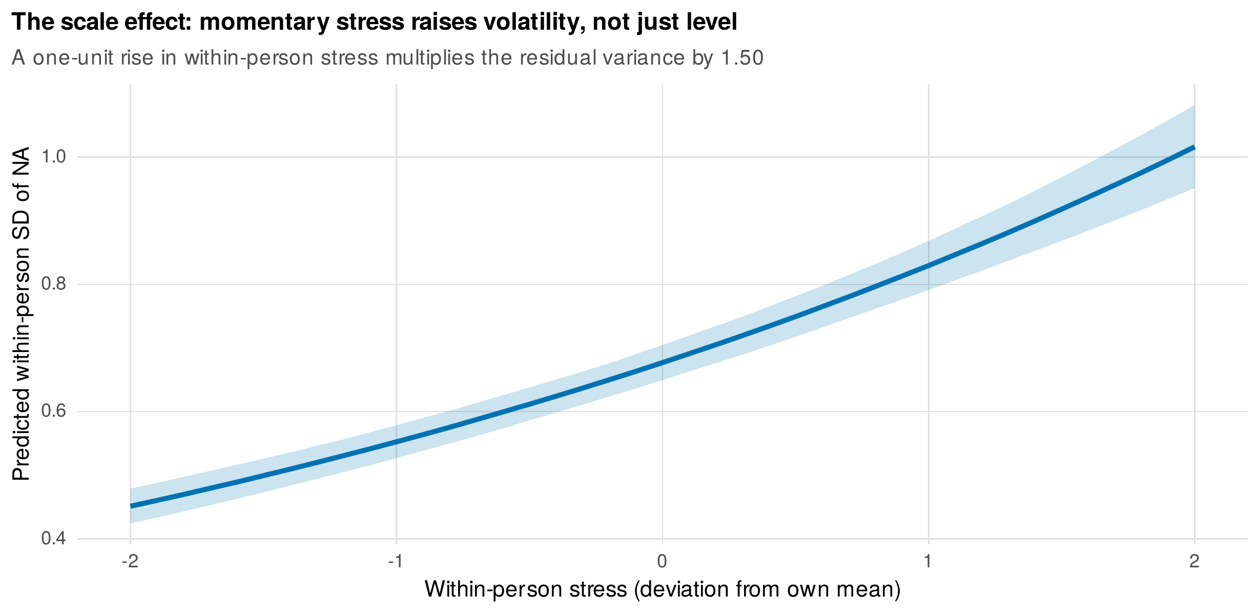
Note. Predicted within-person standard deviation of negative affect as a function of within-person stress, from the scale submodel, with a ninety-percent uncertainty band. A one-unit rise in momentary stress multiplies the residual variance by about \(1.5\). The scale submodel estimates this destabilizing effect separately from the effect of stress on the mean level.
The model repairs the two-stage index by shrinking the person-specific volatility estimates. Figure 16.5 compares each person’s raw log within-person standard deviation to the model’s empirical-Bayes estimate, plotted against the number of beeps. The raw estimates are extreme, especially for the persons with the fewest occasions, and the model pulls them toward the group in proportion to their unreliability, exactly the shrinkage of Chapter 13 now applied to a variance. That the shrunken estimates are better, not merely smoother, is checkable here because the truth is known: the model’s estimates of person volatility correlate \(0.90\) with the true random scale effects, against \(0.81\) for the raw indices. The location-scale correlation, the substantive target, is estimated at \(0.40\) with a standard error of \(0.10\), and Figure 16.6 shows the joint distribution of the person effects behind it: persons with a higher mean negative affect do tend to be more volatile in it. The wide standard error is itself a lesson. The location-scale correlation is estimated with far less precision than a mean effect, because it is a second-order quantity that depends on the spread of person volatilities, so studies aiming to estimate it need more persons and more occasions than studies aiming only at means, a power fact that connects to Chapter 4 and that honest reporting must acknowledge.
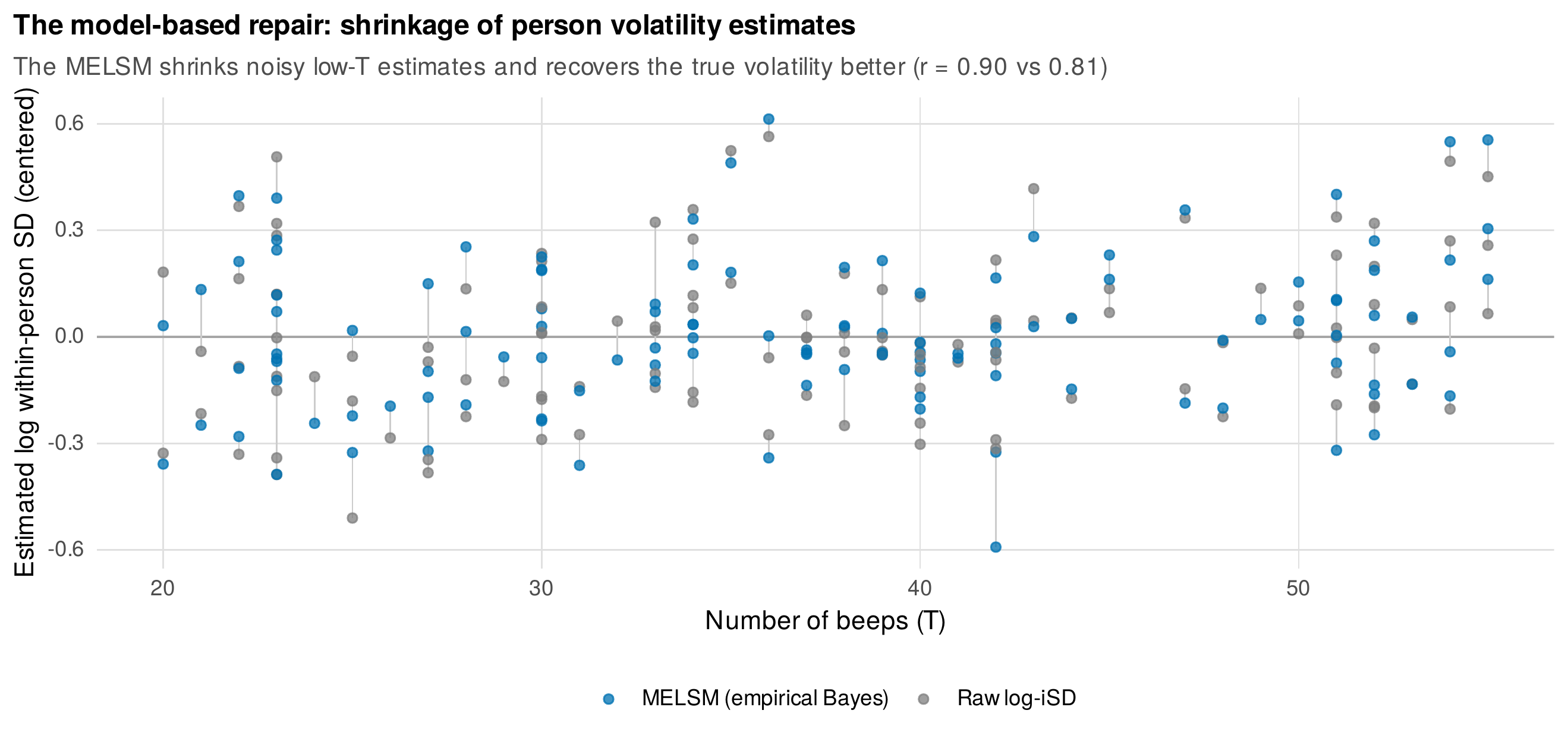
Note. Each person’s raw log within-person standard deviation (grey) and the model’s empirical-Bayes estimate (blue), joined by a segment, against the number of beeps. The model shrinks the noisy low-occasion estimates toward the group mean, and because the data-generating truth is known, the shrunken estimates can be shown to recover the true person volatility better than the raw indices (correlation \(0.90\) versus \(0.81\)).
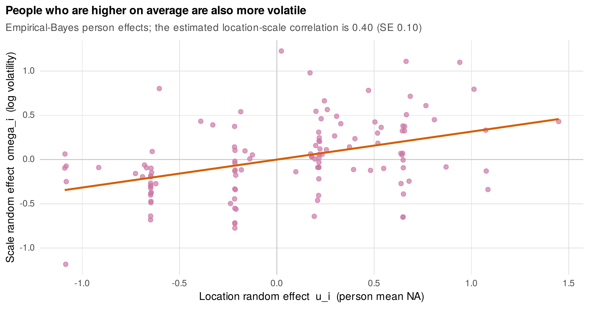
Note. The joint distribution of the empirical-Bayes location random effects (person mean) and scale random effects (person log volatility). The positive slope is the estimated location-scale correlation, here about \(0.40\) with a standard error of \(0.10\). This correlation, inaccessible to any two-stage analysis, is typically the substantive target of a location-scale study.
16.4 Extensions and Relatives
The scale submodel accepts the same elaborations as any regression, and two are especially useful. A predictor of variability may be time itself, turning the model into a statement about how volatility changes over a study. Figure 16.7 shows a variance trajectory in which within-person volatility declines across the weeks of a therapy, recovered by a time-varying scale model: variability is here a treatment outcome in its own right, the stabilization of a symptom rather than the reduction of its level, and a therapy might succeed on the second even where it is slow on the first. The distinction between between-person and within-person variance is the second elaboration. The random scale effect models between-person differences in volatility, while the scale covariates model within-person, occasion-to-occasion changes in it, and Hedeker’s framework separates the two explicitly (Hedeker et al., 2012). The multilevel machinery for individual differences in within-person variation predates the fully coupled model and remains a useful special case (Hoffman, 2007).
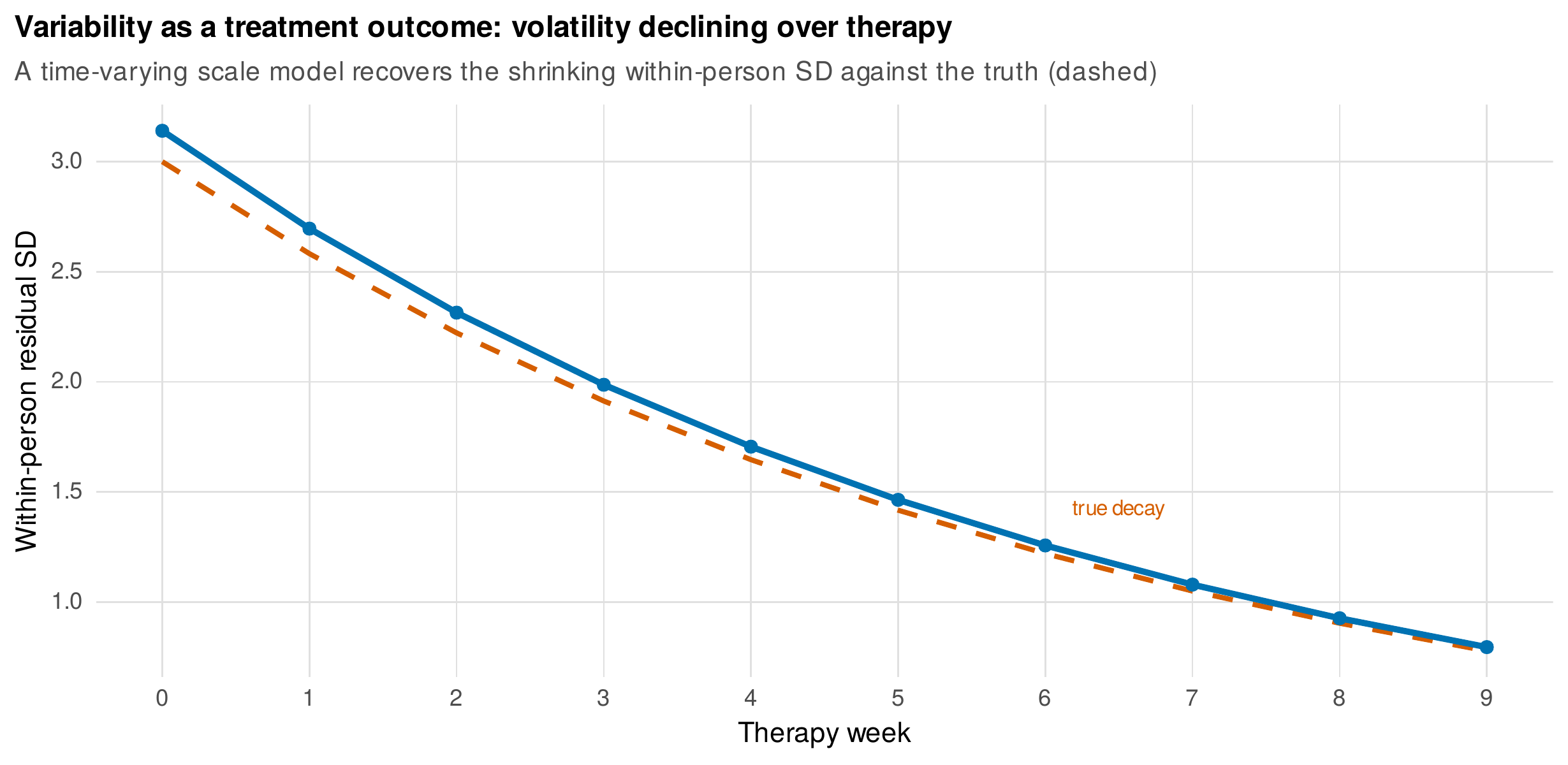
Note. A time-varying scale model in which the within-person residual standard deviation declines across therapy weeks. The fitted decay (blue) tracks the true generating decay (dashed). When variability itself is the outcome, its trajectory over an intervention is the finding, distinct from any change in the mean level.
The location-scale model sits within a family of distributional models that let parameters other than the mean depend on covariates. Table 16.3 maps the neighborhood. Double generalized linear models put a submodel on the dispersion of a generalized linear model; generalized additive models for location, scale, and shape allow every parameter of a flexible distribution, including skewness and kurtosis, to be a smooth function of covariates (Rigby & Stasinopoulos, 2005); variance-function mixed models and the dispersion formulas of modern software fit fixed scale submodels quickly; and the variance-modeling tradition in multilevel education research addresses the same structure from another field (Leckie et al., 2014). All share the premise that the spread, not only the center, is worth a model.
Table 16.3. The location-scale model among its distributional relatives.
| Model | What is modeled beyond the mean | R tool |
|---|---|---|
| Mixed-effects location-scale | Within-person variance, with a random scale effect | brms (distributional) |
| Double generalized linear model | Dispersion of a GLM | dglm |
| Variance-function GLMM | Residual dispersion, fixed | glmmTMB (dispformula) |
| GAMLSS | Location, scale, shape as smooth functions | gamlss |
Note. Distributional models let parameters other than the mean depend on covariates. The mixed-effects location-scale model is the member that adds a random scale effect for longitudinal data; the others trade the random scale for flexibility in the distributional form or for speed with fixed scale submodels.
A final extension concerns using the estimated variability downstream. When a person’s scale effect \(\omega_i\) is to serve as a predictor or an outcome in a further analysis, it must not be reduced to a point estimate and plugged in, because that discards its uncertainty and biases the second-stage result, the same plug-in fallacy that afflicts any use of a shrunken estimate as data. The correct practice carries the full posterior distribution of \(\omega_i\) forward, either by fitting the two stages jointly or by propagating draws, so that a person whose volatility is poorly estimated contributes proportionally less. This is one more reason the Bayesian route is natural here, since it produces the posterior draws that make honest propagation straightforward.
16.5 Validation, Pitfalls, and Reporting
A location-scale model must be checked where it makes its claims, on the variance structure, and the tool is a posterior predictive check aimed at variance features rather than at the mean. Figure 16.8 compares the observed distribution of per-person within-person standard deviations to the distribution replicated from the fitted model; the observed distribution falls comfortably within the replicated spread, evidence that the model reproduces the pattern of volatility it was built to explain. Checks of this kind, targeting the dispersion of the iSD across persons or the calibration of person-specific variances, are the location-scale analogue of the ordinary posterior predictive check and belong in any report. Table 16.4 is the reporting checklist, which extends the mixed-model checklist of Chapter 13 with the estimation-quality diagnostics that a Bayesian fit requires and that Chapter 17 explains in full.
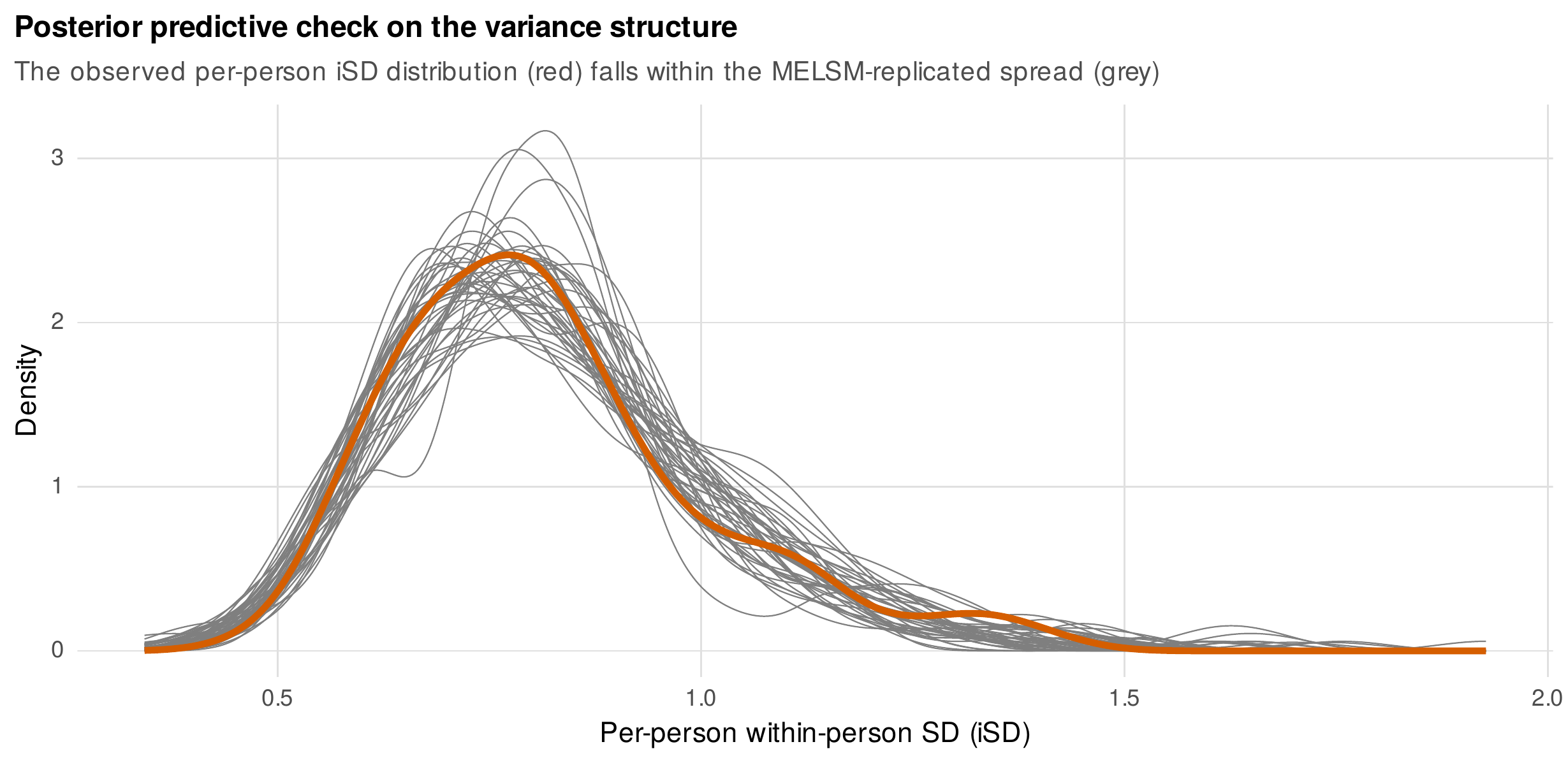
Note. The observed distribution of per-person within-person standard deviations (red) against forty distributions replicated from the fitted location-scale model (grey). The observed distribution lies within the replicated spread, indicating that the model reproduces the between-person pattern of volatility. Posterior predictive checks for a location-scale model should target variance features, not the mean.
Table 16.4. A reporting checklist for a mixed-effects location-scale model.
| Element | What to report |
|---|---|
| Location submodel | The mean-structure fixed and random effects |
| Scale submodel | The variance predictors, read multiplicatively, with the random scale variance |
| Location-scale correlation | The estimate with its uncertainty, and its substantive reading |
| Estimation | The engine and, for a Bayesian fit, the convergence diagnostics (\(\hat{R}\), effective sample size, divergences) |
| Design adequacy | The number of persons and occasions relative to the variance targets |
| Validation | Posterior predictive checks aimed at the variance structure |
Note. The scale submodel is reported on the multiplicative variance scale, and the location-scale correlation is reported with its full uncertainty, which is typically wide. The estimation diagnostics belong to the Bayesian machinery developed in Chapter 17.
Three pitfalls recur. Interpreting a scale coefficient as a raw standard-deviation effect ignores the log link and understates the effect; scale coefficients are multiplicative on the variance. Reading low variability off a bounded scale can be an artifact, because a person near a floor or ceiling has little room to vary, so an apparent difference in volatility may be a difference in level in disguise, the same caution the relative-standard-deviation discussion of Chapter 7 raised. And using a point estimate of a person’s volatility as an outcome launders away its uncertainty and biases the downstream analysis. Each is avoidable with the discipline the model itself supplies.
16.6 Fitting Location-Scale Models in R
The distributional-model syntax of brms states the two submodels in one formula, the first for the mean and a second, prefixed sigma, for the log standard deviation, each with its own fixed and random effects.
library(brms)
# Location: na ~ stress + (1 | person); Scale: log sigma ~ stress + (1 | person)
f <- bf(na    ~ stress_wc + (1 | p | person),
        sigma ~ stress_wc + (1 | p | person))   # shared "p": correlates the REs
m <- brm(f, data = ema, chains = 4, cores = 4)   # priors + MCMC; see Chapter 17
summary(m)                                        # scale effects are on log-SD
The shared grouping tag | p | is what correlates the location and scale random effects, yielding the location-scale correlation. A fixed-only scale model, without the random scale effect, is available more quickly through nlme residual-variance functions or the glmmTMB dispersion formula, useful as a stepping stone or when the random scale is not needed.
library(nlme)   # fixed log-linear scale: residual SD ~ exp(theta * stress)
m_fixed <- lme(na ~ stress_wc, random = ~1 | person, data = ema,
               weights = varExp(form = ~ stress_wc))
# glmmTMB alternative: glmmTMB(na ~ stress_wc + (1|person),
#                              dispformula = ~ stress_wc, data = ema)
The complete analysis, including the two-stage deficiency demonstration, the full location-scale model fitted by two-dimensional Gauss-Hermite maximum likelihood with empirical-Bayes person effects, the scale-effect and location-scale displays, the variance trajectory, and the variance-targeted posterior predictive check, is the shipped script ch16_analysis_V01.R, with figures drawn by ch16_figures_V01.R and the dataset generated by gen_ema_lability_V01.R. The script fits the model by maximum likelihood for transparency and portability; brms fits the same model by Markov chain Monte Carlo in a single call and is the recommended tool for applied work, especially when the scale submodel carries its own random slopes.
Software Note • tools for the location-scale model
Three families of tool fit the model. Hedeker’s MIXREGLS program and its successor MixWILD fit the mixed-effects location-scale model by maximum likelihood with adaptive quadrature and remain the reference implementations, with the additional capacity to let a random location effect enter the scale model, a feature few other tools offer; verify their current availability before relying on them. The Bayesian route through brms expresses the model as a distributional regression, generalizes to random scale slopes, three-level structures, and non-Gaussian locations, and produces the posterior draws that downstream propagation requires; it is this book’s default and the subject of Chapter 17. For a fixed-only scale model, nlme variance functions and the glmmTMB dispersion formula are fast and adequate. The gamlss package fits the broader location-scale-and-shape family for cross-sectional data.
16.7 Common Misconceptions
Several beliefs about within-person variability mislead. The first is that a well-estimated intraindividual standard deviation is as good as a model; it is not, because even with many occasions it lacks shrinkage, cannot carry covariates, and confounds level with variability whenever they are coupled. The second is that the scale submodel is a heteroscedasticity correction; here it is the hypothesis, and the within-person variance is the outcome of interest, not a nuisance to be swept away. The third is that variance findings are inherently less replicable; the truth is that they demand more of the design, more persons and more occasions, and their apparent fragility is usually a power problem that the honest planning of Chapter 4 addresses. The fourth is that a five-wave panel can support within-person variance modeling; it cannot, because a handful of occasions per person yields no usable estimate of that person’s volatility, and the method belongs to intensive designs.
Common Pitfall • three errors in location-scale practice
First, reading a scale coefficient as a raw-SD effect: the scale submodel is on the log variance, so a coefficient is a multiplicative factor on the variance, and reporting it as a difference in standard deviations understates it. Second, mistaking a floor for stability: on a bounded scale a person near the boundary cannot vary much, so low measured variability may be a level artifact, not genuine stability. Third, plugging in a point estimate of person volatility: using \(\hat{\omega}_i\) as data in a second analysis discards its uncertainty and biases the result; carry the posterior forward instead.
Chapter Summary
The mixed-effects location-scale model makes within-person variance a dependent variable. It answers questions, affective instability, performance inconsistency, symptom volatility, for which the spread is the phenomenon and the mean is beside the point (Figure 16.1). It repairs the four deficiencies of two-stage intraindividual standard deviations, their sampling noise, their lack of shrinkage, their confounding of level with variability, and their error-in-variables when used downstream (Figure 16.2, Table 16.1), by placing a log-linear submodel on the within-person variance, giving that submodel a random scale effect, and correlating the scale effect with the location effect (Figure 16.3, Table 16.2). Scale coefficients are read multiplicatively because the submodel is on the log variance (Figure 16.4), the person volatility estimates are shrunken and thereby recover the truth better than raw indices (Figure 16.5), and the location-scale correlation, the substantive target, links who is high to who is variable but is estimated with wide uncertainty (Figure 16.6). The scale submodel extends to a variance trajectory over time, making stabilization a treatment outcome (Figure 16.7), and the model sits within a family of distributional relatives (Table 16.3). Validation targets the variance structure through posterior predictive checks (Figure 16.8, Table 16.4), and the model’s estimation is the natural point at which Bayesian methods become necessary.
Where to Go Next
This chapter deliberately ends at the threshold of Bayesian estimation. The location-scale model is fit here by maximum likelihood for transparency, but its natural engine is Markov chain Monte Carlo, which handles the random scale slopes, the multilevel extensions, and the posterior propagation that maximum likelihood strains to provide. Chapter 17 supplies that machinery in full, and a reader who wants the recipe before the theory can fit the models of this chapter in brms now and return to Chapter 17 for the understanding. The within-person variance reappears throughout the intensive-longitudinal part of the book: Chapter 25 models heterogeneity in the innovation variance of a dynamic model, the moving cousin of the random scale effect, and Chapters 33 and 35 deploy affective instability as a clinical and personality construct. The lesson that the spread deserves a model, not only the center, recurs wherever a process is measured densely enough to reveal how much it swings.
Exercises
- 16.1 Deficiency demonstration. Simulate persons with unequal numbers of occasions and a common true volatility, and show that the ranking of persons by raw intraindividual standard deviation is unstable while the location-scale estimates, shrunken, are not.
- 16.2 Fit the scale submodel. On a diary outcome, fit a location-scale model with a within-person predictor in both submodels, and write the scale-submodel results paragraph, reporting the effect on the multiplicative variance scale.
- 16.3 A scale random slope. Extend the model to let the effect of the predictor on volatility vary across persons, assess convergence honestly, and report whether the data support the added complexity.
- 16.4 Variance-targeted checks. Propose and implement two posterior predictive checks aimed at the variance structure, and interpret what each would reveal about a misspecified scale submodel.
- 16.5 Location, scale, or both. For three research questions, decide whether each concerns the level, the variability, or their relationship, and specify the submodels that would answer it.
References
Bürkner, P.-C. (2017). brms: An R package for Bayesian multilevel models using Stan. Journal of Statistical Software, 80(1), 1–28. https://doi.org/10.18637/jss.v080.i01
Ebner-Priemer, U. W., Eid, M., Kleindienst, N., Stabenow, S., & Trull, T. J. (2009). Analytic strategies for understanding affective (in)stability and other dynamic processes in psychopathology. Journal of Abnormal Psychology, 118(1), 195–202. https://doi.org/10.1037/a0014868
Hedeker, D., Mermelstein, R. J., & Demirtas, H. (2008). An application of a mixed-effects location scale model for analysis of ecological momentary assessment (EMA) data. Biometrics, 64(2), 627–634. https://doi.org/10.1111/j.1541-0420.2007.00924.x
Hedeker, D., Mermelstein, R. J., & Demirtas, H. (2012). Modeling between-subject and within-subject variances in ecological momentary assessment data using mixed-effects location scale models. Statistics in Medicine, 31(27), 3328–3336. https://doi.org/10.1002/sim.5338
Hedeker, D., & Nordgren, R. (2013). MIXREGLS: A program for mixed-effects location scale analysis. Journal of Statistical Software, 52(12), 1–38. https://doi.org/10.18637/jss.v052.i12
Hoffman, L. (2007). Multilevel models for examining individual differences in within-person variation and covariation over time. Multivariate Behavioral Research, 42(4), 609–629. https://doi.org/10.1080/00273170701710072
Hultsch, D. F., MacDonald, S. W. S., & Dixon, R. A. (2002). Variability in reaction time performance of younger and older adults. The Journals of Gerontology: Series B, Psychological Sciences and Social Sciences, 57(2), P101–P115. https://doi.org/10.1093/geronb/57.2.P101
Jahng, S., Wood, P. K., & Trull, T. J. (2008). Analysis of affective instability in ecological momentary assessment: Indices using successive difference and group comparison via multilevel modeling. Psychological Methods, 13(4), 354–375. https://doi.org/10.1037/a0014173
Leckie, G., French, R., Charlton, C., & Browne, W. (2014). Modeling heterogeneous variance-covariance components in two-level models. Journal of Educational and Behavioral Statistics, 39(5), 307–332. https://doi.org/10.3102/1076998614546494
Rast, P., Hofer, S. M., & Sparks, C. (2012). Modeling individual differences in within-person variation of negative and positive affect in a mixed effects location scale model using BUGS/JAGS. Multivariate Behavioral Research, 47(2), 177–200. https://doi.org/10.1080/00273171.2012.658328
Rigby, R. A., & Stasinopoulos, D. M. (2005). Generalized additive models for location, scale and shape. Journal of the Royal Statistical Society: Series C (Applied Statistics), 54(3), 507–554. https://doi.org/10.1111/j.1467-9876.2005.00510.x
Wang, L., Hamaker, E. L., & Bergeman, C. S. (2012). Investigating inter-individual differences in short-term intra-individual variability. Psychological Methods, 17(4), 567–581. https://doi.org/10.1037/a0029317
Williams, D. R., Zimprich, D. R., & Rast, P. (2019). A Bayesian nonlinear mixed-effects location scale model for learning. Behavior Research Methods, 51(5), 1968–1986. https://doi.org/10.3758/s13428-019-01255-9