Chapter 17
Bayesian Estimation for Longitudinal Models
The preceding chapters kept arriving at the same door. The mixed model of Chapter 13 met boundary estimates and singular fits where a variance collapsed to zero. The generalized linear mixed model of Chapter 15 needed to integrate random effects out of a likelihood that had no closed form. The location-scale model of Chapter 16 placed a random effect inside a variance and correlated it with the mean, straining maximum likelihood past comfort. Each difficulty has a common resolution, and this chapter supplies it. Bayesian estimation treats the parameters as uncertain quantities with probability distributions, combines a prior with the likelihood to obtain a posterior, and explores that posterior by simulation rather than by maximizing a function. This is not a chapter of Bayesian philosophy, and it takes no side in old debates. It is a working chapter that frames Bayesian methods as three practical things: an estimation rescue for models that defeat maximum likelihood, a principled route to inference when samples are small, and the natural language for propagating uncertainty into derived quantities and predictions. The reader should leave bilingual, able to use Bayesian estimation where it helps and to defend either engine on its merits.
Learning Objectives
After working through this chapter, you should be able to: (1) state how a posterior is formed from a prior and a likelihood, and interpret posteriors, credible intervals, and posterior predictive distributions; (2) choose priors for longitudinal parameters, especially variance components and correlations, and check them by prior predictive simulation; (3) run and diagnose Markov chain Monte Carlo using the split \(\hat{R}\), effective sample size, and divergence diagnostics, and recognize the funnel pathology and its non-centered cure; (4) criticize a model with posterior predictive checks and compare models with cross-validation; (5) reproduce the book’s earlier models under Bayesian estimation and say when the answers should and should not differ from maximum likelihood; and (6) exploit the distinctly Bayesian payoffs of boundary-free variance estimation, honest small-sample inference, and full uncertainty on derived quantities.
17.1 The Inferential Frame, Minimally
Bayesian inference rests on one identity. The posterior distribution of the parameters given the data is proportional to the likelihood of the data given the parameters times the prior distribution of the parameters, \(p(\bm{\theta}\mid \mathbf{y}) \propto p(\mathbf{y}\mid \bm{\theta})\,p(\bm{\theta})\). The likelihood is the same object that maximum likelihood maximizes, the prior encodes what is known about the parameters before seeing the data, and the posterior is the updated state of knowledge after. Figure 17.1 shows the three objects for a single parameter, the average slope of the sleepstudy reaction-time data. A weakly informative prior, broad relative to the plausible range, contributes little; the likelihood carries the information in the data; and the posterior sits almost on top of the likelihood, nudged only slightly toward the prior. This is the usual situation with informative data and weak priors: the posterior is data-dominated, and the prior serves mainly to regularize rather than to steer. When the data are sparse or the parameter weakly identified, the prior does more work, which is why the choice of prior receives its own section below.
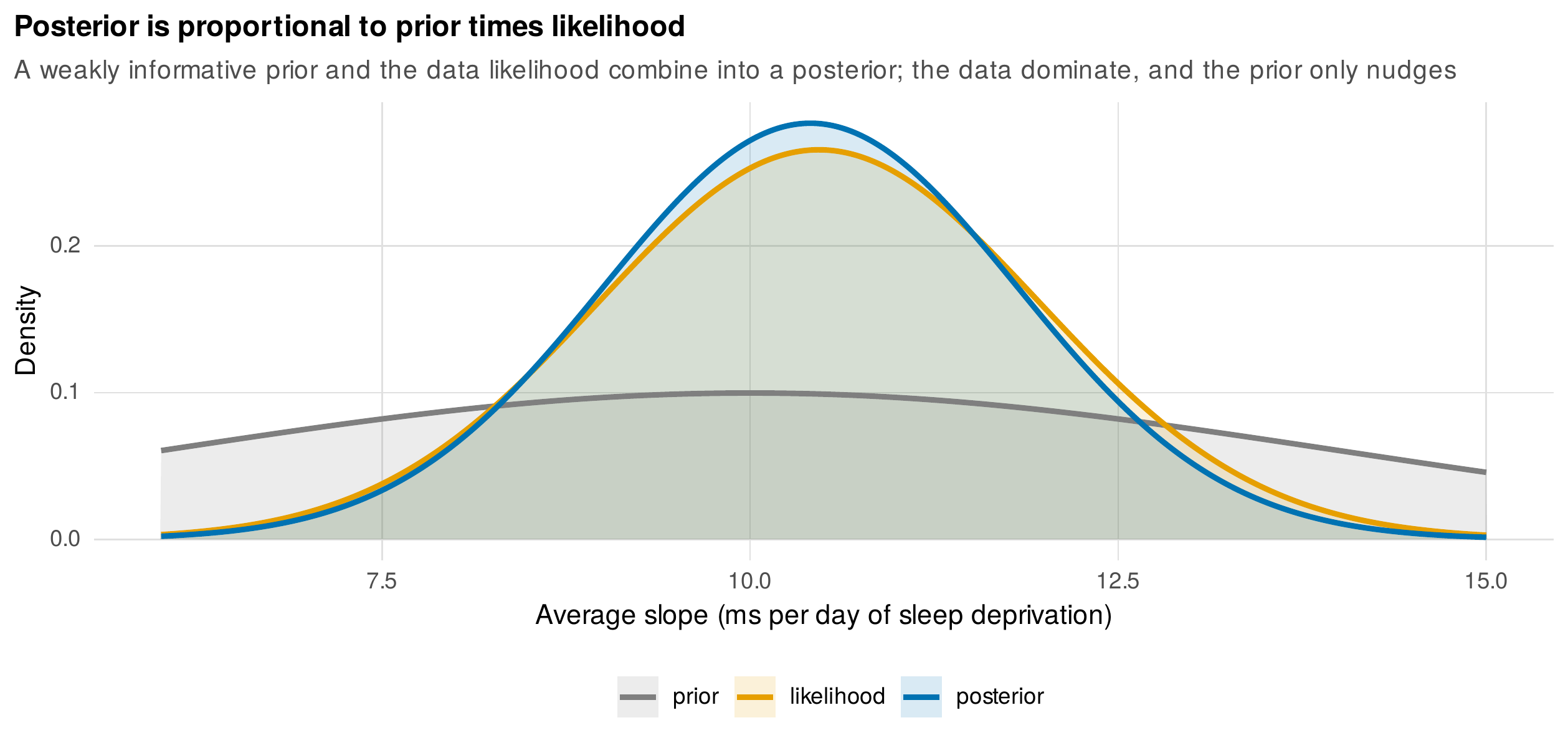
Note. For the average slope of the sleepstudy data, a weakly informative prior (grey), the data likelihood (orange), and the resulting posterior (blue). The posterior is a precision-weighted compromise, here almost coincident with the likelihood because the data are informative and the prior is weak. When data are sparse the prior contributes more, which is why priors must be chosen and checked.
The product of this machinery is a full distribution for every parameter, and inference reads quantities off that distribution directly. A credible interval is an interval that contains the parameter with a stated posterior probability, and it means exactly what newcomers wrongly assume a confidence interval means: given the data, model, and prior, there is a ninety-five-percent probability that the parameter lies in the ninety-five-percent credible interval. A confidence interval makes the subtler frequentist statement about the long-run coverage of the procedure, not about this interval. The two are numerically similar under weak priors and ample data and diverge when priors are informative or samples small, and the difference is in what is treated as random: the parameter, for the Bayesian, or the interval, for the frequentist. This book’s use of Bayesian methods is oriented toward estimation and prediction, reporting posteriors and credible intervals for parameters and predictive distributions for new observations, and it defers the Bayes-factor apparatus for hypothesis testing to a brief and cautionary treatment later in the chapter.
The reason longitudinal modeling keeps arriving at Bayesian estimation is worth stating as a map. Chapter 13 met variance parameters on the boundary of their space, where the maximum-likelihood estimate is a degenerate point and its uncertainty is ill-defined. Chapter 15 met intractable integrals over random effects. Chapter 16 met a random effect inside a variance. The parts to come compound these: the latent-variable dynamics of Part VI, the continuous-time and state-space models, and the dynamic structural equation models are in practice estimated by Markov chain Monte Carlo because no other method handles their weakly identified, high-dimensional posteriors gracefully. This chapter is therefore placed as the estimation engine of the book, built once and consumed repeatedly.
17.2 Priors for Longitudinal Parameters
A prior is a modeling choice, and like any modeling choice it must be deliberate and checked. For fixed effects the standard recommendation is a weakly informative prior on a standardized scale, a normal distribution wide enough to be uninformative about the sign and rough magnitude of an effect but narrow enough to rule out absurd values, which stabilizes estimation without materially influencing the posterior when data are adequate. The interesting priors in longitudinal models are on the variance components and the correlations, and here recent practice has shifted decisively away from old defaults.
The historical default for a variance was the inverse-gamma distribution, chosen for conjugacy, but it behaves badly precisely where longitudinal models live, near zero, because a variance component that is genuinely small is pushed away from zero by an inverse-gamma prior in a way that is hard to make uninformative (Gelman, 2006). The modern recommendation places the prior on the standard deviation rather than the variance, and uses a half-normal or half-t distribution, densities that are largest at zero and decay smoothly, so that a small or zero variance is allowed rather than forbidden. This is the boundary story of Chapter 13 retold as a prior: where maximum likelihood collapsed a small variance to exactly zero, a half-normal prior lets the posterior concentrate near zero while keeping its uncertainty. What makes such a prior weakly informative is not a slogan but a checkable implication, and the check is prior predictive simulation: draw parameters from the prior, and inspect the data or the derived quantities they imply. Figure 17.2 performs this check for the intraclass correlation implied by three variance priors. A half-normal with a large scale, intended to be uninformative, in fact piles prior mass near zero and one, an implausible prior belief that most of the variance is either all within or all between clusters; a tighter half-normal spreads the implied intraclass correlation more evenly; and a half-Cauchy places heavy mass at the extremes. The lesson is that a prior on a variance is a prior on everything the variance implies, and only prior predictive simulation reveals what has actually been assumed.
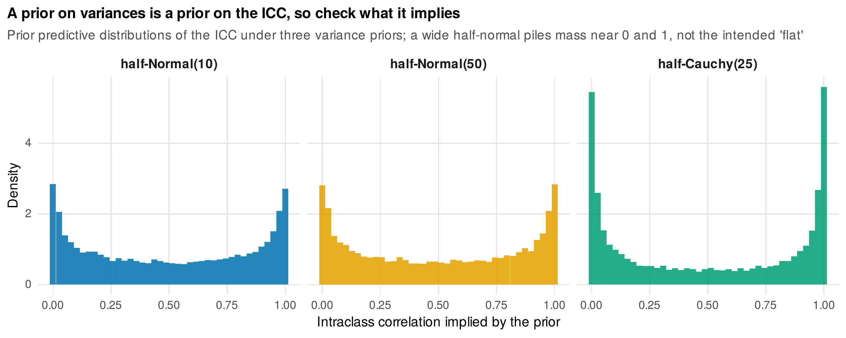
Note. Prior predictive distributions of the intraclass correlation implied by three priors on the random-effect and residual standard deviations. A wide half-normal, meant to be uninformative, implies a prior belief that the intraclass correlation is near zero or one; a tighter half-normal is more even; a half-Cauchy favors the extremes. The implied distribution, not the nominal width, is what makes a variance prior weakly informative.
Correlations among random effects, the off-diagonal of the T matrix of Chapter 13, receive a prior of their own. The standard choice is the LKJ prior on the correlation matrix (Lewandowski et al., 2009), governed by a single shape parameter \(\eta\), and Figure 17.3 shows its behavior for a single correlation. At \(\eta=1\) the prior is flat over the legal range, at \(\eta\) greater than one it concentrates toward zero and so regularizes correlations toward independence, and at \(\eta\) less than one it favors the extremes. A mild value such as \(\eta=2\) is a sensible default, expressing a weak belief that random effects are not perfectly correlated while letting the data speak. Prior sensitivity is then a routine part of the workflow rather than an afterthought: the model is refit under two or three defensible prior sets, and the posterior conclusions are reported as robust only if they survive. Informative priors drawn from prior studies are legitimate and valuable when the earlier evidence is sound, with the standing caution that a literature distorted by publication bias will supply priors that are too confident and too far from zero. Table 17.1 collects the default recommendations.
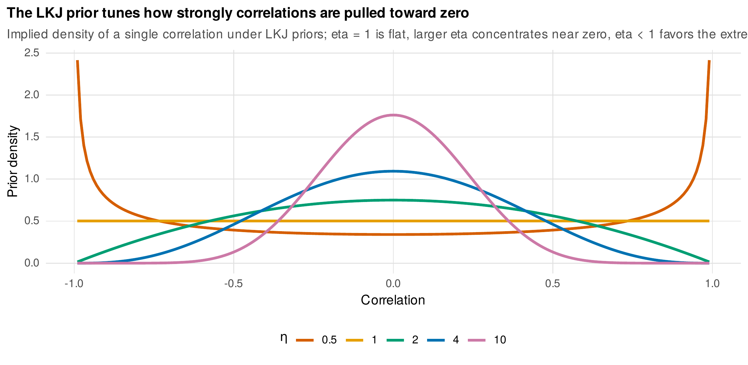
Note. The prior density of a single random-effect correlation under the LKJ prior for several values of the shape parameter \(\eta\). At \(\eta=1\) the prior is flat; larger \(\eta\) concentrates the correlation near zero, regularizing toward independence; \(\eta\) below one favors strong correlations. A value near \(\eta=2\) is a common weakly informative default.
Table 17.1. Default weakly informative priors by parameter class.
| Parameter | Recommended prior | Prior predictive check |
|---|---|---|
| Fixed effect | Normal on a standardized scale | Implied effect magnitudes |
| Random-effect SD | Half-normal or half-t on the SD | Implied intraclass correlation |
| Residual SD | Half-normal or half-t on the SD | Implied outcome spread |
| Correlation matrix | LKJ with \(\eta \approx 2\) | Implied correlation density |
Note. Priors are placed on standard deviations, not variances, to avoid the boundary pathology of the inverse-gamma. Every prior is checked by simulating from it and inspecting the implied data or derived quantities, not by trusting its nominal width.
17.3 Markov Chain Monte Carlo in Practice
The posterior is known only up to a constant and cannot in general be summarized analytically, so it is explored by simulation. Markov chain Monte Carlo constructs a chain of parameter draws whose stationary distribution is the posterior, so that after an initial warmup the draws are samples from the posterior and any quantity of interest is estimated by averaging over them. The modern default algorithm is Hamiltonian Monte Carlo and its self-tuning variant, the no-U-turn sampler, which uses the gradient of the log posterior to propose distant, informed moves and so explores correlated high-dimensional posteriors far more efficiently than the random-walk and Gibbs samplers of earlier practice (Betancourt, 2017). The practical defaults are several chains run from different starting points, a warmup phase discarded, and enough post-warmup iterations to estimate the quantities of interest with acceptable precision; the number is raised when the diagnostics below demand it.
Foundations Box • Why gradients help, and how cross-validation is approximated
Hamiltonian Monte Carlo augments the parameters with auxiliary momentum variables and simulates the physics of a particle sliding along the log-posterior surface, so that a single proposal follows the contours of the distribution for a long trajectory rather than taking a blind local step. Because the trajectory respects the geometry, the sampler moves quickly across a correlated posterior that would trap a random walk, and the price is that it requires the gradient of the log posterior, which probabilistic programming languages compute automatically. The same posterior draws support model comparison through leave-one-out cross-validation, which asks how well the model predicts each observation when that observation is held out. Refitting the model once per observation would be prohibitive, so the held-out predictive density is approximated from the single full fit by importance sampling, reweighting the posterior draws to represent the leave-one-out posterior, with a diagnostic (the Pareto shape) that flags observations for which the approximation is unreliable and which are usually the influential ones (Vehtari et al., 2017).
A fitted chain must be diagnosed before it is trusted, and four diagnostics do most of the work. The potential scale reduction factor, \(\hat{R}\), compares the variance within chains to the variance between chains; when the chains have converged to the same distribution the two agree and \(\hat{R}\) is near one, and a value above roughly \(1.01\) signals that the chains have not mixed (Vehtari et al., 2021). Figure 17.4 shows the visual counterpart: healthy chains overlap and interleave like white noise around a common level, while pathological chains started from different points have not met after equal effort, and their separation is the geometry behind a large \(\hat{R}\), here \(6.63\) against the healthy \(1.08\). The effective sample size measures how many independent draws the autocorrelated chain is worth, in bulk for the center of the distribution and in the tail for its extremes, and a small effective sample size means the posterior summaries are themselves noisy. Divergent transitions are failures of the Hamiltonian simulation that signal a region the sampler cannot traverse, and they are the diagnostic most specific to longitudinal models, because they arise from the funnel geometry that hierarchical models create. Table 17.2 states each diagnostic, its threshold, the pathology it detects, and its remedy.
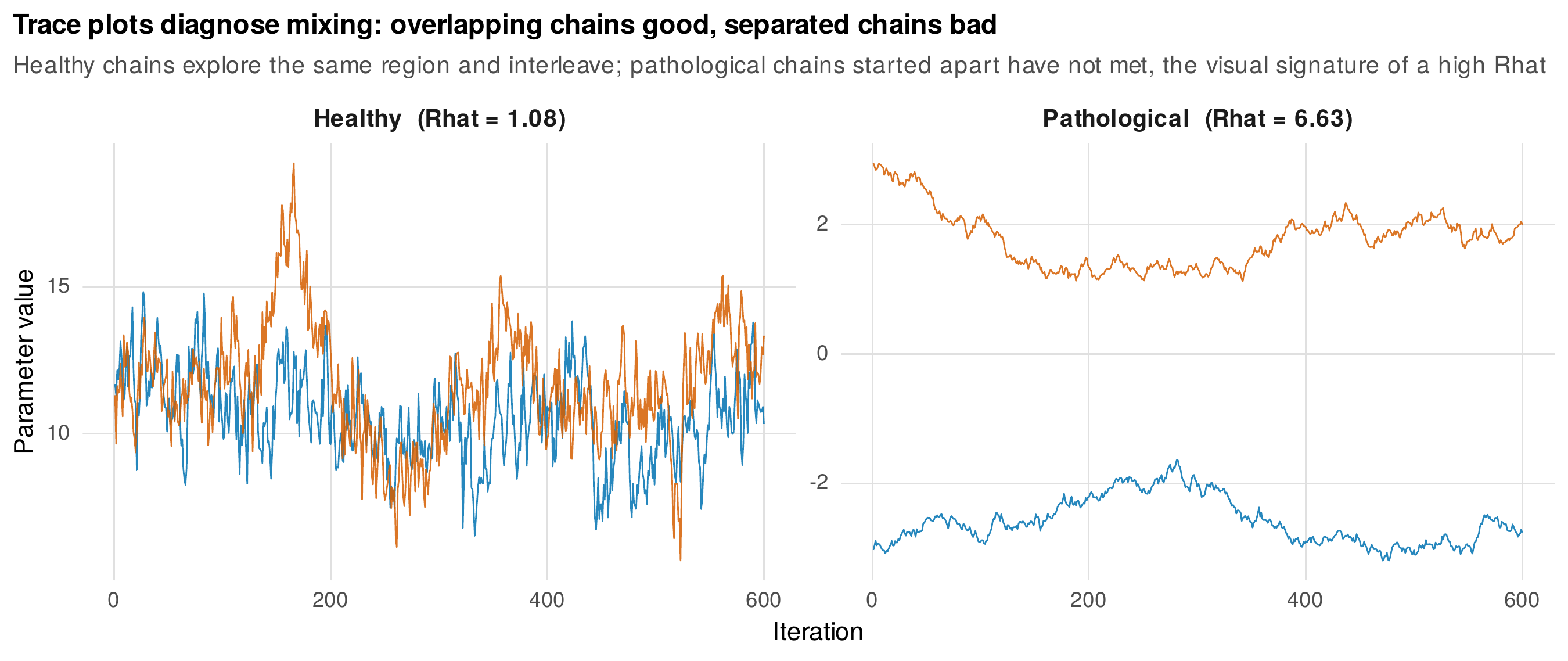
Note. Left: healthy chains for a well-identified parameter, overlapping and interleaving around a common level, with \(\hat{R}\) near one. Right: pathological chains started from different points that have not converged to a common distribution after equal effort, the visual signature of a large \(\hat{R}\). A trace plot is the first and fastest convergence diagnostic.
Table 17.2. The Markov chain Monte Carlo diagnostic quartet.
| Diagnostic | Threshold | Pathology | Remedy |
|---|---|---|---|
| \(\hat{R}\) | Below about \(1.01\) | Chains not mixed | More iterations; better parameterization |
| Effective sample size | Hundreds, bulk and tail | Noisy summaries | More iterations; reparameterize |
| Divergent transitions | None | Unreachable geometry (funnel) | Non-centered parameterization; raise adapt target |
| Maximum tree depth | Not saturated | Inefficient trajectories | Reparameterize; raise the limit |
Note. The four diagnostics are checked together, because each detects a different failure. Divergences are the most consequential for hierarchical longitudinal models and must never be ignored: they signal bias, not merely inefficiency.
The funnel deserves its own picture because it is the characteristic pathology of hierarchical models and the reason a well-specified model can still fail to fit. When a group-level standard deviation is itself a parameter, the joint posterior of that log standard deviation and the group effects it governs has a funnel shape: where the standard deviation is small the group effects are squeezed into a narrow neck, and where it is large they spread into a wide mouth. Figure 17.5 draws it. In the neck the conditional spread of the group effects collapses, in the running example from about \(4.5\) at the mouth to about \(0.2\) in the neck, a more than twentyfold change in scale that no single step size can match, so a gradient sampler tuned to the mouth overshoots the neck and diverges. The cure is not a tuning knob but a change of variables. The non-centered parameterization rewrites each group effect as the group standard deviation times a standard-normal auxiliary variable, which uncouples the two and turns the funnel into the benign, uncorrelated blob in the right panel of the figure. The model is unchanged; only its coordinates differ, and modern software applies the reparameterization by default while still surfacing divergences when they remain. Reparameterization intuition of this kind, recognizing when a model’s geometry rather than its specification is the problem, is the single most useful skill for fitting hierarchical models by Markov chain Monte Carlo.
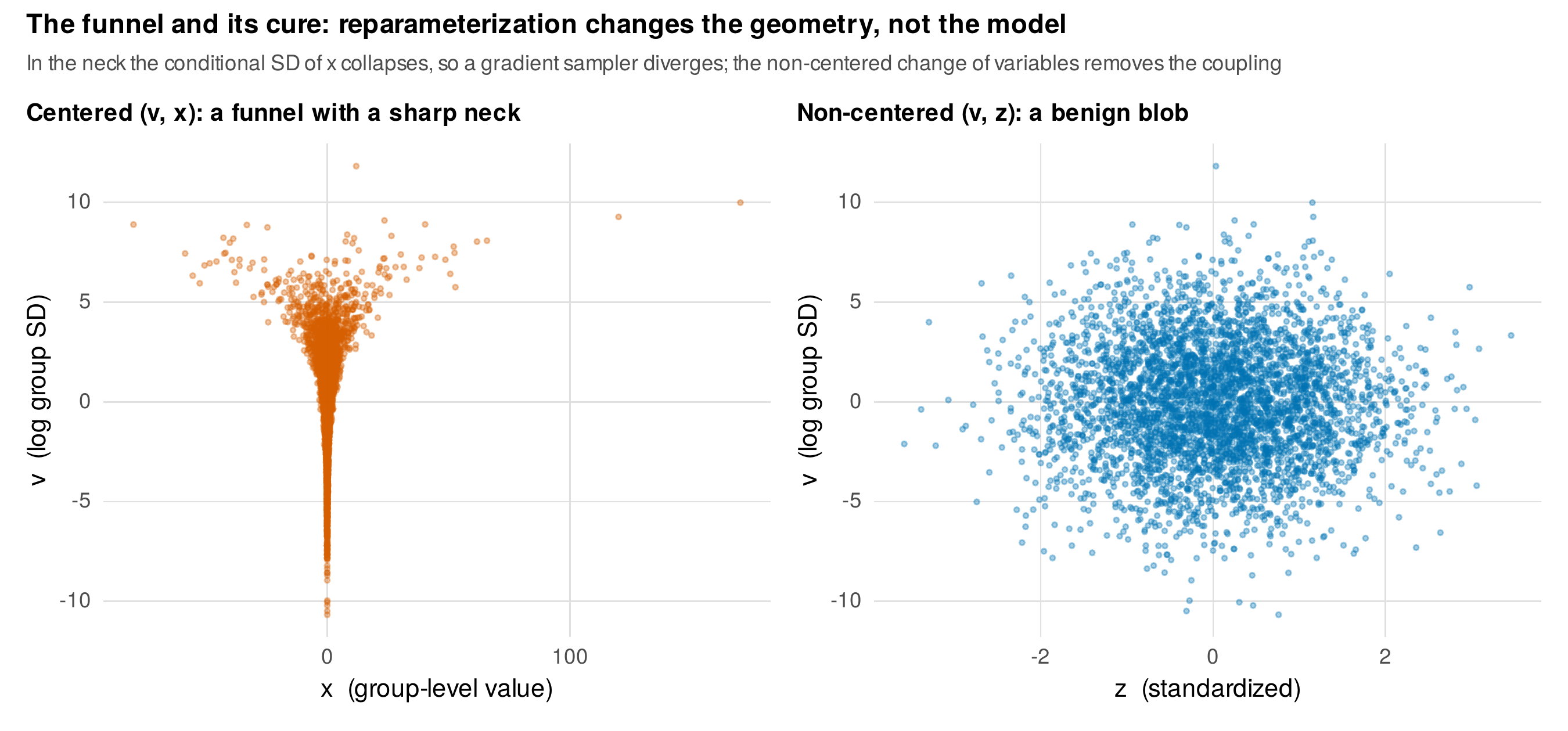
Note. Left: in the centered coordinates of a group log standard deviation and a group effect, the posterior is a funnel whose neck the sampler cannot traverse, because the conditional spread of the group effect collapses there. Right: the non-centered coordinates, in which the group effect is written as the standard deviation times a standard-normal variable, uncouple the axes into a benign blob. The two describe the same model.
17.4 Model Criticism and Comparison
A Bayesian model is criticized by posterior predictive checking: data are simulated from the fitted model, and features of the simulated data are compared to the same features of the observed data. If the model is adequate the observed data look like a plausible draw from it, and if some feature is systematically off the discrepancy localizes the misspecification. The art is in choosing the features to check, which should be the quantities the model must get right for its intended use, the mean trajectory over time, the spread of individual trajectories, or the variance structure that Chapter 16 modeled explicitly. Figure 17.6 checks the mean trajectory of the sleepstudy model: the observed daily means fall within the posterior predictive band, so the model reproduces the average structure. A check aimed at the variance, or at the person-level trajectories, would interrogate other commitments, and a thorough report assembles a small gallery of such checks rather than relying on one.
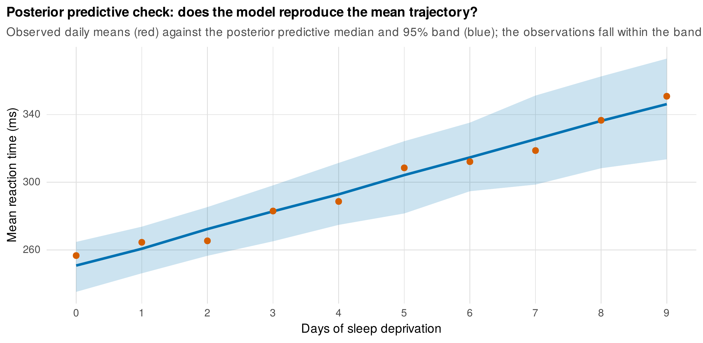
Note. Observed daily mean reaction times (red) against the posterior predictive median and ninety-five-percent band (blue) from the fitted model. The observations fall within the band, evidence that the model reproduces the mean trajectory. Posterior predictive checks are chosen to target the features the model must get right for its purpose.
Models are compared by their expected predictive accuracy for new data, estimated by leave-one-out cross-validation or the closely related widely applicable information criterion, both computed from the posterior draws. What these tools estimate is out-of-sample predictive performance, not truth: the model they favor is the one expected to predict a new observation best, which is not necessarily the one that describes the mechanism, a distinction that matters wherever prediction and explanation diverge and that Chapter 31 develops. Their diagnostic, the Pareto shape for each observation, flags points for which the approximation is unreliable, and those points are typically the influential and substantively interesting ones, a person whose trajectory the model struggles to accommodate. Table 17.3 sets the comparison tools side by side. Bayes factors, which compare the marginal likelihoods of two models, answer a genuinely different question, the relative evidence for one model over another, but they are notoriously sensitive to the priors on the parameters, including priors that were harmless for estimation, and they require specialized computation. They have their uses, but this book’s default for model comparison is predictive, through cross-validation, supplemented by the substantive judgment that no automatic criterion can replace.
Table 17.3. Tools for comparing Bayesian models.
| Tool | Question answered | Caution |
|---|---|---|
| Leave-one-out cross-validation | Out-of-sample predictive accuracy | Pareto-\(k\) flags influential points |
| Widely applicable information criterion | Out-of-sample predictive accuracy | Less robust than leave-one-out |
| Bayes factor | Relative evidence for one model | Highly sensitive to parameter priors |
| Posterior predictive check | Does the model reproduce key features | A check, not a score |
Note. Cross-validation and the information criterion estimate prediction, not truth, and the model they favor need not be the explanatory one. Bayes factors answer an evidential question but depend strongly on priors. Predictive comparison plus posterior predictive checking is this book’s default.
17.5 The Payoffs, Demonstrated
Three demonstrations show what Bayesian estimation buys, each closing with an honest note on where maximum likelihood remains preferable. The first is a boundary rescue. On a small dataset of eight persons, a random-slope model fit by restricted maximum likelihood returns a singular fit, collapsing the slope standard deviation to the boundary at zero and reporting no uncertainty for it, the pathology of Chapter 13. The Bayesian fit of the same model, with a half-normal prior on the slope standard deviation, returns a posterior that concentrates near zero but stays away from it and carries a wide credible interval, from about \(0.03\) to \(2.42\) in the running example. Figure 17.7 contrasts the two. The Bayesian answer is not that the slope variance is large; it is that the data cannot resolve it, and the posterior says so honestly rather than collapsing to a false certainty. Downstream, any quantity that depends on the slope variance inherits this honest uncertainty rather than a point at the boundary.
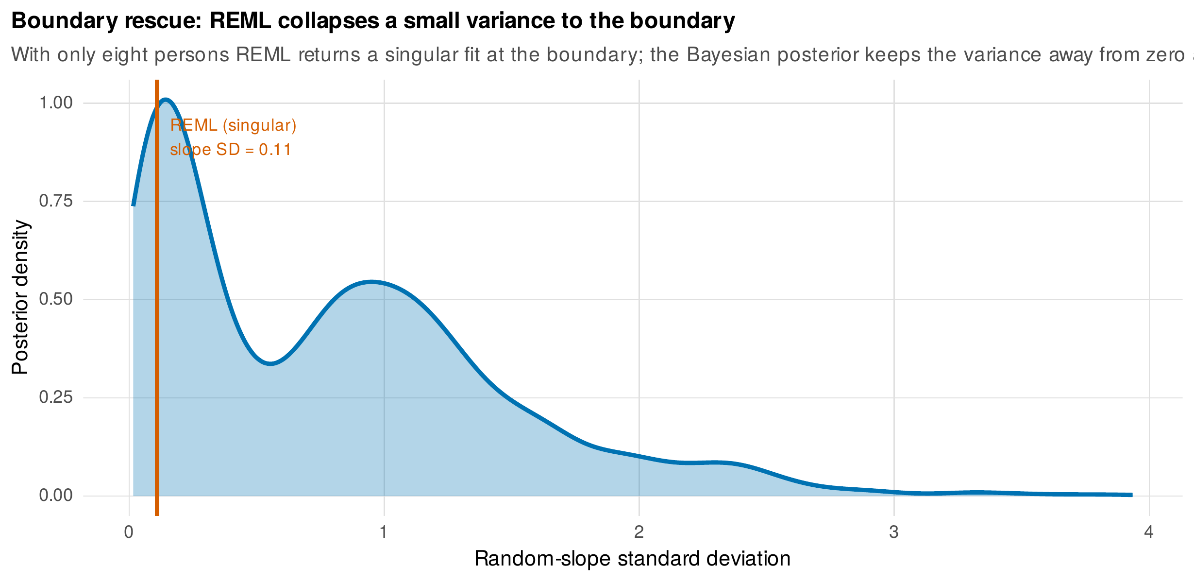
Note. For a random-slope model on eight persons, restricted maximum likelihood returns a singular fit with the slope standard deviation at the boundary (red line), and no uncertainty. The Bayesian posterior (blue) keeps the standard deviation away from zero and carries a wide credible interval, expressing honestly that the data cannot resolve the variance rather than collapsing it.
The second payoff is small-sample inference. When the number of clusters is small, the frequentist interval for a fixed effect based on the naive normal approximation under-covers, because it ignores the uncertainty in the estimated variance components, the same problem the Satterthwaite and Kenward-Roger corrections of Chapter 13 address. Figure 17.8 summarizes a simulation with only five clusters: the naive interval covers the true value in about eighty-nine percent of samples against a nominal ninety-five, while the Bayesian credible interval, wider because it integrates over the uncertainty in the variances, covers in about ninety-three percent. The Bayesian interval is better calibrated at small samples not by magic but by honesty about what is unknown, and the caution, developed below, is that this honesty depends on sensible priors; a careless prior can make small-sample Bayesian inference worse, not better (McNeish, 2016; Smid et al., 2020).
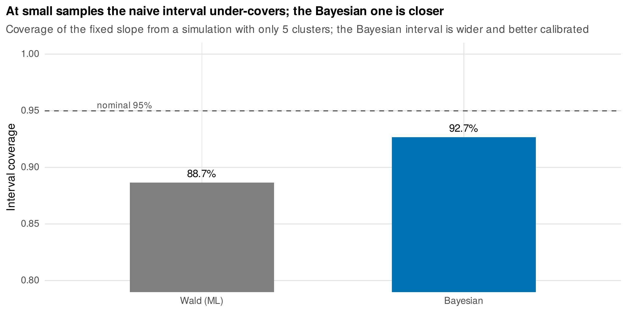
Note. Coverage of the nominal ninety-five-percent interval for a fixed slope, from a simulation with only five clusters. The naive maximum-likelihood interval under-covers because it ignores uncertainty in the variance components; the Bayesian credible interval, wider, is closer to nominal. The improvement depends on reasonable priors, not on the label.
The third payoff is uncertainty propagation. Because Bayesian estimation returns draws from the joint posterior, any function of the parameters inherits a full posterior distribution for free, including quantities that maximum-likelihood point machinery can only approximate awkwardly. Figure 17.9 shows one such derived quantity: for each person in the sleepstudy data, the posterior probability that their true slope is negative, that is, that their reaction time improves rather than worsens under sleep deprivation. Almost no person has an appreciable probability of improvement, and the one whose estimate is most ambiguous carries a probability near one half, with all of this uncertainty properly quantified. Questions of this form, the probability that a person belongs to a category, the proportion of a population with a declining trajectory, the predicted path of a not-yet-observed individual, are answered directly from the posterior draws, whereas maximum likelihood must resort to the delta method or the bootstrap and still struggles to propagate the uncertainty in the variance components. Figure 17.10 then makes the balanced point that closes each demonstration: across the parameters of the refit sleepstudy model, the maximum-likelihood estimate and the Bayesian posterior mean agree closely, the variance components being only slightly larger under the Bayesian fit because it does not share maximum likelihood’s downward bias. The two engines usually return the same numbers; they differ in what they treat as uncertain and in what they can honestly say when the data are thin. Table 17.4 lays out when each is preferable for this book’s model families.
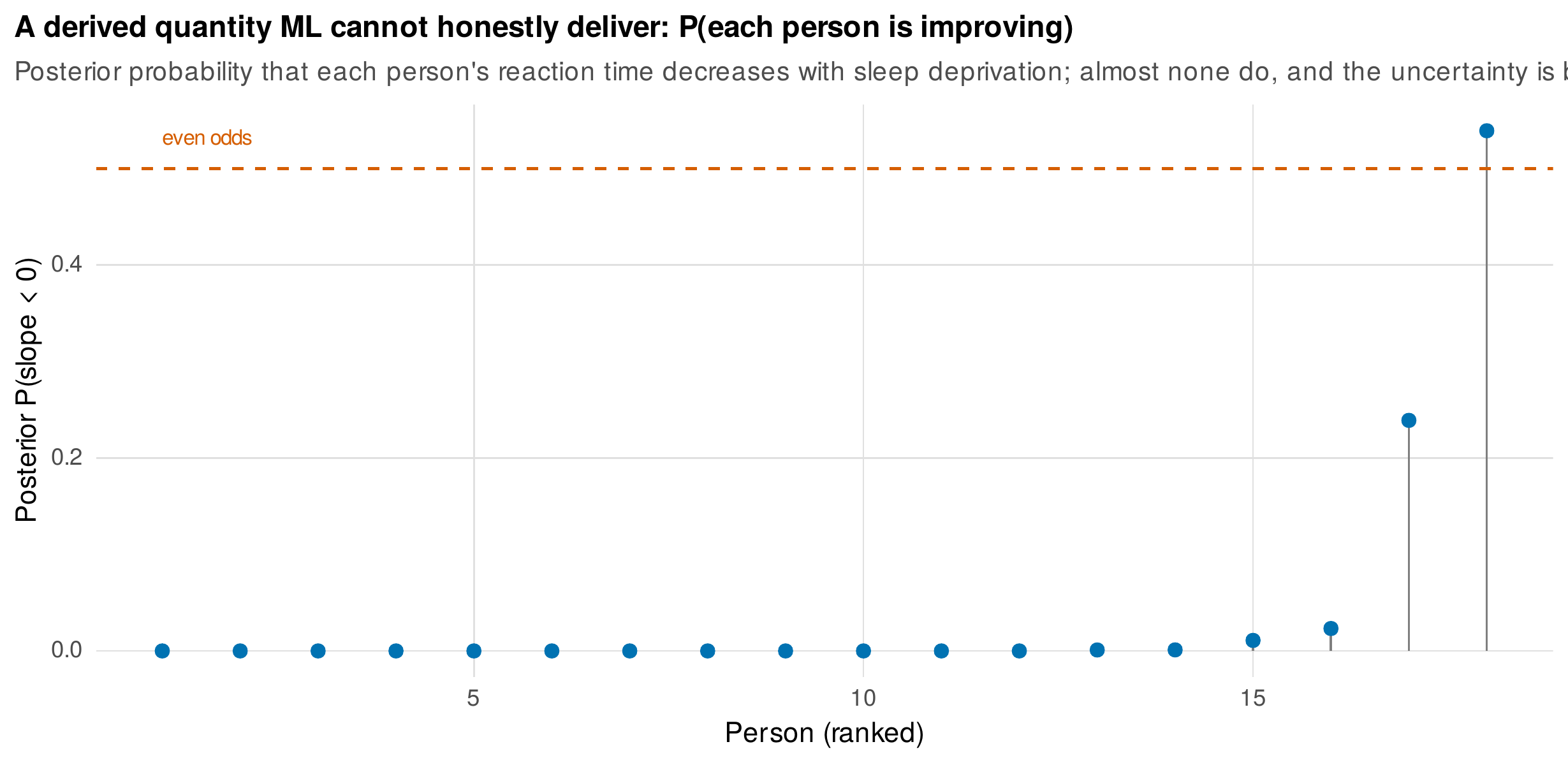
Note. For each person in the sleepstudy data, the posterior probability that their true slope is negative, that reaction time improves under sleep deprivation. Almost none do, and the most ambiguous person sits near even odds. Such person-level derived quantities, with their uncertainty, follow directly from the posterior draws and are awkward to obtain honestly from maximum-likelihood point estimates.
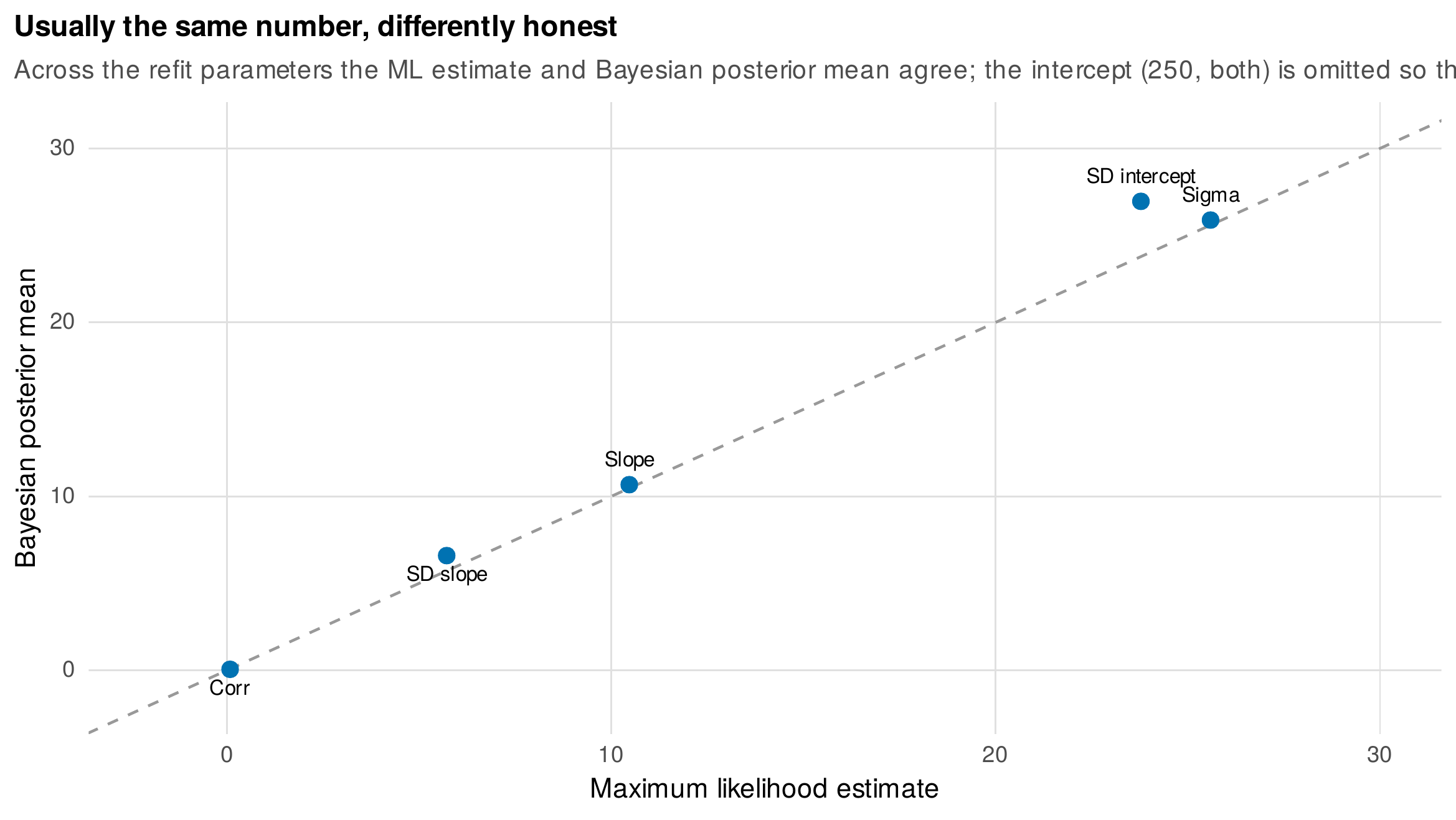
Note. Maximum-likelihood estimates against Bayesian posterior means for the parameters of the sleepstudy model (the intercept, near \(250\) under both, is omitted so the smaller parameters are legible). The estimates lie on the identity line; the random-effect standard deviations are slightly larger under the Bayesian fit, which lacks maximum likelihood’s downward variance bias. Agreement on the numbers, difference in the treatment of uncertainty.
Table 17.4. When to prefer Bayesian estimation or maximum likelihood.
| Prefer Bayesian estimation when | Prefer maximum likelihood when |
|---|---|
| Variances hit boundaries or singular fits | The sample is large and the fit is stable |
| The sample is small and inference must be honest | Speed or convention is paramount |
| Derived quantities need full uncertainty | A quick point estimate suffices |
| The model is weakly identified (scale, dynamic, latent) | The model is standard and well identified |
Note. The book is bilingual. Bayesian estimation earns its cost where maximum likelihood strains, at boundaries, at small samples, and for derived quantities and weakly identified models; maximum likelihood remains the efficient default for large, stable, standard problems.
17.6 Reporting a Bayesian Longitudinal Analysis
A Bayesian analysis is reported to a standard that lets a skeptical reader reconstruct and trust it, and the community has converged on a checklist for the purpose (Depaoli & van de Schoot, 2017). The priors must be stated with their justification, and a prior sensitivity analysis reported, because an unstated prior is an unauditable assumption. The software and its version must be named, since defaults change. The convergence diagnostics, \(\hat{R}\), effective sample size, and the count of divergent transitions, must be reported, not merely asserted to be fine, and any divergences explained or resolved. The posterior is summarized by its central tendency and a credible interval, never by a point estimate alone, and derived quantities are reported with their intervals too. Posterior predictive checks are shown. Table 17.5 is the checklist. A final practical matter is handling the skeptical reviewer or committee: the most effective response is evidence, the agreement plot of Figure 17.10 showing that the Bayesian and frequentist estimates coincide where both are valid, together with a complete reporting of priors and diagnostics that removes the suspicion of hidden choices.
Table 17.5. A reporting checklist for a Bayesian longitudinal analysis.
| Element | What to report |
|---|---|
| Priors | Every prior with its justification, and a sensitivity analysis |
| Software | The package and version, and the sampler settings |
| Convergence | \(\hat{R}\), bulk and tail effective sample size, and divergent transitions |
| Posterior summaries | Central tendency with credible intervals, never a point alone |
| Derived quantities | Reported with their full posterior uncertainty |
| Model checking | Posterior predictive checks and any predictive comparison |
Note. The checklist, adapted from the when-to-worry-about-Bayesian-methods guidance, exists so that a reader can audit every choice. The recurring failure is to report a posterior mean and a credible interval while omitting the priors and the diagnostics that make them trustworthy.
17.7 Running a Bayesian Model in R
The brms package specifies a Bayesian multilevel model in the same formula syntax as lme4 and fits it with Stan, supplying weakly informative default priors that can be inspected and overridden.
library(brms)
# The sleepstudy random-slope model, Bayesian
m <- brm(Reaction ~ Days + (Days | Subject), data = sleepstudy,
         prior = c(prior(normal(0, 50), class = b),          # fixed effects
                   prior(normal(0, 50), class = sd),          # random-effect SDs (half-normal)
                   prior(lkj(2),        class = cor)),        # LKJ on the correlation
         chains = 4, cores = 4, seed = 1)
summary(m)                                                    # posterior summaries + Rhat, ESS
Diagnostics, prior and posterior predictive checks, and predictive comparison are one call each, and derived quantities come from the posterior draws.
pp_check(m)                                    # posterior predictive check
loo(m)                                         # leave-one-out cross-validation
# Prior predictive: refit with sample_prior = "only", then pp_check
# Derived quantity: P(person slope < 0) from the posterior draws
post <- as_draws_df(m)                          # posterior draws, incl. random effects
# Prior sensitivity: refit under 2-3 prior sets and compare posteriors
The complete analysis of this chapter, including the prior predictive and LKJ demonstrations, a transparent Markov chain Monte Carlo sampler with split-\(\hat{R}\) and effective-sample-size functions written from first principles, the funnel geometry, the boundary rescue, the small-sample coverage simulation, and the derived-quantity and agreement displays, is the shipped script ch17_analysis_V01.R, with figures drawn by ch17_figures_V01.R. The script fits the models with its own sampler for transparency and portability; brms with a Stan backend is the recommended production tool, and it is the engine assumed by the later chapters that build on this one.
Software Note • the Bayesian toolchain
Several layers of tool exist. Raw Stan, called through cmdstanr or rstan, offers full control and fits any model that can be written in its language (Carpenter et al., 2017). The brms package writes the Stan program automatically from a formula and is the recommended entry point for the models of this book; rstanarm precompiles a fixed set of models for faster startup at the cost of flexibility. Diagnostics and visualization come from bayesplot and posterior manipulation from the posterior and tidybayes packages, with cross-validation in loo. For the structural-equation models of Part V, blavaan brings the same Stan backend to the latent-variable framework. A caution for cross-program work: Mplus offers a Bayesian estimator whose defaults and diagnostics differ from the Stan ecosystem, reporting a potential scale reduction based on a different construction, a difference that matters when the dynamic structural equation models of Chapter 25 are fit there.
17.8 Common Misconceptions
Several beliefs about Bayesian methods mislead. The first is that Bayesian estimation lets one say anything with small samples; the priors do real work when data are scarce, so a sensitivity analysis is mandatory and a careless prior can harm rather than help (McNeish, 2016). The second is that a credible interval is just a confidence interval with better philosophy; the two are numerically close under weak priors and ample data, but they make different statements, and the difference is exactly what is treated as random. The third is that divergent transitions are warnings to be tolerated; they signal that the sampler could not traverse part of the posterior, so the draws are biased, not merely inefficient, and they must be resolved. The fourth is that cross-validation selects the true model; it estimates predictive accuracy, and the best-predicting model need not be the explanatory one. The fifth is that a flat prior is the objective, assumption-free choice; a flat prior on a variance is a strong and usually implausible statement, as the prior predictive check of Figure 17.2 shows.
Common Pitfall • four errors in Bayesian practice
First, flat priors on variances in the name of objectivity: a flat or very wide prior on a variance implies an extreme prior on the intraclass correlation and other derived quantities; check the implication by prior predictive simulation. Second, ignoring divergences because \(\hat{R}\) looks fine: convergence of the chains does not rule out a region the sampler never reached, so divergences must be addressed on their own, usually by the non-centered parameterization. Third, selecting a model by cross-validation and then interpreting it as the causal truth: predictive ranking is not explanatory warrant. Fourth, reporting a posterior mean of a bounded parameter without its interval: for a variance or a correlation near a boundary the mean alone misleads, and the interval carries the message.
Chapter Summary
Bayesian estimation forms a posterior as the prior times the likelihood and explores it by simulation, and it is the estimation engine that the boundaries, integrals, and latent dynamics of longitudinal modeling repeatedly demand. The posterior yields credible intervals that state the probability a parameter lies in a range, and it is usually data-dominated under weak priors (Figure 17.1). Priors are placed on standard deviations, not variances, using half-normal or half-t densities that permit small variances, and on correlations through the LKJ prior, and every prior is checked by prior predictive simulation because a prior on a variance is a prior on the intraclass correlation and everything else it implies (Figures 17.2 and 17.3, Table 17.1). Markov chain Monte Carlo, with Hamiltonian dynamics, is diagnosed by \(\hat{R}\), effective sample size, and divergent transitions (Figure 17.4, Table 17.2), and the characteristic hierarchical pathology is the funnel, cured not by tuning but by the non-centered reparameterization (Figure 17.5). Models are criticized by posterior predictive checks aimed at the features that matter (Figure 17.6) and compared by cross-validation, which estimates prediction rather than truth (Table 17.3). The payoffs are concrete: a posterior where maximum likelihood gives a boundary point (Figure 17.7), better-calibrated small-sample intervals (Figure 17.8), and full uncertainty on derived quantities (Figure 17.9), all while agreeing with maximum likelihood on the numbers where both are valid (Figure 17.10, Table 17.4). The analysis is reported to an auditable checklist of priors, diagnostics, and checks (Table 17.5).
Where to Go Next
This chapter is consumed by most of what follows. The structural-equation models of Part V, the latent growth and change-score models and the cross-lagged panel models, are increasingly fit by Bayesian estimation through blavaan and the Bayesian options of the commercial programs, and the invariance testing of Chapter 18 gains an approximate, Bayesian form. The intensive-longitudinal models of Part VI depend on it almost entirely: the dynamic structural equation models of Chapter 25 inherit this chapter’s diagnostic table verbatim, and the continuous-time and state-space models of Chapters 26 and 27 are in practice Bayesian. The prediction framing of the cross-validation section returns in Chapter 31, and the reporting checklist feeds the workflow of Chapter 36. The location-scale model of Chapter 16, which sent the reader here for its estimation, can now be refit with the machinery understood rather than borrowed. The habits this chapter instills, checking priors by their implications, reading the diagnostics before the estimates, and propagating uncertainty into every derived quantity, are the working discipline of Bayesian longitudinal analysis.
Exercises
- 17.1 Prior predictive design. For a growth model on an outcome bounded between zero and one hundred, choose priors for the fixed effects and variance components, simulate from them, and show the implied trajectories and intraclass correlation are reasonable before touching the data.
- 17.2 Diagnose and repair. Given three fitted models with planted pathologies, an unmixed chain, a low tail effective sample size, and divergences from a funnel, identify each from its diagnostics and state the repair.
- 17.3 Refit and agree. Refit a mixed model from an earlier chapter under Bayesian estimation, produce the maximum-likelihood-versus-Bayes agreement plot, and account for any parameter where the two differ.
- 17.4 Derived quantities. From the posterior draws, compute the probability that a given person’s slope is negative and a predictive interval for a new person’s trajectory, and write the substantive sentence each supports.
- 17.5 Predictive comparison. Compare a linear and a piecewise growth model by leave-one-out cross-validation, interpret the Pareto-shape flags substantively as influential persons, and state what the comparison does and does not establish.
- 17.6 Prior sensitivity. Refit a model under three defensible prior sets, report the posterior of a key parameter under each, and judge whether the conclusion is robust.
References
Betancourt, M. (2017). A conceptual introduction to Hamiltonian Monte Carlo. arXiv. https://arxiv.org/abs/1701.02434
Bürkner, P.-C. (2017). brms: An R package for Bayesian multilevel models using Stan. Journal of Statistical Software, 80(1), 1–28. https://doi.org/10.18637/jss.v080.i01
Carpenter, B., Gelman, A., Hoffman, M. D., Lee, D., Goodrich, B., Betancourt, M., Brubaker, M., Guo, J., Li, P., & Riddell, A. (2017). Stan: A probabilistic programming language. Journal of Statistical Software, 76(1), 1–32. https://doi.org/10.18637/jss.v076.i01
Depaoli, S., & van de Schoot, R. (2017). Improving transparency and replication in Bayesian statistics: The WAMBS-checklist. Psychological Methods, 22(2), 240–261. https://doi.org/10.1037/met0000065
Gabry, J., Simpson, D., Vehtari, A., Betancourt, M., & Gelman, A. (2019). Visualization in Bayesian workflow. Journal of the Royal Statistical Society: Series A (Statistics in Society), 182(2), 389–402. https://doi.org/10.1111/rssa.12378
Gelman, A. (2006). Prior distributions for variance parameters in hierarchical models. Bayesian Analysis, 1(3), 515–534. https://doi.org/10.1214/06-BA117A
Gelman, A., Carlin, J. B., Stern, H. S., Dunson, D. B., Vehtari, A., & Rubin, D. B. (2013). Bayesian data analysis (3rd ed.). CRC Press. https://doi.org/10.1201/b16018
Kruschke, J. K. (2015). Doing Bayesian data analysis: A tutorial with R, JAGS, and Stan (2nd ed.). Academic Press. https://doi.org/10.1016/C2012-0-00477-2
Lewandowski, D., Kurowicka, D., & Joe, H. (2009). Generating random correlation matrices based on vines and extended onion method. Journal of Multivariate Analysis, 100(9), 1989–2001. https://doi.org/10.1016/j.jmva.2009.04.008
McElreath, R. (2020). Statistical rethinking: A Bayesian course with examples in R and Stan (2nd ed.). CRC Press. https://doi.org/10.1201/9780429029608
McNeish, D. (2016). On using Bayesian methods to address small sample problems. Structural Equation Modeling: A Multidisciplinary Journal, 23(5), 750–773. https://doi.org/10.1080/10705511.2016.1186549
Smid, S. C., McNeish, D., Miočević, M., & van de Schoot, R. (2020). Bayesian versus frequentist estimation for structural equation models in small sample contexts: A systematic review. Structural Equation Modeling: A Multidisciplinary Journal, 27(1), 131–161. https://doi.org/10.1080/10705511.2019.1577140
van de Schoot, R., Depaoli, S., King, R., Kramer, B., Märtens, K., Tadesse, M. G., Vannucci, M., Gelman, A., Veen, D., Willemsen, J., & Yau, C. (2021). Bayesian statistics and modelling. Nature Reviews Methods Primers, 1, Article 1. https://doi.org/10.1038/s43586-020-00001-2
Vehtari, A., Gelman, A., & Gabry, J. (2017). Practical Bayesian model evaluation using leave-one-out cross-validation and WAIC. Statistics and Computing, 27(5), 1413–1432. https://doi.org/10.1007/s11222-016-9696-4
Vehtari, A., Gelman, A., Simpson, D., Carpenter, B., & Bürkner, P.-C. (2021). Rank-normalization, folding, and localization: An improved \(\widehat{R}\) for assessing convergence of MCMC. Bayesian Analysis, 16(2), 667–718. https://doi.org/10.1214/20-BA1221