Chapter 18
Longitudinal Factor Analysis and Measurement Invariance Across Time
The models of the multilevel part treated the outcome as given, a number that means the same thing at every occasion. The structural equation part that opens here questions that assumption, and it opens with measurement for a reason: the framework’s distinctive contribution to the study of change is that it can ask whether an instrument measures the same construct in the same way at every wave, and refuse to compare scores until the answer is yes. This is the check that Chapter 3 wrote and this chapter cashes. If a depression scale’s items function differently at intake and at follow-up, because a symptom has been reinterpreted, a response scale has shifted, or an item has drifted in meaning, then a change in the total score confounds real change in depression with change in measurement, and the elegant growth models of the previous chapters estimate a trajectory of an artifact. Longitudinal measurement invariance is the property that licenses the comparison, and testing for it is neither a preliminary hurdle nor a bureaucratic ritual: a failure of invariance is itself a finding about how a construct is measured and understood over time. This chapter specifies the longitudinal factor model, executes the invariance-testing sequence with the exact bookkeeping the reader must master, handles the common case in which invariance partially fails, extends the machinery to categorical items, and demonstrates by simulation what ignoring the whole question costs.
Learning Objectives
After working through this chapter, you should be able to: (1) specify a longitudinal confirmatory factor model with correlated uniquenesses and defend that specification; (2) execute the configural, metric, scalar, and strict invariance sequence with correct identification at each step; (3) adjudicate invariance with fit-difference criteria while knowing their limits; (4) locate noninvariant parameters and implement a defensible partial invariance; (5) run invariance testing with categorical indicators; (6) explain by simulation how ignored noninvariance biases estimates of change; and (7) report an invariance analysis to a complete standard.
18.1 The Longitudinal Measurement Model
A construct measured by several items at several occasions is represented by a longitudinal confirmatory factor model: one latent factor per occasion, each measured by the same set of indicators, with the factors free to covary across time. Figure 18.1 draws the structure for two occasions, and it generalizes to any number. The essential feature that distinguishes the longitudinal model from a stack of separate cross-sectional factor models is the treatment of the uniquenesses, the indicator residuals. The same item measured at two occasions shares more than the common factor: it carries an indicator-specific component, a stable idiosyncrasy of that particular question that persists across time and has nothing to do with the construct. A vocabulary item may be reliably easy for reasons unrelated to verbal ability; a survey item may be consistently read in a particular way. This shared indicator-specific variance induces a correlation between the same item’s residuals across waves, and the longitudinal factor model must include these correlated uniquenesses. Omitting them does not merely lose a nuisance parameter; it forces the indicator-specific stability to be absorbed into the only pathway left for it, the correlation among the factors, and so inflates the estimated stability of the construct itself.
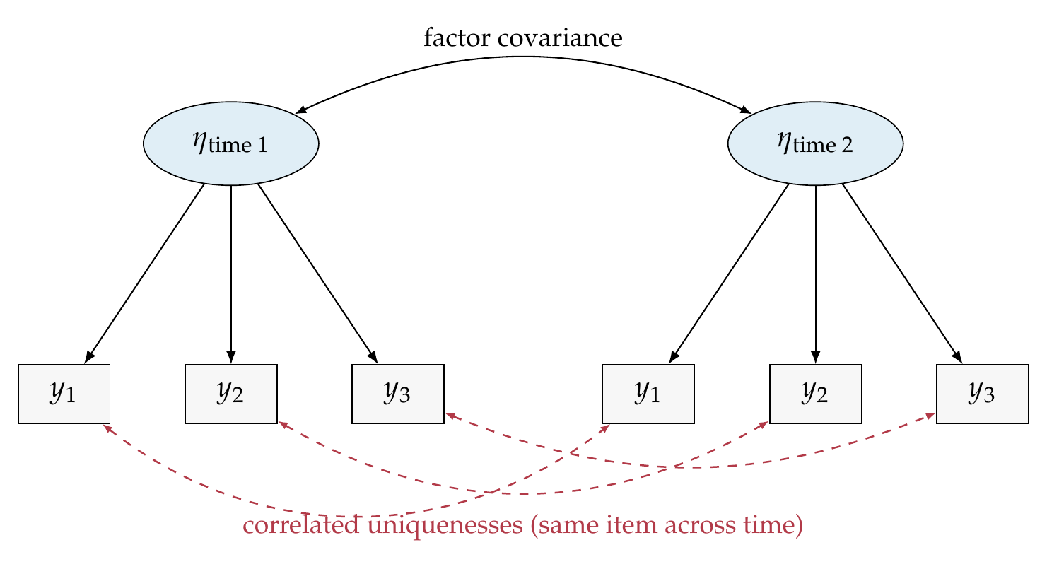
Note. One factor per occasion, each measured by the same indicators, with the factors free to covary. The dashed arrows are the correlated uniquenesses that link each indicator’s residual to itself across time, capturing indicator-specific stable variance. Omitting them forces that stability into the factor covariance and inflates the apparent stability of the construct. The diagram generalizes to any number of waves.
The bias is not hypothetical, and Figure 18.2 quantifies it on the running dataset, a simulated four-wave, three-indicator engagement scale with a known measurement model. When the correlated uniquenesses are included, the estimated factor correlations track their true values; when they are omitted, every factor correlation is inflated, so that a researcher would overstate how much a person’s standing on the construct at one wave predicts their standing at the next. Correlated uniquenesses are therefore the default backbone of a longitudinal factor model, not an optional refinement.
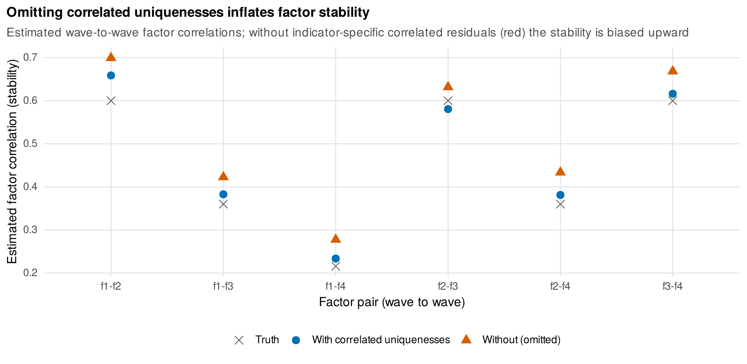
Note. Estimated wave-to-wave factor correlations from the engagement data, with and without correlated uniquenesses, against their true values. Omitting the correlated residuals (red) pushes every factor correlation upward, overstating the stability of the construct. The indicator-specific stable variance has nowhere else to go.
Before the factors can be compared across time, the model must be identified, and identification in a mean-and-covariance-structure model is a system of bookkeeping that trips many users. The latent variables have no inherent scale or origin, so each factor needs a scale and a zero point fixed by convention, and there are three conventions in use: the marker-variable method fixes one loading to one and its intercept to zero; the fixed-factor method fixes the factor variance to one and the factor mean to zero; and the effects-coding method constrains the loadings to average one and the intercepts to sum to zero. The conventions interact with the invariance constraints, because what a given constraint identifies depends on what has already been fixed, and Table 18.1 lays out the grid. The practical rule is to choose one convention, apply it consistently, and account for every degree of freedom at every step, which is the discipline this chapter models throughout. Fit is evaluated with the indices of Chapter 8, the comparative fit index, the root mean square error of approximation, and the standardized root mean square residual, read against their conventional benchmarks with the standing caution that those benchmarks are rules of thumb from particular simulation conditions, not laws, and are used here as diagnostics rather than verdicts.
Table 18.1. Scaling conventions and what each invariance step constrains.
| Convention | Scale set by | Consequence for invariance testing |
|---|---|---|
| Marker variable | One loading \(=1\), its intercept \(=0\) | The marker is assumed invariant; other loadings and intercepts are tested |
| Fixed factor | Factor variance \(=1\), mean \(=0\) | Frees all loadings to be tested; the variance must be freed at later waves once metric holds |
| Effects coding | Loadings average \(1\), intercepts sum to \(0\) | Keeps the factor in the indicators’ metric; distributes the identification across items |
Note. The three conventions give identical fit and identical substantive conclusions, but they place the identifying constraints differently, so the degrees of freedom freed and constrained at each invariance step differ. Choose one and apply it consistently; the marker method is used in this chapter’s worked example.
18.2 The Invariance Ladder
Measurement invariance is tested as a sequence of nested models, each adding a set of equality constraints across time and each licensing a further kind of comparison. Figure 18.3 shows the sequence run on the engagement scale, and the pattern is the object of study. Configural invariance requires only that the same factor structure, the same items loading on the same factor, holds at every occasion; it establishes that the construct has the same form over time but licenses no quantitative comparison. Metric (or weak) invariance adds equality of the factor loadings across time, and it is what licenses comparing covariances and regression slopes involving the factor, because equal loadings mean a unit of the factor has the same meaning at every wave. Scalar (or strong) invariance adds equality of the indicator intercepts, and it is the crucial level for the study of change, because only when both loadings and intercepts are invariant can the factor means be compared across time, which is to say only then does a change in the latent mean reflect change in the construct rather than drift in the measurement. Strict invariance adds equality of the indicator residual variances, which licenses the comparison of observed composite scores, since only then do equal factor standings imply equal expected observed scores. Table 18.2 states what each level constrains, means, and licenses.
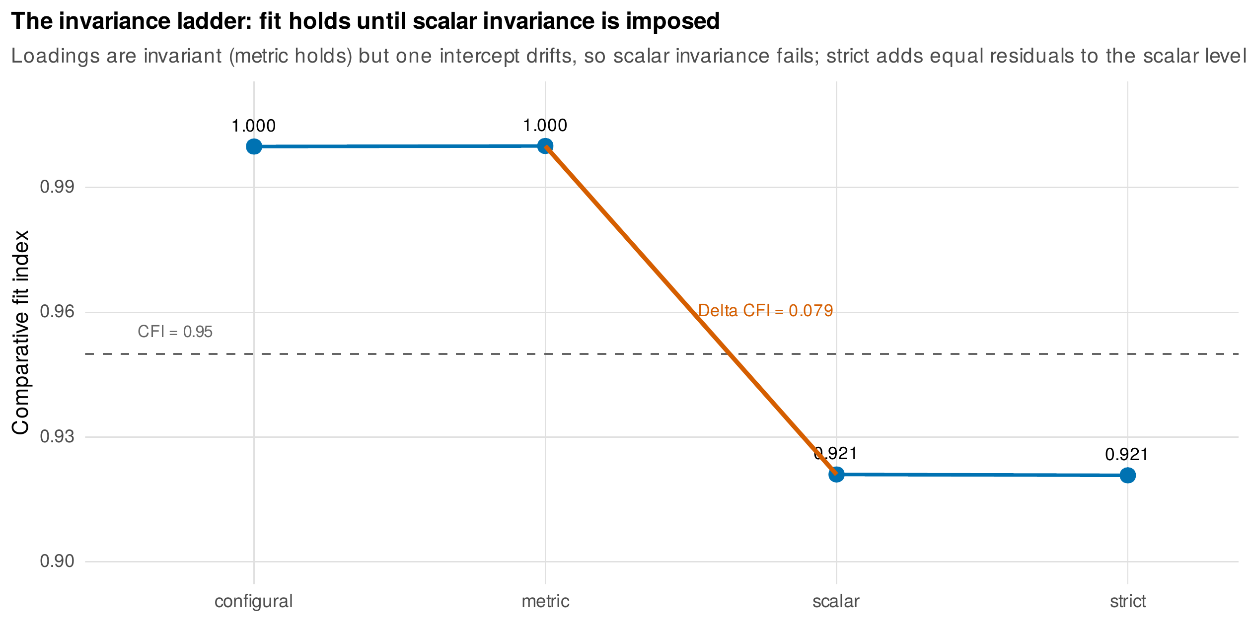
Note. Comparative fit index across the four nested invariance models on the engagement scale. Configural and metric invariance fit well, so the loadings are invariant, but imposing scalar invariance, equal intercepts, collapses the fit, because one indicator’s intercept drifts. Strict invariance adds equal residuals to the already-failing scalar level. The change in fit at the scalar step, not its absolute value, carries the message.
On the engagement data the sequence tells a clear story. The configural model fits well, with a comparative fit index of \(1.00\) and a root mean square error of approximation of \(.006\). Metric invariance holds: constraining the loadings equal across the four waves changes the chi-square by only \(1.9\) on six degrees of freedom, far from significant, and leaves the fit indices unchanged. Scalar invariance fails decisively: constraining the intercepts equal worsens the chi-square by \(374\) on six degrees of freedom and drops the comparative fit index by \(.079\), from \(1.00\) to \(.92\). The story is that the items load on the construct identically over time, so the construct has the same meaning, but at least one item’s intercept has drifted, so the observed scores are not on a common footing and the latent means cannot yet be compared. Adjudicating this requires decision criteria, and the chapter’s policy, following the reporting literature, is to report several. The chi-square difference test is exact but sensitive to sample size, flagging trivial noninvariance in large samples; the change in the comparative fit index, with a heuristic threshold near \(.01\), and the change in the root mean square error of approximation are less sample-dependent but were calibrated for multi-group rather than longitudinal comparisons, a transfer that should be noted; and an effect-size measure of the magnitude of noninvariance completes the picture. Table 18.3 collects the criteria with their cautions. Here every criterion agrees, because the planted violation is large, but the honest analyst reports the set and does not lean on a single cutoff.
Table 18.2. The invariance ladder: constraints, meaning, and licensed comparisons.
| Level | Constrains across time | Licenses |
|---|---|---|
| Configural | Same factor pattern | The construct has the same form; no quantitative comparison |
| Metric | Loadings | Comparison of covariances and regression slopes |
| Scalar | Loadings and intercepts | Comparison of latent means (change) |
| Strict | Loadings, intercepts, residuals | Comparison of observed composite scores |
Note. Each level adds constraints and licenses a further comparison. The study of latent change requires scalar invariance, because only equal loadings and intercepts make a change in the factor mean a statement about the construct rather than the measurement. Composite scores silently assume the strict level.
Foundations Box • Meredith’s formalization and the selection theorem
The invariance ladder is not an arbitrary sequence of convenience but follows from a formal definition. Meredith (1993) defined measurement invariance through the conditional distribution of the observed indicators given the true construct: measurement is invariant when that conditional distribution is the same across occasions or groups, so that two people with the same construct value have the same expected item responses regardless of when or where they are measured. Weak invariance constrains the loadings, strong invariance adds the intercepts, and strict invariance adds the residual variances, matching the metric, scalar, and strict levels above. The definition is tied to a selection theorem: if a population is selected on variables related to the construct, factorial invariance is preserved under the selection precisely when the measurement parameters are invariant, which is why invariance is the property that makes comparisons across selected or evolving populations, including the same people at different ages, legitimate. The formalization matters because it shows that the constraints test a coherent hypothesis about the measurement process, not merely the fit of successive models.
Table 18.3. Criteria for adjudicating an invariance step.
| Criterion | Heuristic | Caution |
|---|---|---|
| Chi-square difference | Significance at the step | Sensitive to sample size; flags trivial noninvariance when \(N\) is large |
| Change in comparative fit index | Worsening beyond about \(.01\) | Calibrated for multi-group, not longitudinal, comparisons |
| Change in RMSEA | Worsening beyond about \(.015\) | Same transfer caveat; less sample-dependent |
| Effect size of noninvariance | Magnitude of the difference | Distinguishes detectable from consequential |
Note. No single criterion is decisive. The book’s policy is to report the set together with an effect-size measure of the magnitude of noninvariance, so that a statistically detectable but practically negligible difference is not mistaken for a consequential one, and vice versa.
18.3 When Invariance Fails
A failure of scalar invariance is the beginning of the analysis, not its end. The first task is to locate the noninvariant parameter. Because a model with equality constraints hides the offending parameter from the ordinary modification index, which is computed for a single model, the forensic tool is the score test that evaluates releasing each constraint, or equivalently the transparent procedure of refitting the model while freeing one indicator’s intercepts at a time and seeing which restores fit. Figure 18.4 shows the result: freeing the second indicator’s intercepts returns the comparative fit index to \(1.00\), while freeing either other indicator does not, identifying the second item as the culprit. The location should be interrogated with theory rather than chased greedily, because releasing constraints purely to improve fit capitalizes on chance and can free parameters that are noninvariant only by sampling noise. Figure 18.5 shows the anatomy of the violation directly: the second indicator, which has the smallest loading, nonetheless shows the largest change from the first wave at waves three and four, a pattern impossible under invariance, where an item’s change should be proportional to its loading times the factor’s change. The item has drifted upward in its baseline, contributing more to the observed score at later waves than the construct warrants.
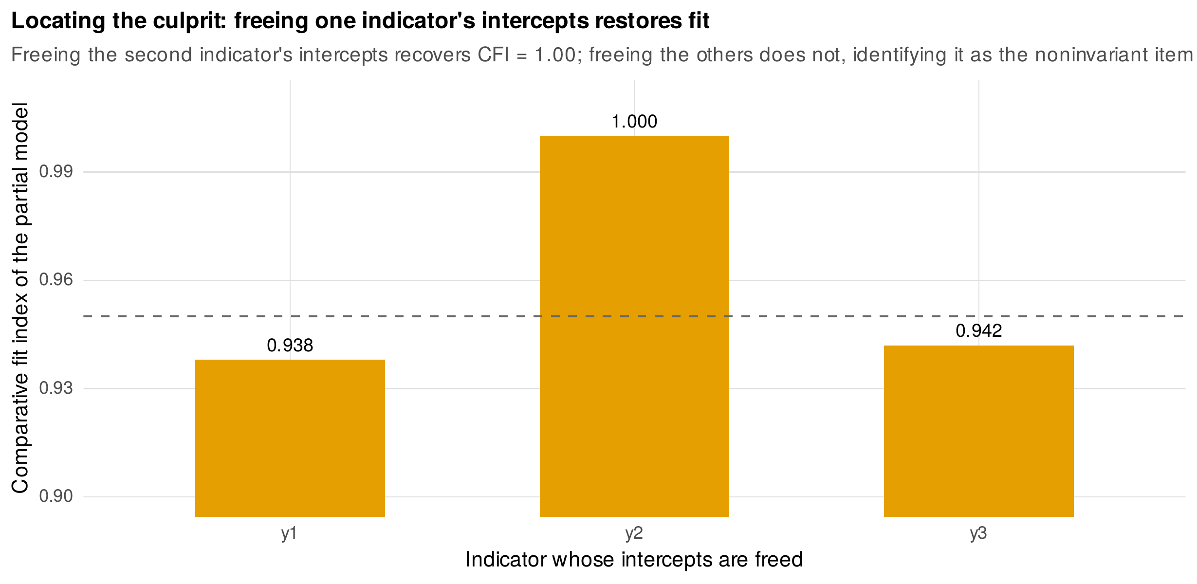
Note. Comparative fit index of the scalar model when each indicator’s intercepts are freed across waves. Freeing the second indicator restores fit to \(1.00\); freeing either other indicator leaves the model misfitting. This identifies the second item as the noninvariant one, the forensic use of the score test rather than a greedy search.
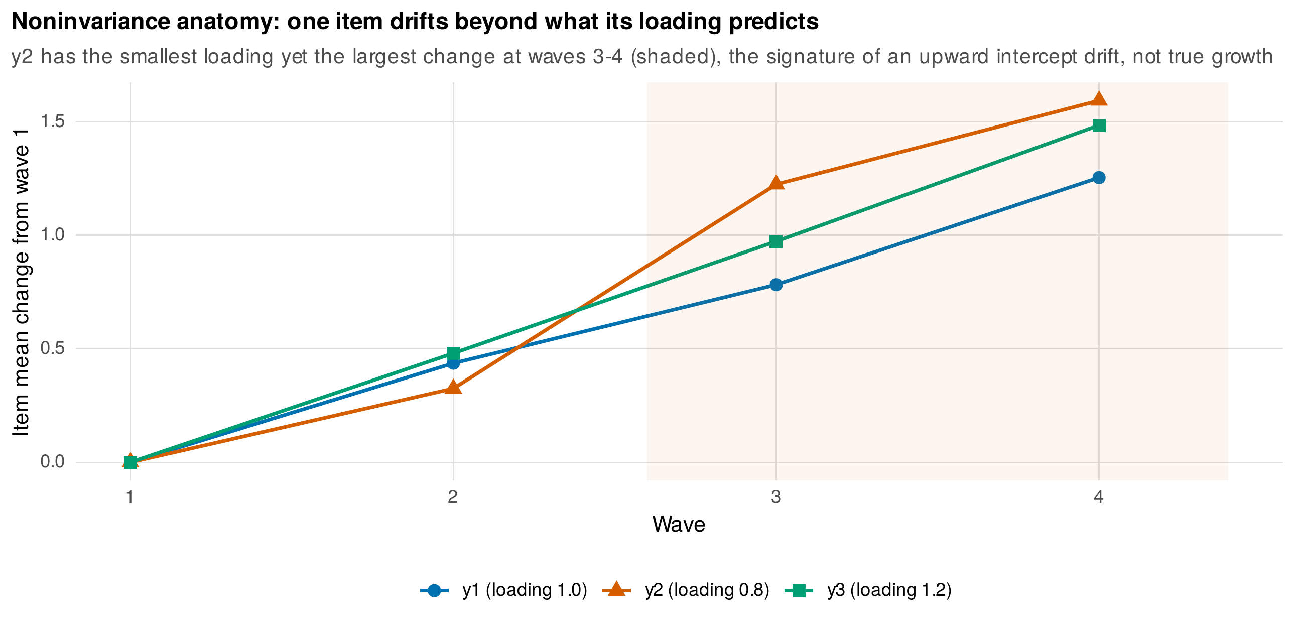
Note. Mean change from the first wave for each indicator. Under invariance an item’s change equals its loading times the factor’s change, so the highest-loading item should change most. Instead the second item, with the smallest loading, changes most at waves three and four (shaded), the signature of an upward intercept drift rather than true growth.
Having located the violation, the analyst adopts partial invariance, freeing the offending intercept while holding the others equal, an approach introduced by Byrne, Shavelson, and Muthén (1989). Freeing the second indicator’s intercepts at waves three and four restores the fit to a comparative fit index of \(1.00\), and the latent means can now be compared, resting on the invariant remainder of the scale as anchor items. The honest questions are how much partiality is too much and which items may serve as anchors, and they have no mechanical answer: a scale on which most items have drifted cannot support a credible comparison, and the defensible practice is to keep a substantial majority of items invariant, to justify the anchor set on substantive grounds, and to report a sensitivity analysis showing that the conclusions hold under alternative choices of which items to free. Crucially, the noninvariance is itself a substantive finding. An item that drifts has changed its relationship to the construct, which may reflect recalibration by respondents, a shift in what the item measures, or a genuine change in the construct’s manifestation, the heterotypic continuity of Chapter 3, and in clinical contexts it connects to the response-shift literature on how patients reinterpret a scale as their condition evolves. When full invariance is untenable, more flexible alternatives exist, including approximate invariance through Bayesian small-variance priors that allow measurement parameters to differ slightly rather than exactly, and the alignment method that optimizes a compromise across many groups or occasions (Asparouhov & Muthén, 2014), though their guidance for longitudinal use is still developing.
18.4 Categorical Indicators
Psychological items are often ordinal, a handful of ordered response categories rather than a continuous scale, and invariance testing must then work on the latent response distribution underlying the categories. Each ordinal item is modeled as a coarsening of a latent continuous response by a set of thresholds, and Figure 18.6 draws the idea: a five-category item arises from four thresholds carving a latent normal response into ordered bands. Invariance for categorical items therefore concerns the thresholds as well as the loadings, and the two are coupled in a way that requires a specific testing sequence and specific identification constraints, worked out by Wu and Estabrook (2016) and adapted to the longitudinal case by Liu and colleagues (2017). Estimation is typically by a weighted least squares method, robust to the non-normality of ordinal data, rather than maximum likelihood. Table 18.4 contrasts the continuous and categorical procedures. A practical consideration links back to Chapter 6: the weighted least squares estimator handles missing data less gracefully than the full-information maximum likelihood of the continuous model, using a pairwise-style treatment that assumes a more restrictive missingness mechanism, so with substantial missingness a maximum-likelihood approach with a robust correction, or a fully Bayesian treatment, may be preferable. On the engagement items recoded to five categories, the configural and threshold-and-loading-invariant models both fit, illustrating the machinery; the full categorical sequence, with its careful identification, is developed in the references.
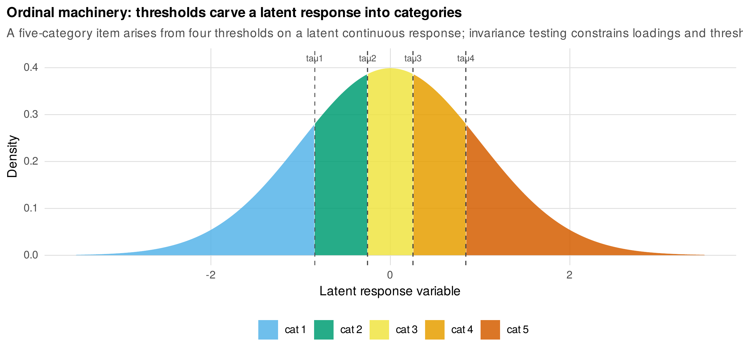
Note. A five-category ordinal item is modeled as a latent continuous response variable coarsened by four thresholds. Invariance testing for categorical items constrains the loadings and the thresholds together, on the latent response scale, and is estimated by robust weighted least squares rather than maximum likelihood.
Table 18.4. Continuous and categorical invariance procedures compared.
| Feature | Continuous indicators | Categorical indicators |
|---|---|---|
| Tested parameters | Loadings, intercepts, residuals | Loadings, thresholds, residuals |
| Estimator | Maximum likelihood | Robust weighted least squares |
| Scaling | Marker, fixed-factor, or effects coding | Plus delta or theta parameterization |
| Missing data | Full-information maximum likelihood | Pairwise-style; more restrictive |
Note. Categorical invariance replaces the intercepts with thresholds on the latent response and couples them to the loadings, requiring a specific sequence and identification (Wu & Estabrook, 2016; Liu et al., 2017). The estimator’s weaker missing-data handling is a reason to prefer maximum likelihood with robust corrections when missingness is substantial.
18.5 Why This Labor Matters
The motivation for the entire apparatus is that ignoring noninvariance biases the study of change, and a simulation makes the cost concrete. Figure 18.7 shows the recovered latent-mean trajectory of the engagement construct under three analytic choices, against the known truth. The truth is a steady growth of \(0.4\) per wave. The composite score, the average of the items, which silently assumes strict invariance, overstates the later growth, because the drifting item inflates the composite at waves three and four. A factor model that wrongly imposes full scalar invariance does the same, attributing the item’s drift to the factor mean. Only the partial-invariance model, which frees the drifting intercept, recovers the true trajectory. The bias is not a rounding error: at the final wave the composite estimates a change of \(1.44\) against the true \(1.20\), a twenty-percent overstatement of the construct’s growth, and Figure 18.8 shows that the overstatement grows without bound as the drift increases, while the partial-invariance estimate stays near the truth regardless. This simulation is the argument for the measurement-first sequence of the structural equation part: a growth model, however sophisticated, inherits the biases of the scores it is fit to, and the second-order growth model of Chapter 20, which fits the trajectory to the invariant latent factors rather than to the composites, is the proper remedy. Factor scores extracted from an invariance analysis and then fed into a growth model are a tempting shortcut but carry their own hazards, because the scores are estimated with error that the second stage ignores, a plug-in problem best avoided by fitting the measurement and growth models jointly.
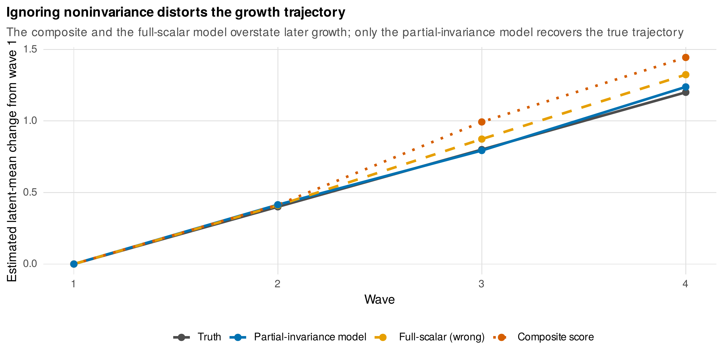
Note. Recovered latent-mean change of the engagement construct under three analytic choices, against the known truth. The composite score and the wrongly-full-scalar factor model overstate the later growth, because the drifting item inflates them; only the partial-invariance model recovers the true trajectory. This is the argument for measurement-first analysis of change.
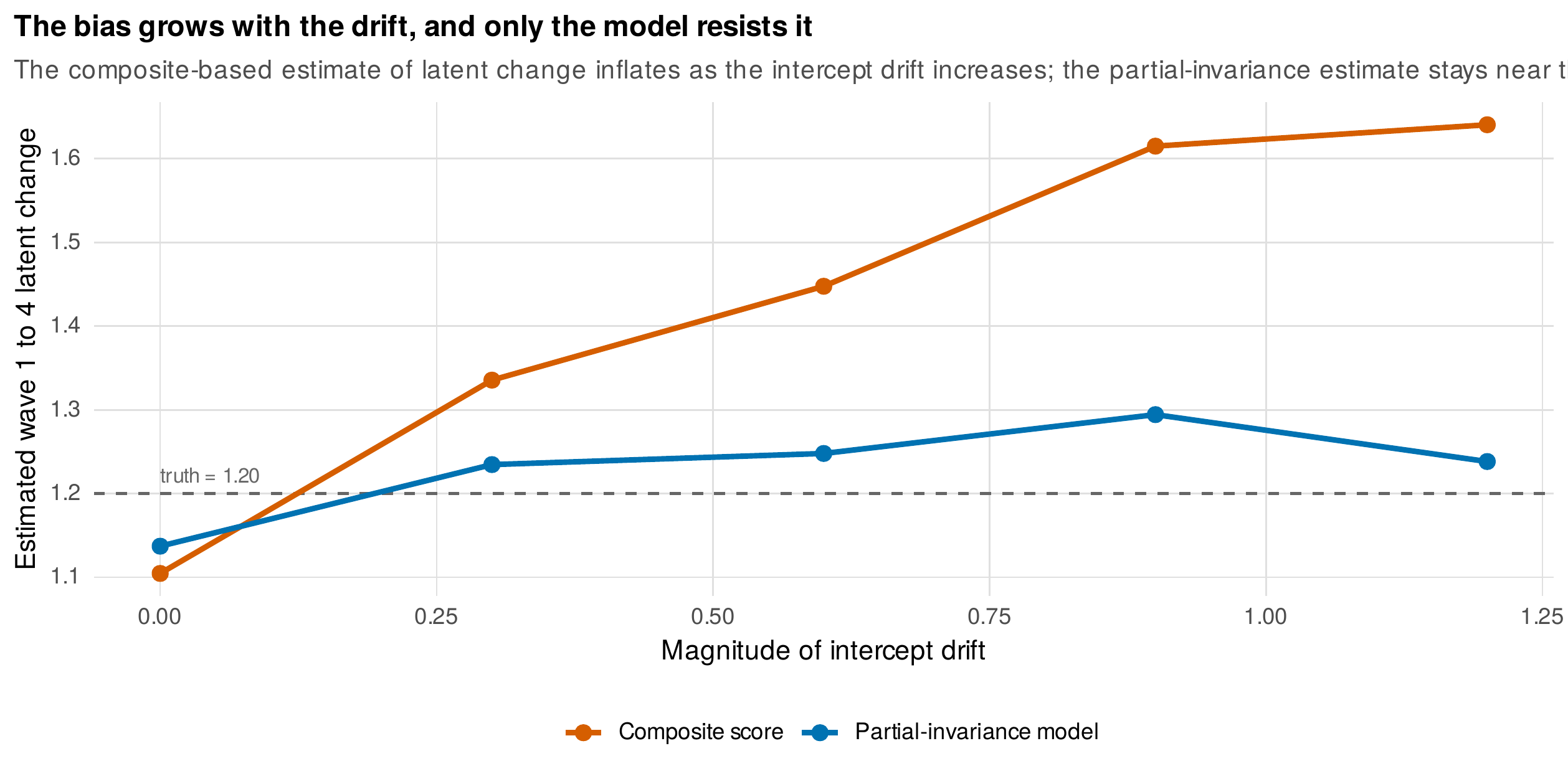
Note. The estimated wave-one-to-wave-four latent change against the magnitude of the intercept drift, for the composite score and the partial-invariance model. The composite’s estimate inflates as the drift grows; the partial-invariance model’s estimate stays near the truth. Noninvariance is not self-correcting, and larger drift means larger bias.
18.6 Reporting an Invariance Analysis
An invariance analysis is reported so that a reader can follow every constraint and reproduce every decision, and the field has documented how uneven this reporting has been (Putnick & Bornstein, 2016). The report states the longitudinal factor model, including the correlated uniquenesses and the scaling convention; presents the sequence of models as a table with the fit of each and the fit difference at each step under the several criteria; names any noninvariant parameters and the evidence locating them; states the partial-invariance decisions and the anchor logic; and reports a sensitivity analysis showing that the substantive conclusions survive alternative partial specifications. Table 18.5 is the checklist and the template for the sequence table that every such paper needs. The write-up interprets noninvariance substantively where it occurs rather than burying it as a technical caveat, because a drifting item is a finding about the construct.
Table 18.5. A reporting checklist and sequence-table template for invariance.
| Element | What to report |
|---|---|
| Measurement model | The factors, indicators, correlated uniquenesses, and scaling convention |
| The sequence table | Each model with its fit indices and the fit difference at each step |
| Decision criteria | The chi-square difference, the change in fit indices, and an effect size |
| Noninvariant parameters | Which parameters were freed and the evidence locating them |
| Partial-invariance logic | The anchor items and the justification for the freed set |
| Sensitivity | Conclusions under alternative partial specifications |
Note. The sequence table, with a row per model and columns for the fit indices and their differences, is the exhibit every invariance paper needs. Noninvariance is reported and interpreted substantively, not hidden, because item drift is a finding.
18.7 Running the Invariance Sequence in R
The longitudinal factor model and the invariance constraints are specified in lavaan by labeling the parameters that are to be held equal across waves. The correlated uniquenesses are added as residual covariances between each indicator and itself across time.
library(lavaan)
config <- '
  f1 =~ 1*y1w1 + L2_1*y2w1 + L3_1*y3w1     # loadings free per wave (configural)
  f2 =~ 1*y1w2 + L2_2*y2w2 + L3_2*y3w2
  f3 =~ 1*y1w3 + L2_3*y2w3 + L3_3*y3w3
  f4 =~ 1*y1w4 + L2_4*y2w4 + L3_4*y3w4
  y1w1 ~~ y1w2 + y1w3 + y1w4                # correlated uniquenesses ...
  y2w1 ~~ y2w2 + y2w3 + y2w4                # ... same indicator across waves
  y3w1 ~~ y3w2 + y3w3 + y3w4  '
m_config <- sem(config, data = engage_long, meanstructure = TRUE)
Metric invariance gives the loadings a shared label across waves (L2, L3); scalar invariance additionally shares the intercept labels and frees the latent means; strict invariance additionally shares the residual labels. Adjacent models are compared with anova and their fit with fitMeasures.
anova(m_config, m_metric, m_scalar, m_strict)          # nested chi-square tests
fitMeasures(m_scalar, c("cfi","rmsea","srmr"))          # fit of each level
# Locate a violation by freeing one indicator's intercepts and refitting,
# or with lavTestScore(m_scalar) for the score tests on the equality constraints.
# Ordinal items: sem(..., ordered = c("oy1w1", ...), estimator = "WLSMV")
The complete analysis, including the correlated-uniqueness bias demonstration, the full ladder with degree-of-freedom accounting, the location and partial-invariance repair, the latent-mean recovery, the consequences simulation, and the ordinal fit, is the shipped script ch18_analysis_V01.R, with figures drawn by ch18_figures_V01.R and the dataset generated by gen_engage_long_V01.R. The analysis writes the equality constraints explicitly for transparency; in practice the semTools package automates the entire sequence.
Software Note • tools for invariance testing
The semTools package builds the longitudinal invariance models automatically through its measEq.syntax function, which generates the labeled lavaan syntax for each level under any scaling convention and handles the categorical case with the correct thresholds and parameterization, so that in practice one does not hand-write the constraints; the explicit syntax of this chapter is for understanding what that function produces. In Mplus the sequence is requested through the MODEL = CONFIGURAL METRIC SCALAR convenience option, and the robust chi-square difference for categorical models through DIFFTEST. The blavaan package fits the same models by the Bayesian estimation of Chapter 17, which is the route to approximate invariance through small-variance priors on the measurement-parameter differences, a Bayesian relaxation of the exact-equality constraints tested here.
18.8 Common Misconceptions
Several beliefs about invariance mislead. The first is that invariance is a preliminary hurdle rather than science; a failure of invariance is a substantive finding about how a construct is measured and understood over time, and item drift can be the most interesting result in a study. The second is that the chi-square difference test is too sensitive and should be ignored entirely; it is sensitive to sample size, which is a reason to report it alongside effect sizes and fit-difference indices, not to discard it. The third is a pair of opposite errors, that freeing a single loading invalidates the whole analysis and that one should free whatever the modification indices suggest; the truth is that partial invariance with a well-justified minority of freed parameters supports valid comparison, while greedy freeing capitalizes on chance. The fourth is that composite scores sidestep the invariance question; they do not, they silently assume the strict level, and the consequences simulation shows the cost when that assumption is false. The fifth is that latent means can be compared once the model fits; they can be compared only once scalar invariance, at least partial, is established.
Common Pitfall • four errors in invariance practice
First, omitting correlated uniquenesses: without them the indicator-specific stability inflates the factor correlations and the apparent stability of the construct (Figure 18.2). Second, comparing latent means without scalar invariance: a mean difference then confounds construct change with intercept drift. Third, chasing modification indices greedily: free parameters on substantive grounds with a sensitivity analysis, not to maximize fit. Fourth, treating a fit-index cutoff as a law: the change-in-fit thresholds were calibrated for particular conditions and are diagnostics, not verdicts; report several criteria.
Chapter Summary
Longitudinal measurement invariance is the property that licenses comparing a construct across time, and testing it is the measurement foundation of the structural equation approach to change. The longitudinal factor model places one factor per occasion, measured by the same indicators, with correlated uniquenesses that capture indicator-specific stability and whose omission inflates the estimated stability of the construct (Figures 18.1 and 18.2). Identification follows one of three scaling conventions, applied consistently with full degree-of-freedom bookkeeping (Table 18.1). The invariance ladder, configural, metric, scalar, strict, adds constraints that license successively covariance comparison, mean comparison, and composite comparison (Figure 18.3, Table 18.2), and follows from Meredith’s formalization; the steps are adjudicated by several criteria, none decisive alone (Table 18.3). When invariance fails, the violation is located forensically and repaired by partial invariance with justified anchors (Figures 18.4 and 18.5), and the drift is interpreted as a finding. Categorical items are tested on their thresholds by robust weighted least squares (Figure 18.6, Table 18.4). The labor matters because ignoring noninvariance biases the trajectory of change, as the composite and the wrongly-invariant model overstate growth while the partial-invariance model recovers the truth (Figures 18.7 and 18.8), the argument for the measurement-first, second-order approach of the chapters to come. The analysis is reported to a complete sequence-table standard (Table 18.5).
Where to Go Next
This chapter is the measurement foundation on which the rest of the structural equation part builds. Chapter 19 fits the latent growth curve model, revealing it to be the same growth model as Chapter 14 in structural-equation form, and Chapter 20 develops the second-order growth model that fits the trajectory to the invariant latent factors of this chapter rather than to composite scores, the proper remedy for the bias demonstrated here. Chapter 21 makes the invariance assumptions inside the cross-lagged panel models explicit, and Chapter 22 extends the question to invariance across latent classes. In the intensive-longitudinal part, Chapter 25 confronts the within-person factor structure that dynamic models assume. The vertical-scaling problems of large-scale assessment in Chapter 34 are invariance problems in another guise. The discipline this chapter models, accounting for every constraint and every degree of freedom, and interpreting a failure of invariance as a finding rather than a nuisance, is the working habit of measurement-conscious longitudinal research.
Exercises
- 18.1 Specify and count. Write the syntax for a three-indicator, four-wave longitudinal factor model under two scaling conventions, and produce the degree-of-freedom accounting for the configural through strict models.
- 18.2 Run the ladder. On a dataset with a planted noninvariant intercept, run the full sequence, locate the violation, free it with justification, and report the sequence table.
- 18.3 Ordinal invariance. Fit configural and threshold-invariant models to ordinal items with a robust weighted least squares estimator, and interpret the comparison.
- 18.4 Extend the consequences. Vary the magnitude of the intercept drift and plot the resulting bias in the estimated latent change, reproducing the slope-bias curve.
- 18.5 Write the section. From provided output, write the measurement-and-results text for an invariance analysis, interpreting the noninvariance substantively.
References
Asparouhov, T., & Muthén, B. (2014). Multiple-group factor analysis alignment. Structural Equation Modeling: A Multidisciplinary Journal, 21(4), 495–508. https://doi.org/10.1080/10705511.2014.919210
Byrne, B. M., Shavelson, R. J., & Muthén, B. (1989). Testing for the equivalence of factor covariance and mean structures: The issue of partial measurement invariance. Psychological Bulletin, 105(3), 456–466. https://doi.org/10.1037/0033-2909.105.3.456
Chen, F. F. (2007). Sensitivity of goodness of fit indexes to lack of measurement invariance. Structural Equation Modeling: A Multidisciplinary Journal, 14(3), 464–504. https://doi.org/10.1080/10705510701301834
Cheung, G. W., & Rensvold, R. B. (2002). Evaluating goodness-of-fit indexes for testing measurement invariance. Structural Equation Modeling: A Multidisciplinary Journal, 9(2), 233–255. https://doi.org/10.1207/S15328007SEM0902_5
Little, T. D. (2013). Longitudinal structural equation modeling. Guilford Press.
Liu, Y., Millsap, R. E., West, S. G., Tein, J.-Y., Tanaka, R., & Grimm, K. J. (2017). Testing measurement invariance in longitudinal data with ordered-categorical measures. Psychological Methods, 22(3), 486–506. https://doi.org/10.1037/met0000075
Meredith, W. (1993). Measurement invariance, factor analysis and factorial invariance. Psychometrika, 58(4), 525–543. https://doi.org/10.1007/BF02294825
Millsap, R. E. (2011). Statistical approaches to measurement invariance. Routledge. https://doi.org/10.4324/9780203821961
Nye, C. D., & Drasgow, F. (2011). Effect size indices for analyses of measurement equivalence: Understanding the practical importance of differences between groups. Journal of Applied Psychology, 96(5), 966–980. https://doi.org/10.1037/a0022955
Putnick, D. L., & Bornstein, M. H. (2016). Measurement invariance conventions and reporting: The state of the art and future directions for psychological research. Developmental Review, 41, 71–90. https://doi.org/10.1016/j.dr.2016.06.004
Rosseel, Y. (2012). lavaan: An R package for structural equation modeling. Journal of Statistical Software, 48(2), 1–36. https://doi.org/10.18637/jss.v048.i02
Vandenberg, R. J., & Lance, C. E. (2000). A review and synthesis of the measurement invariance literature: Suggestions, practices, and recommendations for organizational research. Organizational Research Methods, 3(1), 4–70. https://doi.org/10.1177/109442810031002
van de Schoot, R., Lugtig, P., & Hox, J. (2012). A checklist for testing measurement invariance. European Journal of Developmental Psychology, 9(4), 486–492. https://doi.org/10.1080/17405629.2012.686740
Widaman, K. F., Ferrer, E., & Conger, R. D. (2010). Factorial invariance within longitudinal structural equation models: Measuring the same construct across time. Child Development Perspectives, 4(1), 10–18. https://doi.org/10.1111/j.1750-8606.2009.00110.x
Widaman, K. F., & Reise, S. P. (1997). Exploring the measurement invariance of psychological instruments: Applications in the substance use domain. In K. J. Bryant, M. Windle, & S. G. West (Eds.), The science of prevention: Methodological advances from alcohol and substance abuse research (pp. 281–324). American Psychological Association.
Wu, H., & Estabrook, R. (2016). Identification of confirmatory factor analysis models of different levels of invariance for ordered categorical outcomes. Psychometrika, 81(4), 1014–1045. https://doi.org/10.1007/s11336-016-9506-0