Chapter 19
Latent Growth Curve Models
Chapter 14 modeled growth as a multilevel model, with person-specific intercepts and slopes drawn from a distribution. This chapter models the same growth as a structural equation model, with the intercept and slope reconceived as latent factors that the repeated measurements load on. The two are, under matched assumptions, the identical model, and this chapter is written in deliberate lockstep with Chapter 14, on the same data and with the same coding decisions, so that their equivalence is something the reader verifies rather than accepts on faith. The point is not that one framework is better. It is that they are two dialects of one language, and a researcher fluent in both can choose the one whose ergonomics fit the question. The structural equation dialect brings its own gifts: it thinks natively in mean structures and global fit, it lets the growth factors serve as predictors and outcomes inside larger systems of variables, it fits multiple groups and multiple parallel processes with ease, and it estimates the shape of change directly through freed loadings. The multilevel dialect brings others, chiefly its effortless handling of individually varying measurement times. The equivalence and its exceptions are the intellectual center of the chapter, and everything else, the conditional models, the multiple-group comparisons, the parallel processes, follows from seeing growth as constraints on the means and covariances of the repeated measures.
Learning Objectives
After working through this chapter, you should be able to: (1) specify a linear latent growth curve model with its mean structure and interpret the intercept and slope factor means, variances, and covariance; (2) state the identification requirements by number of waves and growth form; (3) translate a multilevel growth model into a latent curve model and back, and enumerate the conditions under which they are equivalent and the points at which they diverge; (4) evaluate the fit of a growth model and locate misfit in the mean structure; (5) add covariates and distal outcomes to a conditional growth model; (6) fit a multiple-group growth model with a constraint-testing sequence; (7) fit a parallel-process model and interpret its slope-slope association with due caution; and (8) estimate a nonlinear shape through freed loadings.
19.1 The Model, From the Path Diagram Up
The latent growth curve model, or latent curve model, represents each person’s trajectory through two latent factors. An intercept factor that every repeated measure loads on with a fixed loading of one, so that it represents the common level shared across occasions, and a slope factor whose loadings are fixed to the time codes, zero at the first occasion, one at the second, and so on, so that it represents the linear change per unit of time. Figure 19.1 draws the model for five waves. A person’s score at a given occasion is the intercept factor plus the slope factor times that occasion’s time code plus a residual, which is algebraically the person-specific line of Chapter 14 written as a factor model. What is genuinely new to the structural equation reader is the mean structure. Ordinary factor analysis models only the covariances among the indicators and leaves their means aside; a growth model must model the means, because the average trajectory, the mean starting level and the mean rate of change, is the primary object of study. The factor means, the mean of the intercept factor and the mean of the slope factor, carry the average trajectory, while the factor variances carry the individual differences around it and the factor covariance carries their association. This is the conceptual hurdle for those trained on covariance-only factor analysis, and it repays patience: a growth model is a model of means and covariances together.
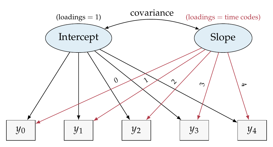
Note. The intercept factor loads on every occasion with a fixed loading of one; the slope factor loads with the time codes (\(0,1,2,3,4\)). The factor means (not shown) carry the average trajectory, the factor variances carry the individual differences, and the factor covariance carries their association. Residuals on each indicator are omitted for clarity. The model is the person-specific line of Chapter 14 written as a factor model.
Seeing the model this way reveals its deepest feature: a growth model is a set of constraints on the moments. The factor structure implies a specific mean vector and covariance matrix for the observed repeated measures, in which the means grow linearly and the variances fan out or in according to the intercept and slope variances and their covariance. Fitting the model tests whether the observed means and covariances match that implied structure, and Figure 19.2 shows the match on the running data: the model-implied means grow linearly through the observed means, and the implied variances track the observed fanning. This implied-moment view is what powers the global fit testing that distinguishes the structural equation approach, because a discrepancy between the observed and implied moments is exactly what the fit indices quantify. In lavaan the model is written either through the convenience function growth, which sets the intercept and slope loadings and the factor means automatically, or by hand, and this chapter teaches the manual specification first so that the convenience is understood rather than trusted.
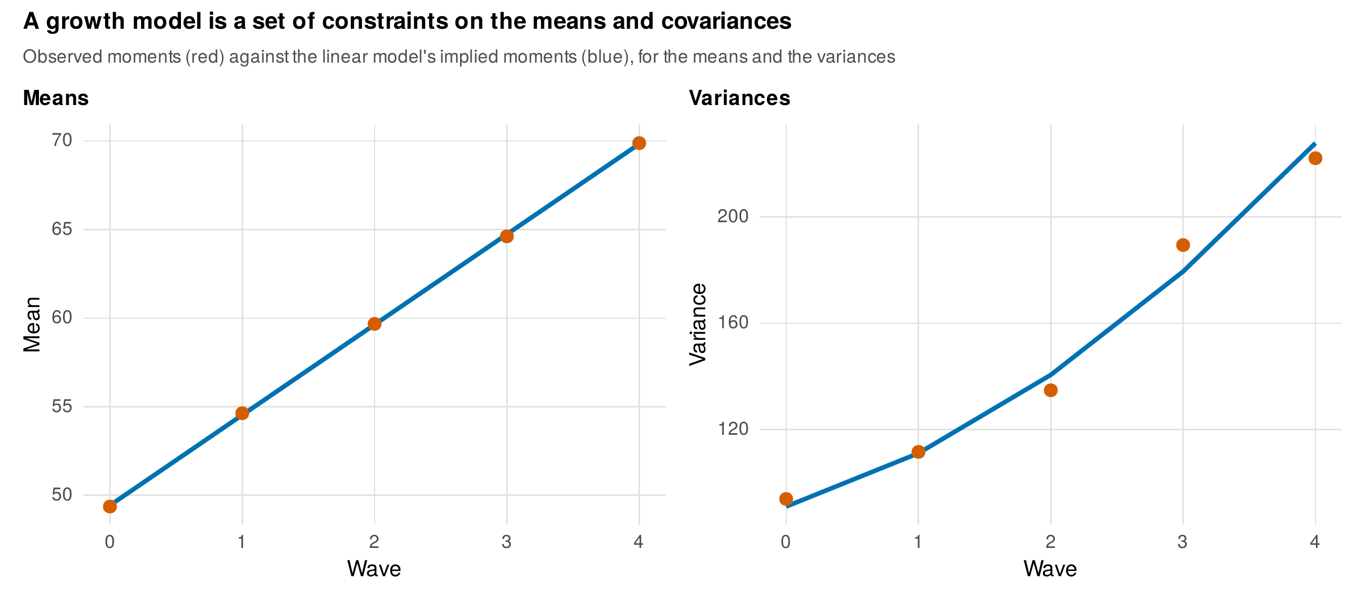
Note. Observed moments (red points) against the implied moments (blue lines) of the linear latent curve model. The model reproduces both the linearly growing means and the fanning variances. A growth model constrains the mean vector and the covariance matrix jointly, and the fit indices quantify the discrepancy between observed and implied.
19.2 Identification and Data Demands
Because a growth model is a set of constraints on the moments, its identification is a matter of counting knowns against unknowns. The knowns are the observed moments: with \(T\) waves there are \(T\) means and \(T(T+1)/2\) variances and covariances. The unknowns are the model parameters: the two factor means, the two factor variances, their covariance, and the residual variances. Table 19.1 works the arithmetic. A linear model with a mean structure is identified with three waves, but only just, leaving no degrees of freedom to test the growth form, so three waves can fit a line but cannot adjudicate whether the line is right. Four waves are the honest minimum for form adjudication, and more are better for nonlinear shapes. A distinct problem is empirical underidentification: when the slope variance is genuinely near zero, the data carry little information about it, and estimation can produce a negative variance estimate, a Heywood case. This is the boundary problem of Chapter 13 in structural-equation clothing, and the response is the same, to diagnose whether the negative estimate reflects a true near-zero variance, sampling noise, or misspecification, and to respond by constraining, simplifying, or, as Chapter 17 showed, moving to Bayesian estimation that keeps the variance in bounds, rather than by panicking or by blindly fixing the estimate to zero.
Table 19.1. Identification arithmetic by waves and growth form.
| Waves | Known moments | Linear parameters | Consequence |
|---|---|---|---|
| Three | \(3 + 6 = 9\) | \(6\) | Just identified for a line; no test of form |
| Four | \(4 + 10 = 14\) | \(6\) | Degrees of freedom to test the form |
| Five or more | Grows quickly | \(6\) (linear) | Room for quadratic, latent basis, and residual freedom |
Note. The known moments are the \(T\) means plus the \(T(T+1)/2\) variances and covariances; the linear model has two factor means, two variances, a covariance, and residual variances. Three waves identify a line but leave nothing to test its shape; four or more are needed to adjudicate the growth form.
19.3 The Equivalence Set Piece
The claim that the multilevel and latent-curve frameworks fit the same model is best demonstrated, not asserted. Fitting the unconditional linear growth model of Chapter 14 to the same data both ways, as a mixed model in lme4 and as a latent curve model in lavaan, returns identical estimates, and Figure 19.3 plots them against each other: every parameter, the intercept and slope means, their variances and covariance, and the residual variance, lies exactly on the line of equality, matching to three decimal places. Table 19.2 is the bilingual dictionary that translates each parameter’s name between the frameworks. The equivalence holds under specific conditions, which are worth stating because their violation is where the frameworks diverge: the time codes must be the same for every person, and the residual structure must match, typically a single residual variance across waves. When those conditions hold the two are the same model estimated by the same likelihood, and the choice between them is one of convenience.
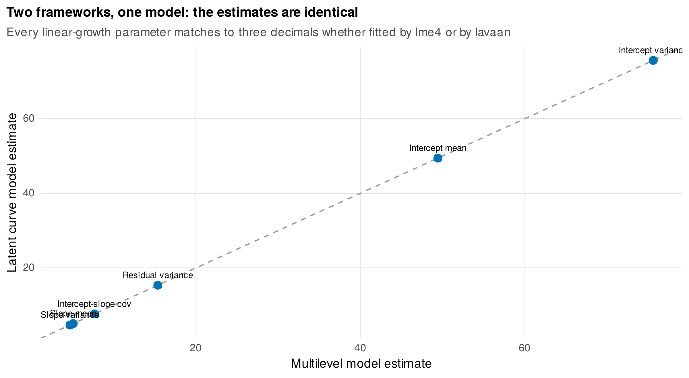
Note. Each parameter of the unconditional linear growth model, estimated as a mixed model (horizontal axis) and as a latent curve model (vertical axis), plotted against the line of equality. Every parameter matches to three decimal places. The two frameworks are dialects of one model when the time codes and residual structure are matched.
Table 19.2. A crosswalk between the multilevel and latent-curve vocabularies.
| Multilevel model | Latent curve model |
|---|---|
| Fixed intercept | Mean of the intercept factor |
| Fixed slope | Mean of the slope factor |
| Random-intercept variance | Variance of the intercept factor |
| Random-slope variance | Variance of the slope factor |
| Intercept-slope covariance | Covariance of the intercept and slope factors |
| Residual variance | Indicator residual variance |
Note. The same six quantities carry different names in the two frameworks. Reading fluently in both is the practical skill this chapter builds; the numbers are identical when the models are matched.
The equivalence has boundaries, and touring them shows what each framework offers. The multilevel framework handles individually varying measurement times natively, because time enters as a numeric predictor that can differ across persons, whereas the standard latent-curve model fixes the time codes in the loadings and so assumes a common schedule; accommodating varying times in the structural equation framework requires definition variables that let each person’s loadings equal their own measurement times, available in some programs and a genuine limitation of others (Mehta & Neale, 2005; Mehta & West, 2000). The structural equation framework, in turn, supplies global fit machinery that the multilevel framework lacks, and this is not idle, because it detects misspecification of the growth form that a multilevel model, which does not test the implied covariance structure against the observed, can miss. The structural equation framework also embeds the growth factors in larger structural systems, letting a slope factor predict a distal outcome or mediate an effect, which the multilevel framework cannot do directly. Both handle structured residuals, with different ergonomics, and both default to full-information maximum likelihood under missingness. Table 19.3 is the decision guide, and the book’s position is bilingualism: the frameworks are dialects, not denominations (Curran, 2003; Bauer, 2003; McNeish & Matta, 2018).
Foundations Box • The implied moments and the equivalence
For a linear model with time codes \(a_t\), the implied mean at wave \(t\) is \(\mu_t = \gamma_I + \gamma_S a_t\), where \(\gamma_I\) and \(\gamma_S\) are the intercept and slope factor means, so the implied means are a straight line in the time codes. The implied covariance between waves \(s\) and \(t\) is \(\tau_{II} + (a_s + a_t)\tau_{IS} + a_s a_t\,\tau_{SS} + \sigma^2\mathbb{1}(s=t)\), where \(\tau_{II}\), \(\tau_{SS}\), and \(\tau_{IS}\) are the factor variances and covariance and \(\sigma^2\) is the residual variance. This is exactly the marginal covariance \(\mathbf{Z}\mathbf{T}\mathbf{Z}' + \sigma^2\mathbf{I}\) that Chapter 13 derived for the random-slope mixed model, with \(\mathbf{Z}\) the matrix of time codes and \(\mathbf{T}\) the factor covariance matrix. The two frameworks therefore impose the identical mean vector and covariance matrix on the data and, fitting by the same maximum-likelihood criterion, return the identical estimates. The equivalence breaks exactly when the two implied structures differ: when the time codes vary across persons, so \(\mathbf{Z}\) is not common, or when the residual structure differs from \(\sigma^2\mathbf{I}\) in a way one framework parameterizes and the other does not.
Table 19.3. Choosing the multilevel or the structural-equation framework.
| Favor the multilevel framework when | Favor the structural-equation framework when |
|---|---|
| Measurement times vary across persons | The growth form must be tested against global fit |
| Occasions are many and unbalanced | Growth factors predict or mediate other variables |
| Three or more levels of nesting | Multiple groups or parallel processes are compared |
| The question is about fixed and random effects | The shape of change is to be estimated (latent basis) |
Note. The frameworks are equivalent for the common case and diverge at the edges. The multilevel framework excels at unbalanced designs and varying times; the structural-equation framework at global fit, structural embedding, and multiple-group and parallel-process extensions. The fluent researcher uses both.
19.4 Fit Evaluation for Growth Models
Because a growth model constrains the means and the covariances jointly, its fit indices carry information the multilevel framework does not surface, but they must be read with care. A poor comparative fit index or a large root mean square error of approximation signals that the implied moments do not match the observed, and the first diagnostic question is where: misfit in a growth model is often in the mean structure, an average trajectory of the wrong shape, rather than in the covariances. The forensic tool is to inspect the residual moments, the differences between observed and implied means and covariances, to localize the discrepancy. Figure 19.4 shows the diagnosis on a decelerating outcome fitted with a linear model: the linear model’s implied means bow systematically away from the observed means, over-predicting in the middle and under-predicting at the ends, the fingerprint of a wrong growth form, while a model that estimates the shape reproduces the means. The benchmarks for the fit indices carry the same cautions rehearsed in Chapter 18, that they are rules of thumb from particular conditions, and they are sensitive here to the sample size and to the magnitude of the slope variance. Nested models for the growth form, linear against a freed-loading shape against a quadratic, are compared by the chi-square difference and the information criteria. Table 19.4 is the protocol, and a recurring lesson is that good global fit does not certify the correct growth form, only that the chosen form is not grossly contradicted (Wu et al., 2009).
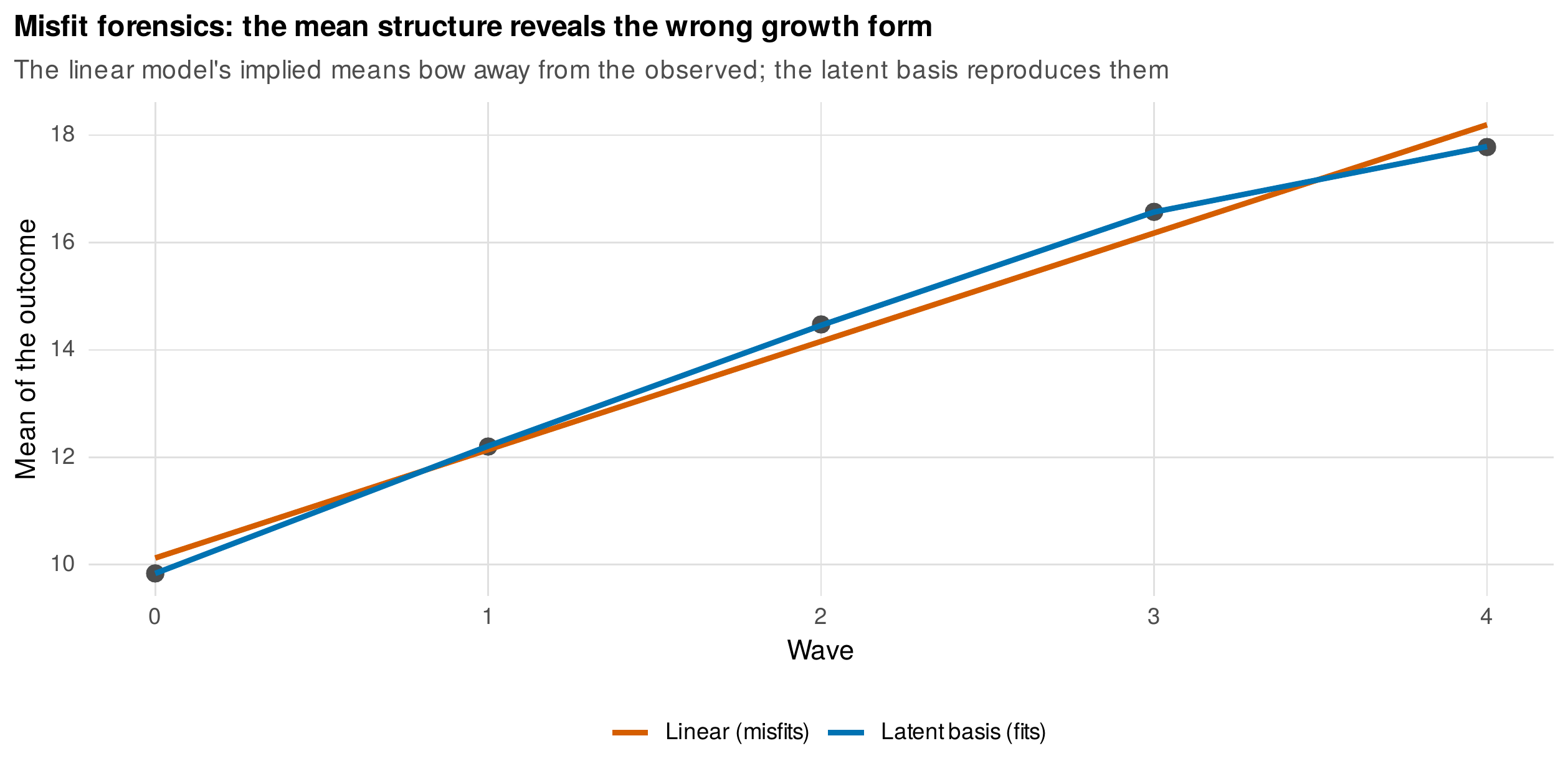
Note. Observed means (grey points) of a decelerating outcome against the implied means of a linear model (red) and a freed-loading model (blue). The linear model’s implied means bow away from the observed, the signature of a misspecified growth form, which resides in the mean structure; the freed-loading model reproduces the means. Locate growth-model misfit by inspecting the residual moments.
Table 19.4. A fit-evaluation protocol for growth models.
| Step | What to do |
|---|---|
| Global indices | Read the chi-square, CFI, RMSEA, and SRMR against benchmarks, as diagnostics |
| Locate misfit | Inspect the residual means and covariances to find where the model departs |
| Mean versus covariance | Decide whether misfit is in the trajectory shape or the individual differences |
| Compare forms | Test linear against latent-basis against quadratic by chi-square difference and information criteria |
| Guard the conclusion | Remember that good fit does not certify the growth form |
Note. Growth-model misfit is frequently in the mean structure, so the residual-moment inspection is essential. The fit indices are sensitive to sample size and to the slope-variance magnitude, and good fit is necessary but not sufficient for the correct growth form.
19.5 Conditional Models and Consequences of Growth
A conditional growth model adds covariates that predict the growth factors, and it is the structural-equation counterpart of the cross-level interactions of Chapter 14, the same estimand in different clothing. A time-invariant covariate regressed on the intercept and slope factors gives its effect on the starting level and on the rate of change, and Figure 19.5 shows the predicted trajectories at several covariate values, diverging because the covariate raises the slope. On the running data the covariate’s effect on the slope factor recovers its true value. Time-varying covariates enter as occasion-specific predictors of the repeated measures, carrying the same warnings rehearsed in Chapter 14, that a covariate trending with time can absorb the growth it should sit alongside. The distinctive structural-equation extension is to place the growth factors as predictors of a distal outcome, the slope-as-predictor model in which the rate of change forecasts a later result. This is powerful and hazardous: the slope factor is estimated with error, so its reliability bounds what it can predict, and the time window matters, because predicting an outcome from change measured over an interval that overlaps the outcome courts circularity. These cautions are the price of the structural-equation framework’s reach.
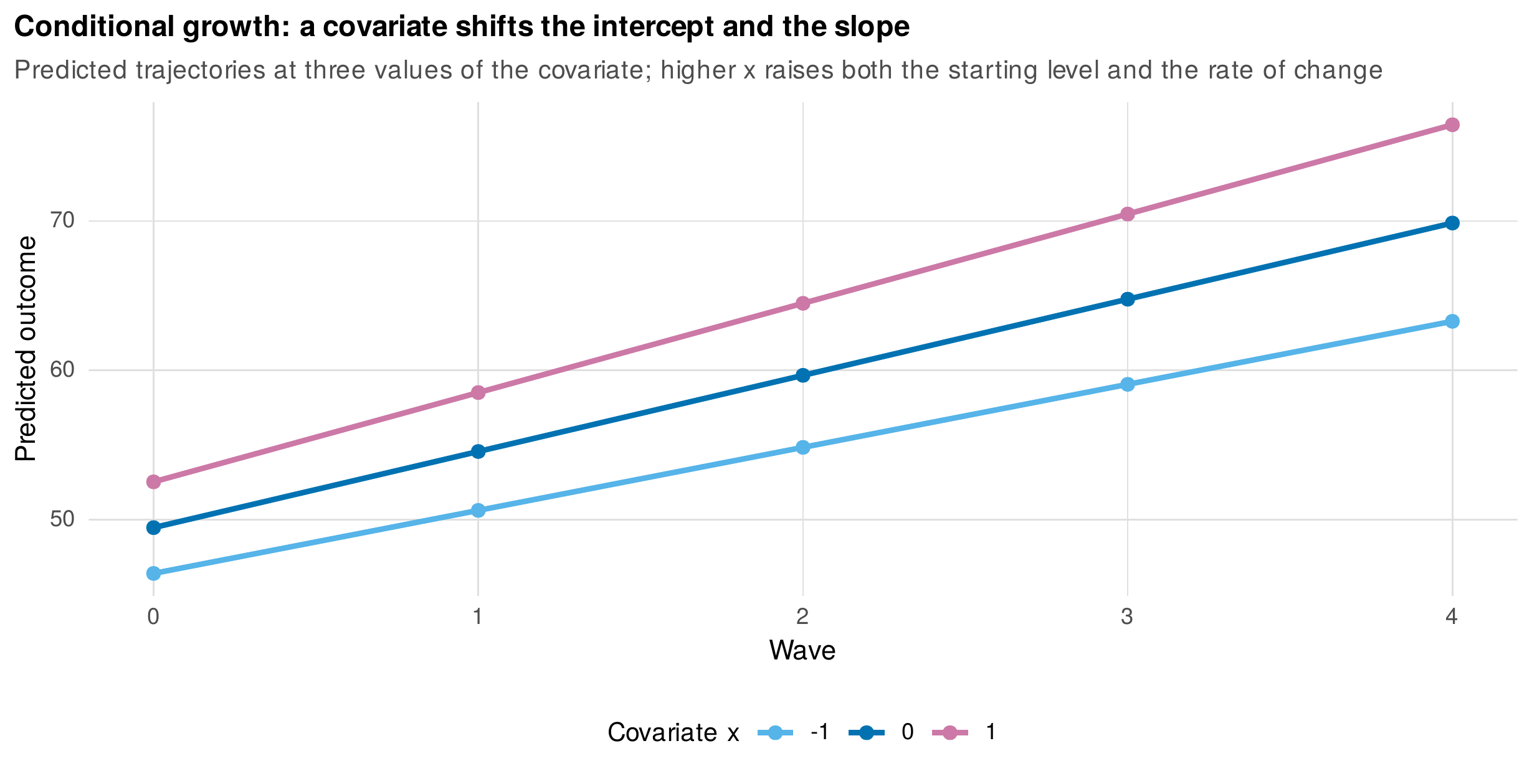
Note. Predicted trajectories at three values of a time-invariant covariate that is regressed on the intercept and slope factors. A higher covariate value raises both the starting level and the rate of change, so the trajectories diverge. This is the latent-curve counterpart of the cross-level interaction of Chapter 14.
19.6 Multiple-Group Growth
Fitting a growth model in multiple groups compares trajectories across, for instance, the arms of a trial, and it makes the treatment effect a difference in the slope-factor mean. Figure 19.6 shows the arm-specific fitted trajectories on the therapy trial of Chapter 14, now analyzed as a multiple-group latent curve model with full-information maximum likelihood for the dropout, and the treatment arm’s steeper decline, a slope of about one point per week faster than the control arm, is the treatment effect. The analysis proceeds by a constraint-testing sequence, from a configural model with the growth form free in each group, to a model constraining the growth-factor means equal, and the test of that constraint is the test of the treatment effect, which here rejects equality decisively. Table 19.5 lays out the sequence. This multiple-group parameterization is exactly equivalent to the arm-by-time interaction of the Chapter 14 conditional model, the treatment effect appearing as an interaction in one framework and as a group difference in slope means in the other, and demonstrating that equivalence again is part of the bilingual discipline. When the construct is measured by multiple items, the comparison rests on the measurement invariance of Chapter 18, and the full chain, invariant measurement supporting comparable growth factors, is the second-order growth model developed in Chapter 20.
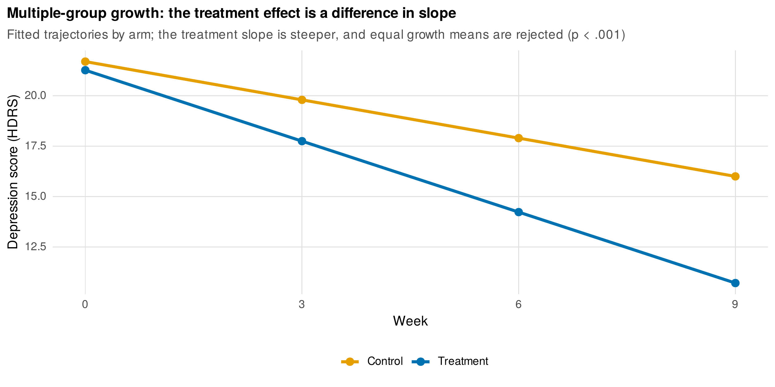
Note. Fitted trajectories for the two arms of the therapy trial, from a multiple-group latent curve model with full-information maximum likelihood. The treatment arm declines faster, and the test constraining the growth-factor means equal across arms rejects, establishing the treatment effect. This parameterization is equivalent to the arm-by-time interaction of Chapter 14.
Table 19.5. A constraint sequence for multiple-group growth.
| Model | Constrains across groups | Tests |
|---|---|---|
| Configural | Nothing (same form) | Whether the form holds in each group |
| Equal variances | Factor variances | Equal individual differences in growth |
| Equal means | Factor means | Equal average trajectories (the group effect) |
Note. The treatment or group effect is the test of equal growth-factor means. When the outcome is multi-item, measurement invariance (Chapter 18) must hold first, and the full chain is the second-order growth model of Chapter 20.
19.7 Parallel-Process Growth
A parallel-process model fits growth in two domains at once and estimates the associations among their growth factors, including the slope-slope covariance that asks whether change in one domain accompanies change in the other. Figure 19.7 shows the estimated growth slopes of two outcomes plotted against each other, with a positive association: people whose first outcome grows faster tend to have a faster-growing second outcome. The interpretive caution is essential and easily forgotten. A slope-slope correlation is a statement of correlated change, that two processes move together across people, and it is not evidence that one process drives the other. Establishing which process leads requires a model of the temporal dynamics, the lead-lag structure that a static association cannot reveal, and that is precisely what the latent change score and cross-lagged panel models of Chapters 20 and 21, and the dynamic models of the intensive-longitudinal part, are built to provide. The parallel-process model describes the coupling; it does not explain it, and reporting it as though it did is a common overreach.
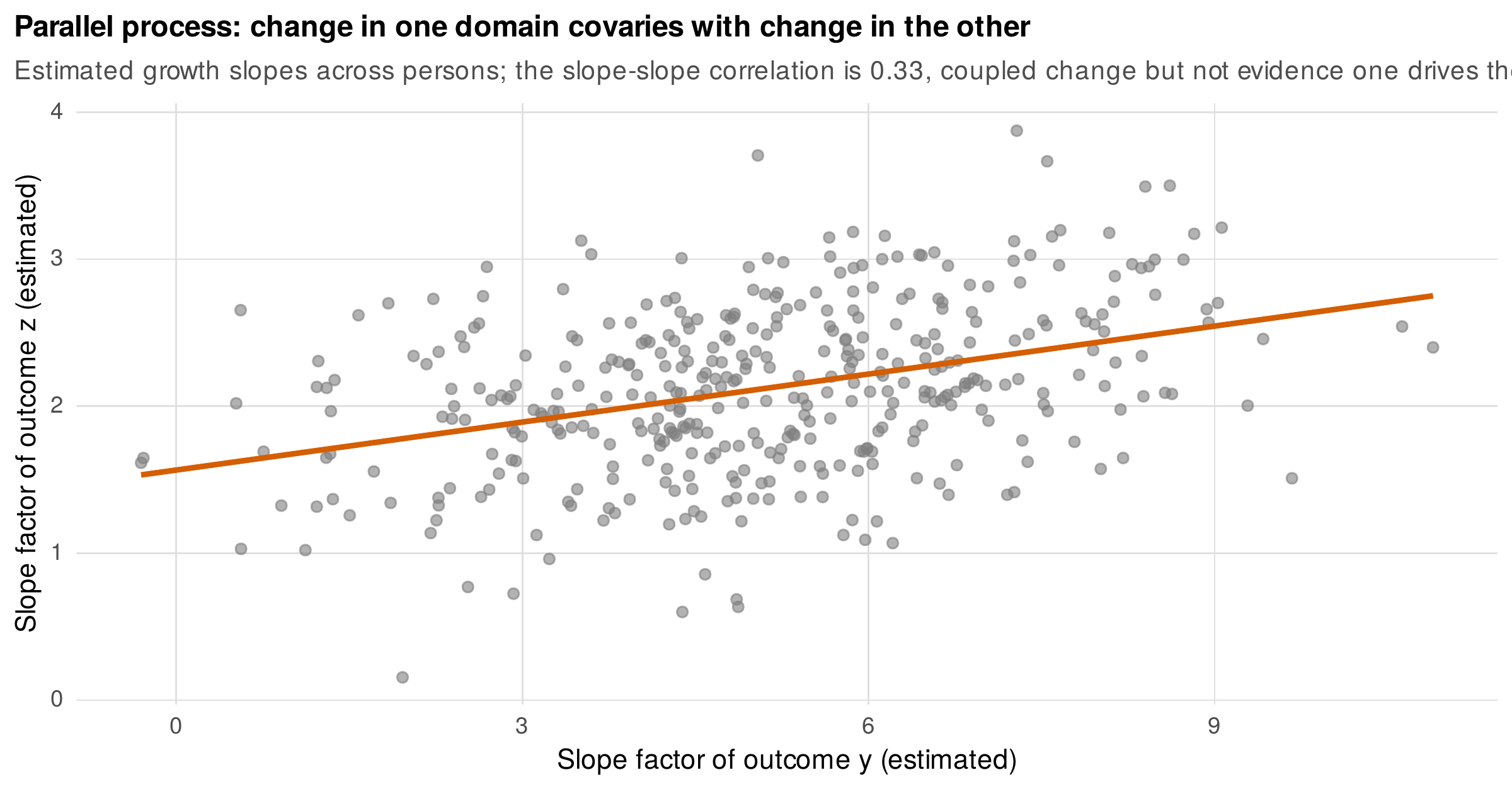
Note. Estimated growth slopes of two outcomes across persons, with their positive association. The slope-slope correlation describes correlated change, that the two processes move together, and is not evidence that one drives the other. Establishing direction requires the dynamic models of the chapters to come.
19.8 Latent-Basis Growth
When the shape of change is unknown, the structural equation framework can estimate it rather than impose it, through a latent-basis or freed-loading model. The first and last slope loadings are fixed, to zero and one, so that the slope factor represents the total change from the first occasion to the last, and the interior loadings are freed and estimated, so that each interior loading is the proportion of the total change that has occurred by that wave. Figure 19.8 shows the result on a decelerating outcome: the freed loadings recover the true nonlinear shape, and they differ visibly from the equal spacing a linear model would impose. On the running data the latent-basis model fits better than the linear model and comparably to a quadratic, at fewer parameters. The freed-loading approach has real power, giving an interpretable proportion-of-change reading and adapting to any monotone shape, but it carries traps. It capitalizes on chance, fitting the sample’s particular shape, so the estimated basis should be cross-validated or theoretically motivated; and comparing a latent basis across groups requires constraining the loadings, because an unconstrained basis that differs across groups conflates a difference in shape with a difference in the measurement of change. Used with these cautions, the latent basis is often preferable to a polynomial, which imposes a rigid functional form and extrapolates poorly.
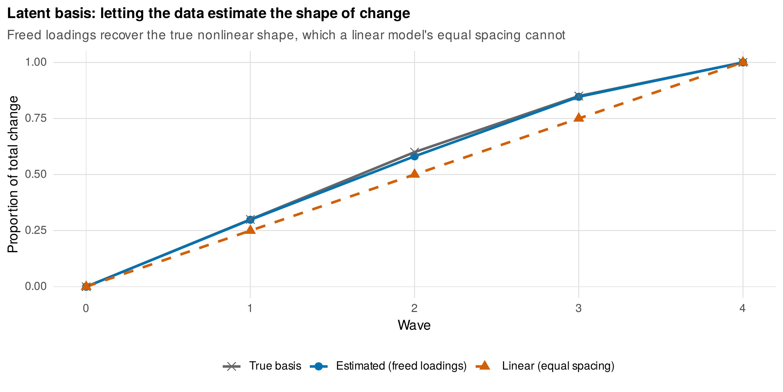
Note. The estimated freed loadings (blue), the true shape (grey), and the equal spacing a linear model imposes (red), as proportions of the total change by wave. The freed loadings recover the true nonlinear shape, which the linear model cannot. Each interior loading reads as the proportion of total change achieved by that wave.
19.9 Reporting a Latent Growth Analysis
A latent growth analysis is reported so that its constraints and choices are legible, and Table 19.6 is the checklist. The report states the time coding and its origin, because every intercept-related quantity depends on it exactly as in Chapter 14; names the growth form and the basis for choosing it; gives the factor means, variances, and covariance with the average trajectory and the individual differences interpreted; reports the global fit with the residual-moment diagnosis where fit is imperfect; describes the missing-data handling; and, for conditional, multiple-group, or parallel-process extensions, reports the relevant coefficients, constraint tests, or factor associations with their cautions. Where the frameworks are equivalent, noting the correspondence with the multilevel parameterization aids a bilingual readership.
Table 19.6. A reporting checklist for a latent growth analysis.
| Element | What to report |
|---|---|
| Time coding and origin | The metric, its units, and where time is zero |
| Growth form | The shape and the basis for selecting it |
| Factor means | The average intercept and slope, the average trajectory |
| Factor variances and covariance | The individual differences and their association, at the stated origin |
| Fit and misfit | The global indices and the residual-moment diagnosis |
| Missing data | The estimator, typically full-information maximum likelihood |
| Extensions | Conditional coefficients, constraint tests, or factor associations, with cautions |
Note. The checklist extends the growth-model reporting of Chapter 14 to the structural-equation quantities: global fit and its localization, and the factor parameterization. Noting the multilevel correspondence serves a bilingual readership.
19.10 Running Latent Growth Models in R
The lavaan package fits the model through the convenience function growth, which sets the intercept and slope loadings and estimates the factor means, or through manual syntax that makes every constraint explicit.
library(lavaan)
lgm <- '
  I =~ 1*y0 + 1*y1 + 1*y2 + 1*y3 + 1*y4          # intercept: loadings all 1
  S =~ 0*y0 + 1*y1 + 2*y2 + 3*y3 + 4*y4          # slope: loadings = time codes
  y0 ~~ r*y0; y1 ~~ r*y1; y2 ~~ r*y2             # equal residuals (to match the mixed model)
  y3 ~~ r*y3; y4 ~~ r*y4
  I ~ 1; S ~ 1                                    # the mean structure: factor means '
fit <- growth(lgm, data = wide)                   # or sem(lgm, ..., meanstructure = TRUE)
summary(fit, fit.measures = TRUE, standardized = TRUE)
Conditional, multiple-group, parallel-process, and latent-basis models are small extensions of this syntax: a covariate is regressed on the factors (I x; S x); groups are compared with the group and group.equal arguments; a parallel process adds a second pair of factors; and a latent basis frees the interior loadings (S = 0*y0 + NA*y1 + NA*y2 + NA*y3 + 1*y4).
growth(lgm, data = wide, group = "arm", missing = "fiml")   # multiple-group, FIML
anova(fit_configural, fit_equalmeans)                        # test the group effect
# equivalence check: the same model as a mixed model
library(lme4); lmer(y ~ wave + (wave | id), data = long)
The complete analysis, including the parameter-by-parameter equivalence with lme4, the moment inspection, the conditional and multiple-group and parallel-process models, and the latent-basis shape recovery, is the shipped script ch19_analysis_V01.R, with figures drawn by ch19_figures_V01.R and the dataset generated by gen_growth_wide_V01.R.
Software Note • latent growth across programs
The model is fitted by growth or sem in lavaan, by PROC CALIS in SAS, and by the MODEL command in Mplus, whose i s | y0@0 y1@1 ... syntax names the intercept and slope factors compactly and whose TSCORES option supplies individually varying times through definition variables, the feature the standard lavaan model lacks. The OpenMx package implements definition variables directly and so fits growth with person-specific measurement times, the structural-equation route to the individually varying occasions that the multilevel framework handles natively. For the routine linear and polynomial models, lavaan and the multilevel packages are interchangeable, and the choice follows the ergonomics of the surrounding analysis; the MplusAutomation package supports a round-trip workflow for laboratories standardized on Mplus.
19.11 Common Misconceptions
Several beliefs about latent growth models mislead. The first is that structural-equation growth modeling is more advanced or more correct than multilevel growth modeling; the two are the same model under matched assumptions, and they differ only in ergonomics (Figure 19.3). The second is that a poor comparative fit index kills the growth model; misfit should first be localized, because it often lies in the mean structure and signals the wrong growth form rather than a fatal flaw. The third is that a nonzero slope variance proves individual differences in change exist; the variance is estimated with error and can hit a boundary, so its precision, and the power to detect it, must be weighed. The fourth is that a parallel-process slope correlation shows one domain drives the other; it shows correlated change, and direction requires a dynamic model. The fifth is that good fit certifies the growth form; good fit is necessary but not sufficient, and a well-fitting linear model can still be the wrong shape at unobserved times.
Common Pitfall • four errors in latent growth practice
First, interpreting the intercept-slope correlation without stating the time origin: as in Chapter 14, the correlation depends on where time is coded zero, so the origin must be named. Second, panicking at a Heywood case: a negative variance estimate calls for diagnosis, whether it reflects a true near-zero variance, sampling noise, or misspecification, not a reflexive fix. Third, comparing latent-basis loadings across groups without constraining them: an unconstrained basis conflates a difference in shape with a difference in the measurement of change. Fourth, treating a parallel-process correlation as a causal coupling: correlated change is not a lead-lag relationship.
Chapter Summary
The latent growth curve model represents change through an intercept factor with unit loadings and a slope factor with loadings fixed to the time codes, and its distinctive requirement is the mean structure, because the average trajectory is carried by the factor means (Figure 19.1). The model constrains the observed means and covariances jointly, which is what powers its global fit testing (Figure 19.2), and it is identified with three waves for a line but needs four or more to test the form (Table 19.1). It is the same model as the multilevel growth model of Chapter 14 under matched time codes and residual structure, returning identical estimates (Figure 19.3, Table 19.2), and it diverges where the multilevel framework’s varying times or the structural-equation framework’s global fit, structural embedding, and multiple-group and parallel-process extensions come into play (Table 19.3). Its fit is evaluated by localizing misfit in the mean structure (Figure 19.4, Table 19.4). Covariates predict the growth factors in a conditional model, the counterpart of the cross-level interaction (Figure 19.5); groups are compared with a constraint sequence that makes a treatment effect a slope-mean difference (Figure 19.6, Table 19.5); parallel processes reveal correlated but not causally coupled change (Figure 19.7); and freed loadings estimate a nonlinear shape as proportions of total change (Figure 19.8). The frameworks are dialects of one language, and fluency in both is the chapter’s aim.
Where to Go Next
This chapter and Chapter 14 together complete the growth-modeling core in both dialects. Chapter 20 extends the latent-curve framework in two directions: the second-order growth model that fits the trajectory to the invariant latent factors of Chapter 18, cashing the measurement check that a composite score silently assumes, and the latent change score model that reparameterizes growth as a sequence of change scores and so begins to model the dynamics of change rather than only its shape. Chapter 21 places growth factors inside the cross-lagged panel systems that ask which process leads, resolving the directional question the parallel-process model can only raise. Chapter 22 asks whether a single growth model conceals a mixture of distinct trajectory classes. Throughout, the bilingual habit this chapter builds, seeing every growth model as both a mixed model and a set of constraints on the moments, is the working competence of longitudinal structural equation modeling.
Exercises
- 19.1 Implied moments by hand. For a four-wave linear model with given factor means, variances, covariance, and residual variance, compute the implied mean vector and covariance matrix, and verify them against a
lavaanfit. - 19.2 Reproduce and break the equivalence. Fit the unconditional linear model as a mixed model and a latent curve model and confirm the estimates match; then add an autoregressive residual structure and explain why the equivalence no longer holds.
- 19.3 Misfit forensics. Fit a linear model to a dataset with a planted quadratic shape, and use the residual moments to locate and diagnose the misfit.
- 19.4 Multiple-group analysis. Fit a multiple-group growth model with the constraint sequence, test the group effect, and write the results, noting the equivalence with the interaction parameterization.
- 19.5 Latent basis. Fit a freed-loading model, interpret the loadings as proportions of total change, and compare it to a quadratic by fit and parsimony.
- 19.6 Bilingual translation. Translate a published multilevel growth table into latent-curve syntax and confirm the two produce the same estimates.
References
Bauer, D. J. (2003). Estimating multilevel linear models as structural equation models. Journal of Educational and Behavioral Statistics, 28(2), 135–167. https://doi.org/10.3102/10769986028002135
Bollen, K. A., & Curran, P. J. (2006). Latent curve models: A structural equation perspective. Wiley. https://doi.org/10.1002/0471746096
Chou, C.-P., Bentler, P. M., & Pentz, M. A. (1998). Comparisons of two statistical approaches to study growth curves: The multilevel model and the latent curve analysis. Structural Equation Modeling, 5(3), 247–266. https://doi.org/10.1080/10705519809540104
Curran, P. J. (2003). Have multilevel models been structural equation models all along? Multivariate Behavioral Research, 38(4), 529–569. https://doi.org/10.1207/s15327906mbr3804_5
Duncan, T. E., Duncan, S. C., & Strycker, L. A. (2006). An introduction to latent variable growth curve modeling: Concepts, issues, and applications (2nd ed.). Erlbaum. https://doi.org/10.4324/9780203879962
Grimm, K. J., Ram, N., & Estabrook, R. (2017). Growth modeling: Structural equation and multilevel modeling approaches. Guilford Press.
McArdle, J. J. (2009). Latent variable modeling of differences and changes with longitudinal data. Annual Review of Psychology, 60(1), 577–605. https://doi.org/10.1146/annurev.psych.60.110707.163612
McArdle, J. J., & Epstein, D. (1987). Latent growth curves within developmental structural equation models. Child Development, 58(1), 110–133. https://doi.org/10.2307/1130295
McNeish, D., & Matta, T. (2018). Differentiating between mixed-effects and latent-curve approaches to growth modeling. Behavior Research Methods, 50(4), 1398–1414. https://doi.org/10.3758/s13428-017-0976-5
Mehta, P. D., & Neale, M. C. (2005). People are variables too: Multilevel structural equations modeling. Psychological Methods, 10(3), 259–284. https://doi.org/10.1037/1082-989X.10.3.259
Mehta, P. D., & West, S. G. (2000). Putting the individual back into individual growth curves. Psychological Methods, 5(1), 23–43. https://doi.org/10.1037/1082-989X.5.1.23
Meredith, W., & Tisak, J. (1990). Latent curve analysis. Psychometrika, 55(1), 107–122. https://doi.org/10.1007/BF02294746
Preacher, K. J., Wichman, A. L., MacCallum, R. C., & Briggs, N. E. (2008). Latent growth curve modeling. Sage. https://doi.org/10.4135/9781412984737
Rosseel, Y. (2012). lavaan: An R package for structural equation modeling. Journal of Statistical Software, 48(2), 1–36. https://doi.org/10.18637/jss.v048.i02
Willett, J. B., & Sayer, A. G. (1994). Using covariance structure analysis to detect correlates and predictors of individual change over time. Psychological Bulletin, 116(2), 363–381. https://doi.org/10.1037/0033-2909.116.2.363
Wu, W., West, S. G., & Taylor, A. B. (2009). Evaluating model fit for growth curve models: Integration of fit indices from SEM and MLM frameworks. Psychological Methods, 14(3), 183–201. https://doi.org/10.1037/a0015858