Chapter 20
Latent Change Score and Advanced Growth Models
The growth models of the previous chapters describe trajectories: they say what the average path looks like and how people vary around it. This chapter models something different, the rule that generates change from one occasion to the next. A latent change score model treats the change between adjacent true scores as a variable in its own right and writes an equation for it, most often that the change is part a constant increment and part a proportion of the current level. That single move, from describing the trajectory to specifying the rule that produces it, is a shift from a kinematic to a dynamic way of thinking, and it is the conceptual hinge between the trajectory models of Part V and the dynamic models of Part VI. Change as a function of the current state is a difference equation, the discrete-time cousin of the differential equations that the continuous-time models of Chapter 27 will write, and saying so out loud reframes growth modeling as the study of a system’s dynamics. The chapter develops the univariate change score model and its trajectory taxonomy, extends it to two coupled processes where the celebrated and much-abused question of which process leads the other arises, insists on a sensitivity discipline that the coupling literature has too often skipped, and then cashes the measurement check of Chapter 18 in the second-order growth model that fits change to an invariant latent construct rather than to a fallible composite.
Learning Objectives
After working through this chapter, you should be able to: (1) specify a univariate latent change score model with its true-score layer, fixed unit paths, and latent difference variables, and derive how constant and proportional change generate a family of trajectory shapes; (2) interpret the additive and proportional change parameters and their dependence on the observation interval; (3) fit a bivariate change score model with coupling parameters and interpret a lead-lag claim with the required cautions; (4) run a coupling-sensitivity battery; (5) construct a second-order growth model on invariant measurement and state its advantages; and (6) fit these models in R using a reusable syntax generator.
20.1 Change as a Latent Variable
The latent change score model, developed in a long program by McArdle and colleagues (McArdle, 2009; McArdle & Hamagami, 2001), is built from a scaffolding that novices find alien because nearly every path in it is fixed to one. Figure 20.1 draws it. Behind each observed score sits a latent true score, freed of measurement error, and the true scores are connected across time by autoregressions whose coefficient is fixed to exactly one, so that each true score carries forward the entire previous true score unchanged. Into each true score flows a latent change score, again with a path fixed to one, so that the true score at each occasion is literally the previous true score plus the change, an accounting identity rather than a regression. The modeling happens on the change scores. A constant change factor loads on every change score with a fixed loading of one, contributing the same increment at each step, and its mean is the additive change parameter. A proportional change path runs from each true score to the next change score with a coefficient, the same at every interval, that makes part of each change a proportion of the current level. The fixed ones are not arbitrary: they enforce the identity that change is the difference of adjacent true scores, so that the free parameters, the mean and variance of the constant change and the proportional coefficient, are the actual objects of inference.
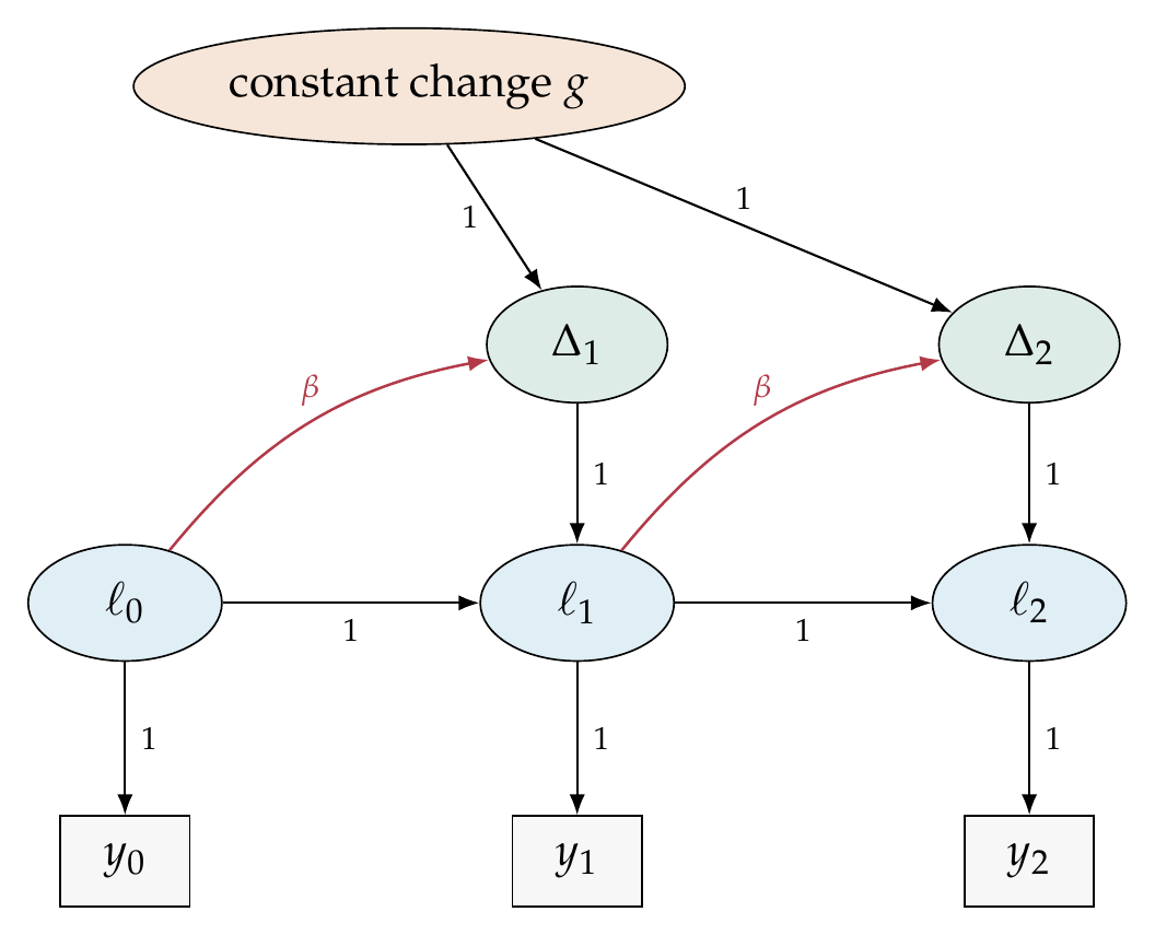
Note. Latent true scores \(\ell_t\) underlie the observed scores \(y_t\) with loadings fixed to one; the autoregressions between true scores are fixed to one; each latent change score \(\Delta_t\) enters its true score with a path fixed to one, enforcing the identity \(\ell_t = \ell_{t-1} + \Delta_t\). The free parameters are on the change: the constant-change factor \(g\) (loadings one, mean the additive change) and the proportional coefficient \(\beta\) (red) from the previous level. The fixed ones are what make change a modeled latent variable.
Writing the change rule as \(\Delta_t = g + \beta\,\ell_{t-1}\) and unrolling it reveals why this apparatus is worth the trouble: a handful of parameters generate a whole family of trajectory shapes. When only the constant change is present, the trajectory is linear, the same increment at every step. When only proportional change is present, the trajectory is a geometric approach, decaying toward zero if the coefficient is negative or exploding if positive. When both are present, the dual change model, the trajectory approaches an asymptote at \(-g/\beta\), rising or falling toward it at a decelerating rate, the negative-exponential shape that Chapter 14 fitted directly as a nonlinear mixed model. Figure 20.2 draws the taxonomy, one equation producing constant, decaying, asymptotic, and accelerating trajectories according to the sign and size of the proportional coefficient, and Table 20.1 maps the change-score parameterization onto the nonlinear-curve parameterization of Chapter 14. The two describe the same curves; the change score model just reaches them through the rule that generates them rather than through the function they trace.
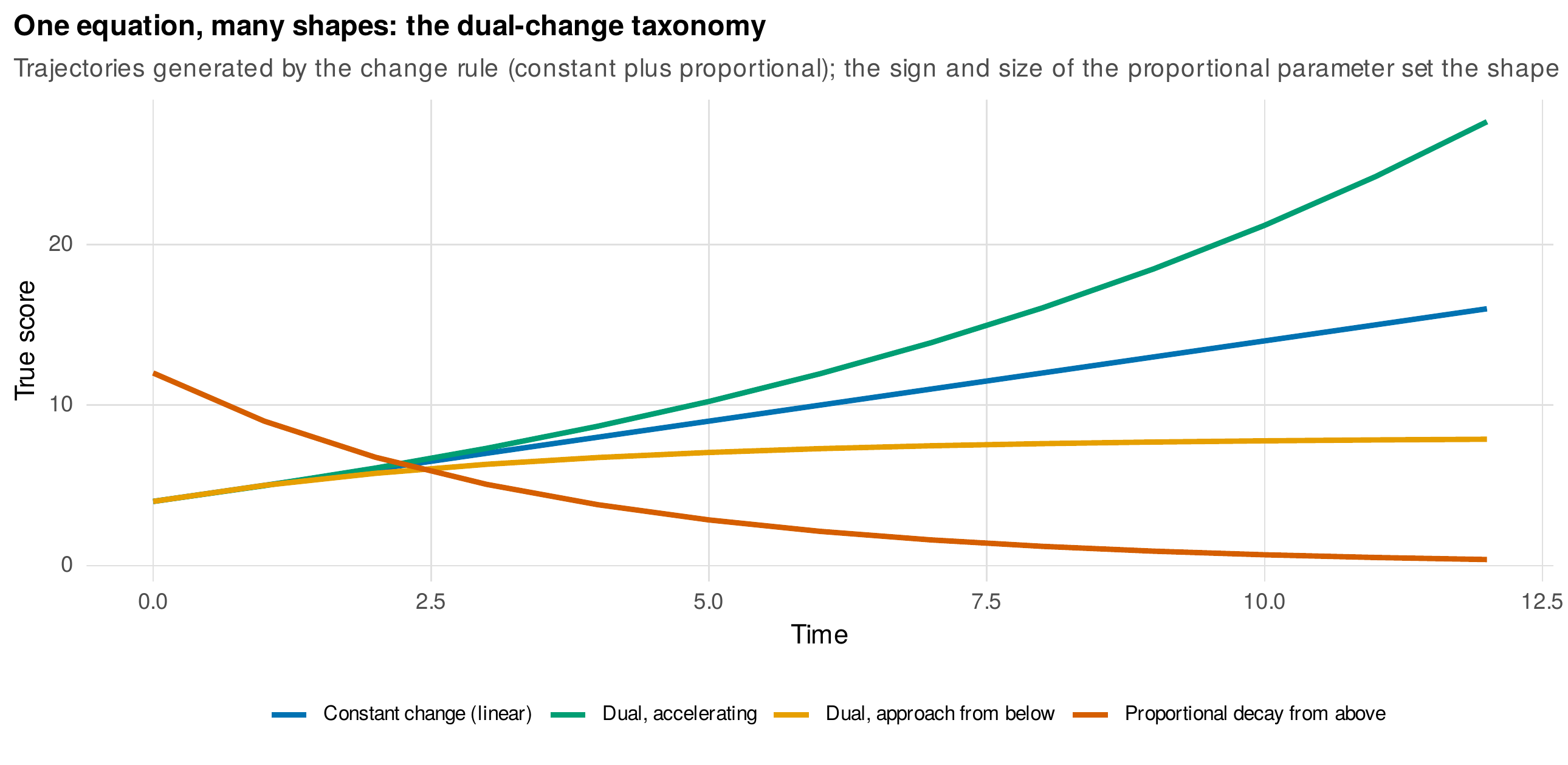
Note. Trajectories generated by the change rule \(\Delta_t = g + \beta\,\ell_{t-1}\). A zero proportional coefficient gives linear change; a negative coefficient with no constant gives decay; a positive constant with a negative coefficient gives an asymptotic approach; a positive coefficient gives acceleration. The generative rule, not a fitted function, produces the family.
Foundations Box • From the difference equation to the trajectory, and to continuous time
The dual-change rule \(\Delta_t = \ell_t - \ell_{t-1} = g + \beta\,\ell_{t-1}\) rearranges to the linear recurrence \(\ell_t = (1+\beta)\,\ell_{t-1} + g\), whose solution is \(\ell_t = (1+\beta)^t\left(\ell_0 + g/\beta\right) - g/\beta\). When \(-2 < \beta < 0\) the factor \((1+\beta)^t\) decays, so \(\ell_t\) approaches the equilibrium \(-g/\beta\) geometrically, the discrete-time image of exponential approach. This is the solved trajectory, the same negative-exponential curve of Chapter 14 with the correspondence of Table 20.1. The discrete recurrence is an approximation to the continuous-time differential equation \(d\ell/dt = a + b\,\ell\), whose solution \(\ell(t) = e^{bt}(\ell_0 + a/b) - a/b\) replaces the discrete \((1+\beta)^t\) with the continuous \(e^{bt}\). The two agree only as the observation interval shrinks, which is exactly why the discrete proportional coefficient depends on the sampling interval while the continuous rate does not, the issue that Chapter 27 resolves.
Table 20.1. Change-score and nonlinear-curve parameterizations of the same trajectories.
| Change rule | Implied trajectory | Chapter 14 counterpart |
|---|---|---|
| Constant only (\(\beta=0\)) | Linear | Linear growth |
| Proportional only | Geometric decay or growth | Exponential from a zero asymptote |
| Dual change (\(g\) and \(\beta\)) | Approach to an asymptote \(-g/\beta\) | Negative-exponential growth |
Note. The latent change score model reaches the same curves as the nonlinear mixed models of Chapter 14 through the rule that generates change rather than through the function it traces. The asymptote of a dual-change process is \(-g/\beta\).
20.2 Univariate Change Score Models in Practice
Fitting the specification ladder to data with a known decelerating rise makes the choice concrete. On the running dataset, a simulated process generated by a dual-change rule, the constant-change model fits poorly because it forces a straight line through a curved trajectory, the proportional-only model fits worse still because without a constant increment it cannot capture the sustained rise, and the dual-change model fits well and recovers the generating parameters, an additive change near its true value and a proportional coefficient near its true negative value. Figure 20.3 shows the three implied trajectories against the observed means: only the dual-change model tracks the deceleration. The comparison is by the information criteria and, where the models are nested, by the chi-square difference, and the dual-change model is preferred by a wide margin. Table 20.2 is the parameter glossary, and Table 20.3 maps parameter configurations to dynamics. Two estimation pathologies recur and deserve calm responses rather than alarm: the proportional coefficient can drift to a boundary when the data are nearly linear, and a change-score variance can go slightly negative, the boundary problem of Chapter 13 again, to be met by simplifying the model or, as Chapter 17 showed, by Bayesian estimation.
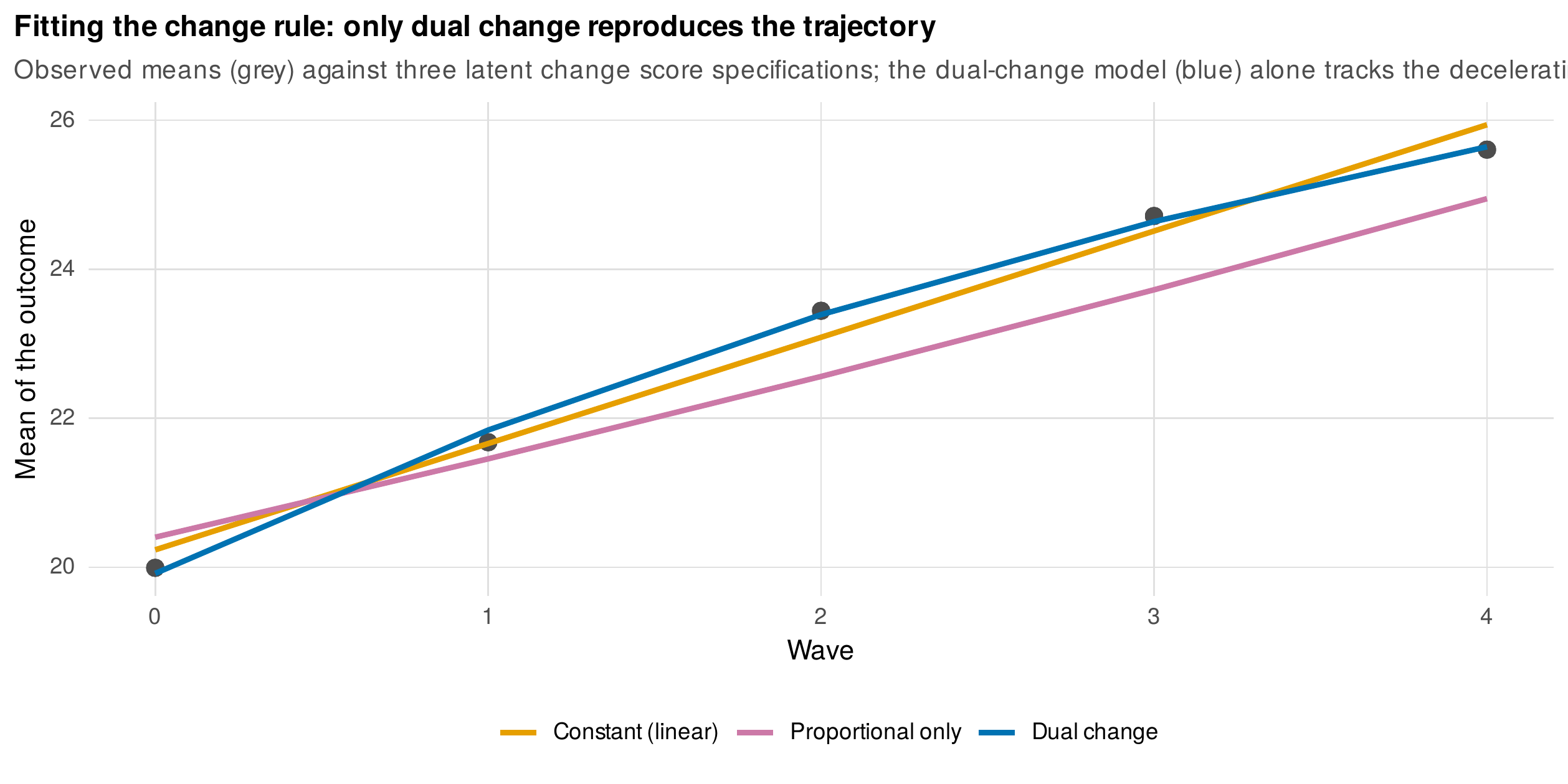
Note. Observed means (grey) of a decelerating process against the implied trajectories of three latent change score specifications. The constant-change and proportional-only models miss the shape; the dual-change model, which combines a constant increment with a proportional pull toward an asymptote, tracks it. The information criteria prefer the dual-change model decisively.
Table 20.2. A glossary of latent change score parameters.
| Parameter | Interpretation |
|---|---|
| Constant change mean | The average additive increment per interval, the linear part of change |
| Constant change variance | Individual differences in the additive increment |
| Proportional coefficient | The part of each change that is a proportion of the current level; its sign sets approach or acceleration |
| Initial true score mean and variance | The average and spread of the starting level |
| Initial-change covariance | Whether those who start higher change differently |
Note. The constant-change parameters describe the linear part of change and the proportional coefficient the state-dependent part. The proportional coefficient carries the model’s dynamic content and is the parameter most in need of the interpretive care developed below.
Table 20.3. Parameter configurations and the dynamics they imply.
| Configuration | Shape | Reading |
|---|---|---|
| Constant \(> 0\), proportional \(= 0\) | Linear | Steady change, no self-feedback |
| Constant \(= 0\), proportional \(< 0\) | Decay | Return toward zero (regulation) |
| Constant \(> 0\), proportional \(< 0\) | Asymptotic | Approach to a nonzero equilibrium |
| Proportional \(> 0\) | Accelerating | Self-amplifying change |
Note. The sign of the proportional coefficient distinguishes self-regulating dynamics, which pull the process back toward an equilibrium, from self-amplifying dynamics, which push it away. This dynamic reading is the change score model’s distinctive contribution.
The proportional coefficient carries a caution that debuts here and dominates the continuous-time chapter. It is defined per observation interval: a coefficient of \(-0.2\) means that a fifth of the gap to the asymptote closes between adjacent measured occasions, and if the occasions were twice as far apart the coefficient would be different, because more closing happens over a longer interval. Figure 20.4 demonstrates this by refitting the same process sampled at every wave and at every other wave: the proportional coefficient changes substantially, from about \(-0.2\) to about \(-0.4\), not because the process changed but because the interval did. This interval dependence means that proportional coefficients from studies with different measurement schedules are not comparable, and it is the single strongest argument for the continuous-time reparameterization of Chapter 27, in which the rate is a property of the process rather than of the sampling.
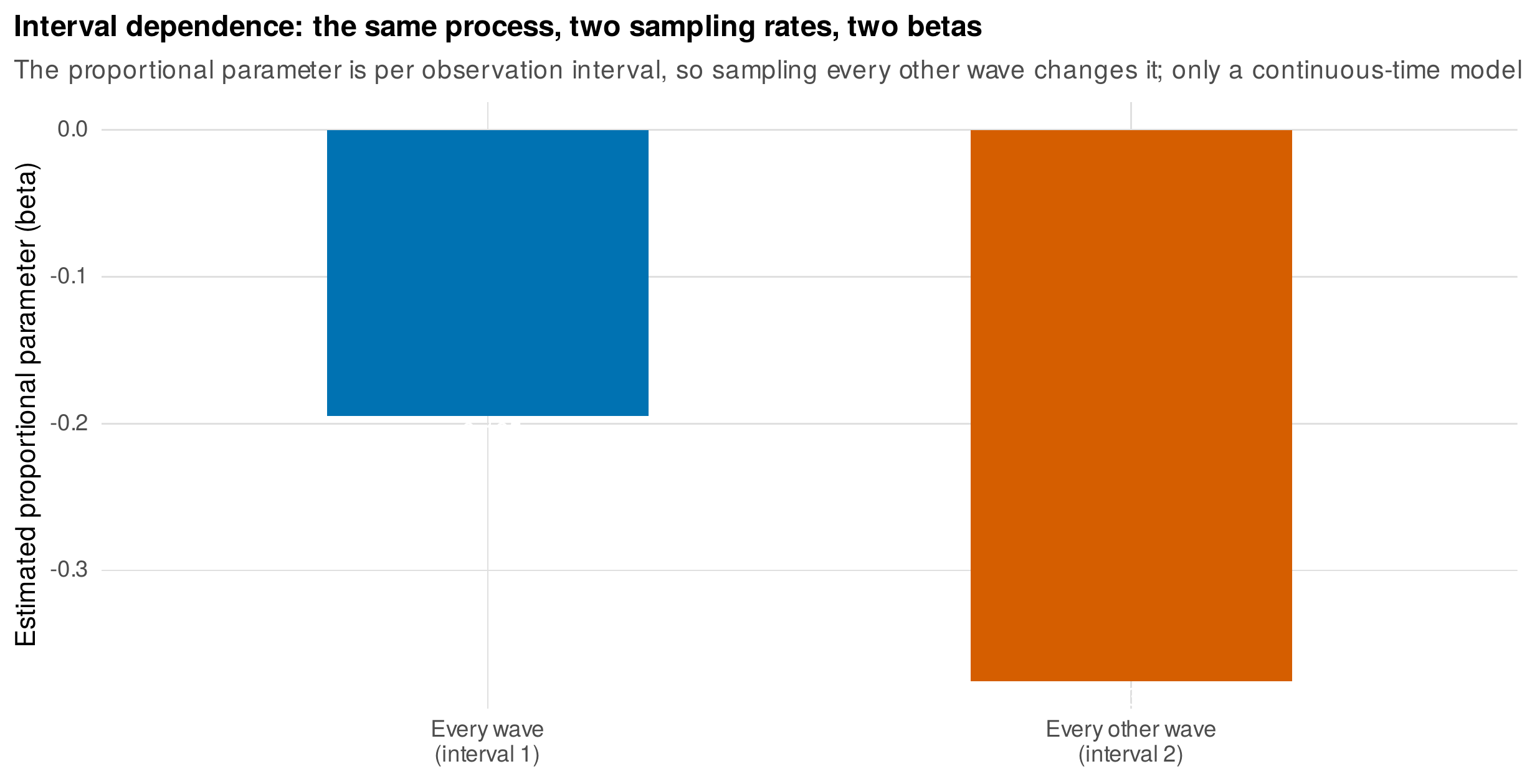
Note. The estimated proportional coefficient for the same process, sampled at every occasion and at every second occasion. The coefficient nearly doubles in magnitude, not because the dynamics changed but because the interval did. Discrete proportional coefficients are per-interval quantities and are not comparable across studies with different schedules; only a continuous-time rate is.
20.3 Bivariate Change Score Models and Coupling
The extension that draws the most interest, and the most trouble, couples two change score systems so that the level of one process drives the change in the other. Figure 20.5 sketches the architecture: two dual-change systems side by side, with coupling paths carrying the true score of each process at one occasion into the change of the other at the next. A positive coupling from a first process to the change of a second means that being higher on the first predicts subsequent increase in the second, the structural expression of the claim that the first process leads the second. On the running data, generated with an asymmetric coupling in which one process drives the other but not the reverse, the bivariate model recovers exactly that: a substantial coupling in the generating direction and a negligible one in the other, correctly identifying the lead-lag structure. The temptation is to read such a result as settling the causal question, and the temptation must be resisted.
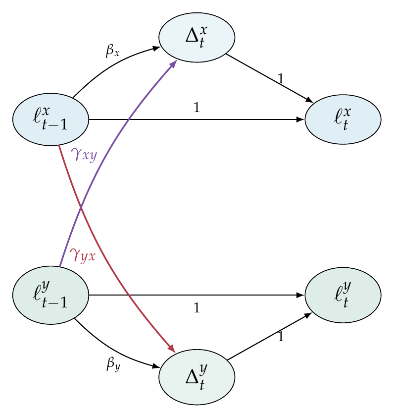
Note. Two dual-change systems, for processes \(x\) (top) and \(y\) (bottom), each with its own proportional self-feedback. The coupling paths carry the level of one process at the previous occasion into the change of the other: \(\gamma_{yx}\) (red) is the effect of \(x\)’s level on \(y\)’s change, and \(\gamma_{xy}\) (purple) the reverse. Asymmetry in the couplings is the structural expression of a lead-lag claim.
The interpretation of a coupling parameter demands a numbered discipline, because the coupling literature has repeatedly over-claimed. First, the coupling is conditional on the entire system, so its value and even its sign can change when another path is added or removed, which mandates a drop-one sensitivity analysis. Second, it is interval-dependent, inheriting the problem of the proportional coefficient. Third, the coupling absorbs measurement error unless the model separates true score from error, which is an argument for the second-order variant. Fourth, the meaning of a coupling depends on the self-feedback coefficients alongside it, because a level effect reads differently against a self-regulating than a self-amplifying process. Fifth, some bivariate change score models are statistically equivalent to constrained cross-lagged panel models, so a coupling result may have an equivalent-model shadow that a different but equally fitting specification would describe in other terms, the unification that Chapter 21 develops. The book’s standard, in response, is a sensitivity battery: refit the coupling under a range of defensible specifications and report the stability of the estimate, not a single point. Figure 20.6 shows the battery on the running coupling, whose estimate is reassuringly stable across specifications, and Table 20.4 is the checklist. A coupling that survives the battery earns a cautious lead-lag reading; one that does not is an artifact of a particular specification.
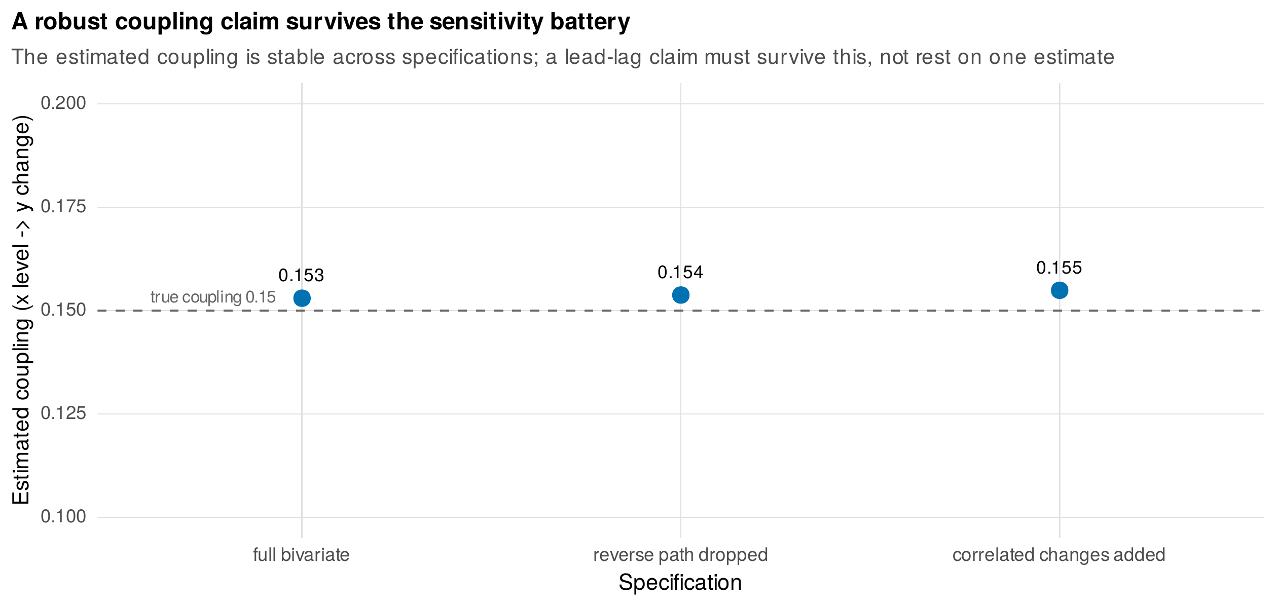
Note. The estimated coupling under alternative specifications, against its true value. The estimate is stable, which is what licenses a cautious lead-lag reading. A coupling that moved substantially across these specifications would be an artifact of the chosen model, not a finding, and reporting only a single point estimate hides that risk.
Table 20.4. A sensitivity battery for a coupling claim.
| Check | What it guards against |
|---|---|
| Drop each other path in turn | Coupling conditional on the whole system |
| Vary the interval or note it | Interval dependence of the estimate |
| Fit a second-order (error-free) variant | Measurement error absorbed into coupling |
| Compare to a cross-lagged specification | Equivalent-model shadow |
| Report the estimate across all of these | A single point estimate hiding instability |
Note. A lead-lag claim from a bivariate change score model is credible only if it is stable across this battery. The book’s position is that the coupling literature has over-claimed by reporting point estimates from single specifications; the remedy is to raise the evidentiary bar to demonstrated stability.
The coupling system is a set of difference equations, and reading it as such previews Part VI. The pair of change rules defines, at every combination of the two levels, an expected one-step change in each, and plotting these as arrows gives a vector field, the discrete-time image of a dynamical system’s flow. Figure 20.7 draws it for the fitted coupled system: the arrows show the process flowing from wherever it starts toward an equilibrium, and the shape of the flow, whether it spirals, converges directly, or diverges, is the qualitative dynamics that the parameters encode. This is precisely the picture that the vector autoregressive and continuous-time models of Part VI will formalize, and drawing it here makes the change score model the bridge it is.
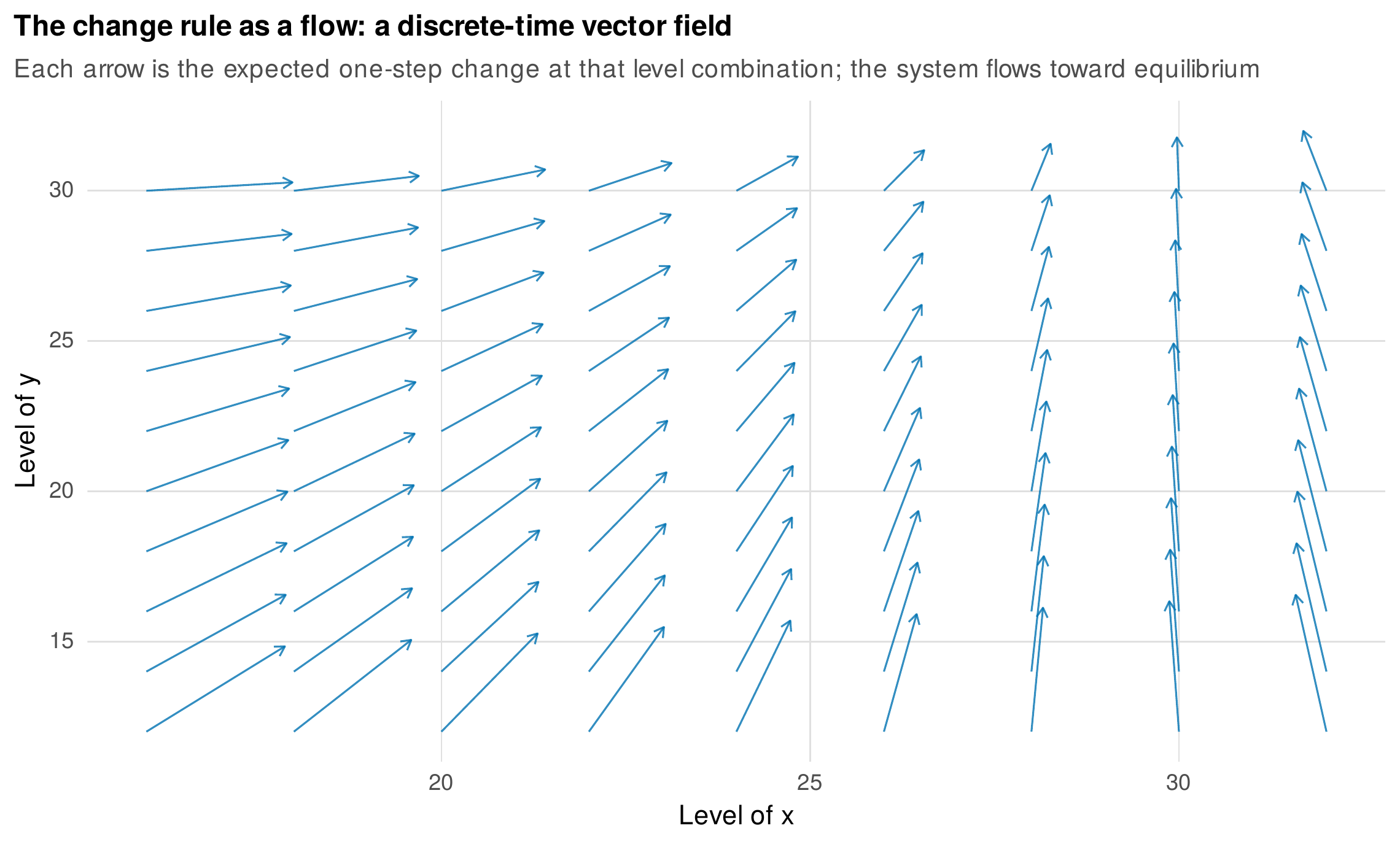
Note. Each arrow is the expected one-step change in the two processes at that combination of their levels, from the fitted coupled model. The field shows the system flowing toward its equilibrium. This dynamical-systems reading of a change score model is the bridge to the vector autoregressive and continuous-time models of Part VI.
20.4 Second-Order Growth Models
The measurement invariance of Chapter 18 was established so that its check could be cashed here. A second-order growth model places the growth structure not on observed scores or composites but on the latent construct measured by multiple indicators: a first-order measurement model, with invariant loadings and intercepts, defines a factor at each occasion, and a second-order growth model fits an intercept and slope to those factors. The construction requires the invariance chain, with scalar invariance necessary for the factor means to be comparable and hence for growth in the factor mean to be meaningful, and Table 20.5 states which level licenses what. The payoff is twofold: the growth is fitted to an error-free construct, so measurement error no longer attenuates it, and the invariance is testable rather than assumed. Figure 20.8 shows the payoff on the engagement data of Chapter 18, whose second indicator drifted: the second-order model, fitting growth to the partially invariant latent construct, recovers the true slope, while the composite score, which silently assumes strict invariance, overstates it, the real-data echo of the consequences simulation of Chapter 18. Fitting growth to a composite is fitting it to a measure whose meaning may have shifted; fitting it to an invariant factor is fitting it to the construct. Two multivariate second-order forms exist and answer different questions, the curve-of-factors model, which fits one growth process to a factor measured at each wave, and the factor-of-curves model, which fits a higher-order factor to several separate growth processes, and the choice between them follows the substantive structure of the constructs.
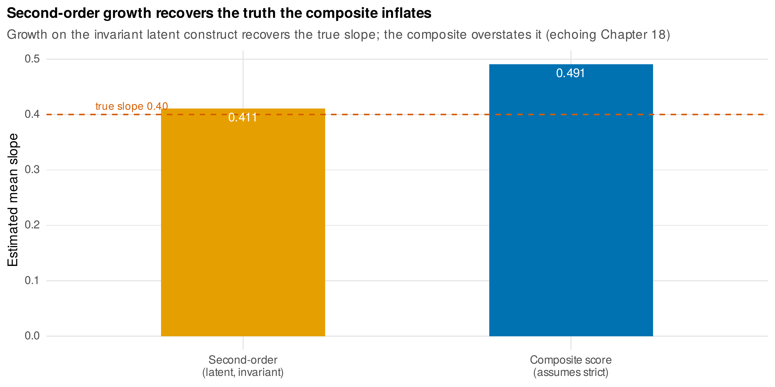
Note. The estimated mean slope of the engagement construct from a second-order growth model on the invariant latent factors and from a growth model on the composite score, against the true slope. The second-order model recovers the truth; the composite, silently assuming strict invariance that the drifting item violates, overstates the growth. The measurement check of Chapter 18 has real consequences for the estimated rate of change.
Table 20.5. The invariance requirements for a second-order growth model.
| Invariance level required | What it licenses in the growth model |
|---|---|
| Configural | The same construct is measured at each wave |
| Metric (loadings) | The factor variances and covariances are comparable across waves |
| Scalar (intercepts) | The factor means are comparable, so growth in the mean is meaningful |
| Partial scalar | Growth in the mean with a justified anchor set when some items drift |
Note. Growth in the latent mean requires at least partial scalar invariance, because without it a change in the factor mean confounds construct change with measurement drift. The second-order growth model makes the invariance testable rather than assuming it, as a composite silently does.
20.5 Structured Nonlinear Growth
Beyond the change score and second-order models lies a family of structured latent curve models that impose a specific nonlinear target function, an exponential, a logistic, a spline, through constrained loadings derived from the function’s form (Blozis, 2004). These give the interpretive precision of a named functional form with the flexibility of the latent-variable framework, and they occupy the ground between the freed-loading latent basis of Chapter 19, which imposes no shape, and the fully parametric nonlinear mixed models of Chapter 14, which impose a rigid one. This chapter treats them as a map rather than a residence: when a theory specifies a particular curve with interpretable parameters, a structured latent curve or a nonlinear mixed model fits it; when the shape is unknown, the latent basis estimates it; and when the individually varying times or the multilevel nesting that the structural equation framework handles awkwardly dominate, the mixed-model and additive approaches of Chapters 14 and 30 are the better home. The point is that the frameworks form a continuum of assumptions about the shape of change, from none to a fully specified function, and the analyst chooses the position on that continuum that the theory and the data warrant.
20.6 Running Change Score Models in R
Writing latent change score syntax by hand is error-prone beyond a few waves, so the shipped analysis provides a generator that produces the lavaan syntax from a variable name and a wave count, a companion artifact the reader can reuse and extend.
library(lavaan)
# lcs_syntax(v, W, dual, prop) builds the univariate model (see ch20_analysis_V01.R)
dual  <- sem(lcs_syntax("x", W = 5, dual = TRUE,  prop = TRUE),  data = d)   # dual change
const <- sem(lcs_syntax("x", W = 5, dual = TRUE,  prop = FALSE), data = d)   # constant only
anova(const, dual)                                                            # compare specifications
The bivariate generator combines two univariate systems and adds the coupling paths, and the second-order growth model puts the intercept and slope factors on the invariant wave factors of Chapter 18.
# bivariate coupling: the level of one process predicts the change of the other
biv <- sem(lcs_bivariate(W = 5, coupling = "both"), data = d)
# second-order growth: growth factors on latent constructs (invariant measurement)
# I =~ 1*f1 + 1*f2 + 1*f3 + 1*f4 ; S =~ 0*f1 + 1*f2 + 2*f3 + 3*f4
The complete analysis, including the specification ladder, the interval-dependence demonstration, the bivariate coupling with its sensitivity battery, the implied vector field, and the second-order growth comparison with the composite, is the shipped script ch20_analysis_V01.R, with figures drawn by ch20_figures_V01.R and the dataset generated by gen_lcs_V01.R.
Software Note • change score models across programs
Latent change score models are fitted in lavaan, in Mplus through its MODEL syntax with the change scores defined by fixed paths, and in OpenMx, which offers the most flexibility for the many equality constraints and for the definition variables that individually varying intervals require. The non-positive-definite latent covariance warnings that these models routinely produce are usually benign, a consequence of the change scores being deterministic functions of the true scores rather than a sign of misspecification, and should be checked rather than feared. For serious dynamic modeling with unequal intervals the continuous-time tools of Chapter 27, the ctsem package foremost, supersede the discrete change score model by estimating an interval-free rate, and the relation between the two parameterizations is exact (Voelkle & Oud, 2015).
20.7 Common Misconceptions
Several beliefs about change score models mislead. The first is that a change score model is just a growth model with extra steps; it makes a different scientific claim, about the rule generating change rather than the shape of the trajectory, and the two can be distinguished by data that a rule fits and a shape does not. The second is that a negative proportional coefficient is a regression-to-the-mean artifact; it can be an artifact of measurement error, which the second-order variant removes, but it can equally be genuine self-regulation, and the two are separated by modeling, not assumed. The third is that a bivariate change score model settles causal direction; the sensitivity battery exists precisely because it does not, and a coupling is credible only when stable across specifications. The fourth is that second-order models are for psychometric purists; the evidence on bias and power says they matter for anyone estimating change in a latent construct. The fifth is that a proportional coefficient can be compared across studies; it is interval-dependent and cannot, absent a continuous-time reparameterization.
Common Pitfall • four errors in change score practice
First, hand-writing the syntax: beyond a few waves the fixed-path scaffolding is transcription-error-prone, so use a generator. Second, reading a coupling as Granger-style causality: a level-to-change path is not a settled causal direction, and the sensitivity battery is mandatory. Third, comparing proportional coefficients across schedules: they are per-interval and not comparable; move to continuous time. Fourth, fitting second-order growth without scalar invariance: growth in a latent mean requires at least partial scalar invariance, or it confounds construct change with measurement drift.
Chapter Summary
The latent change score model treats change between adjacent true scores as a modeled latent variable, built from a scaffolding of fixed unit paths that enforce the identity of change as a difference, with the free parameters on the change: a constant increment and a proportional coefficient (Figure 20.1). The change rule generates a family of trajectory shapes, linear, decaying, asymptotic, and accelerating, the same curves the nonlinear mixed models of Chapter 14 trace directly (Figure 20.2, Table 20.1), and fitting the specification ladder recovers the generating rule (Figure 20.3, Tables 20.2 and 20.3). The proportional coefficient is per observation interval and not comparable across schedules, the strongest argument for continuous time (Figure 20.4). Coupling two systems expresses lead-lag structure through level-to-change paths (Figure 20.5), but a coupling claim requires a sensitivity battery, because the parameter is conditional, interval-dependent, error-absorbing, and shadowed by equivalent models (Figure 20.6, Table 20.4); read as difference equations, the coupled system is a discrete-time vector field, the bridge to Part VI (Figure 20.7). The second-order growth model cashes the invariance check of Chapter 18 by fitting growth to an error-free latent construct, recovering the truth a composite inflates (Figure 20.8, Table 20.5), and the structured latent curve models complete a continuum of assumptions about the shape of change.
Where to Go Next
This chapter turns the corner from describing change to modeling its dynamics, and the corner opens onto the rest of the book. Chapter 21 shows the latent change score model, the cross-lagged panel model, and the random-intercept panel models to be members of one unified family, resolving the equivalent-model shadow that the coupling section raised, and it is the natural next step for anyone who has met coupling here. Chapter 27 resolves the interval-dependence problem by estimating a continuous-time rate that is a property of the process rather than of the sampling schedule, and it makes the difference-equation reading of this chapter literal. The vector-field picture of the coupled system is the discrete preview of the vector autoregressive and dynamic structural equation models of Chapters 24 and 25, which model the same flow within persons over intensive measurements. The second-order growth model completes the measurement-first chain begun in Chapter 18, and the developmental-cascade applications of Chapter 34 deploy the bivariate coupling machinery on substantive questions of how one domain of development pulls another along.
Exercises
- 20.1 Derive the trajectory. For a four-wave dual-change model with given constant-change and proportional parameters, compute the implied means by unrolling the recurrence, and verify them against a
lavaanfit. - 20.2 Fit the ladder. On a provided dataset, fit the constant, proportional, and dual-change models, compare them, and write a defensible conclusion about the change rule.
- 20.3 Interval-dependence lab. Simulate a dual-change process, refit it on every occasion and on every second occasion, and show that the proportional coefficient changes while the trajectory does not.
- 20.4 Coupling sensitivity. On bivariate data, estimate the coupling and run the full sensitivity battery, then write the caveated lead-lag conclusion the battery supports.
- 20.5 Second-order growth. Build a second-order growth model from an invariant measurement model and compare its slope inference to a composite-based growth model, interpreting the difference.
- 20.6 Use the generator. Read the shipped syntax generator, use it to fit a five-wave model, and extend it with one new option.
References
Blozis, S. A. (2004). Structured latent curve models for the study of change in multivariate repeated measures. Psychological Methods, 9(3), 334–353. https://doi.org/10.1037/1082-989X.9.3.334
Ferrer, E., Balluerka, N., & Widaman, K. F. (2008). Factorial invariance and the specification of second-order latent growth models. Methodology, 4(1), 22–36. https://doi.org/10.1027/1614-2241.4.1.22
Ferrer, E., & McArdle, J. J. (2003). Alternative structural models for multivariate longitudinal data analysis. Structural Equation Modeling, 10(4), 493–524. https://doi.org/10.1207/S15328007SEM1004_1
Ferrer, E., & McArdle, J. J. (2010). Longitudinal modeling of developmental changes in psychological research. Current Directions in Psychological Science, 19(3), 149–154. https://doi.org/10.1177/0963721410370300
Grimm, K. J., An, Y., McArdle, J. J., Zonderman, A. B., & Resnick, S. M. (2012). Recent changes leading to subsequent changes: Extensions of multivariate latent difference score models. Structural Equation Modeling, 19(2), 268–292. https://doi.org/10.1080/10705511.2012.659627
Grimm, K. J., Ram, N., & Estabrook, R. (2017). Growth modeling: Structural equation and multilevel modeling approaches. Guilford Press.
Hamagami, F., & McArdle, J. J. (2007). Dynamic extensions of latent difference score models. In S. M. Boker & M. J. Wenger (Eds.), Data analytic techniques for dynamical systems (pp. 47–85). Lawrence Erlbaum Associates.
Hancock, G. R., Kuo, W.-L., & Lawrence, F. R. (2001). An illustration of second-order latent growth models. Structural Equation Modeling, 8(3), 470–489. https://doi.org/10.1207/S15328007SEM0803_7
Kievit, R. A., Brandmaier, A. M., Ziegler, G., van Harmelen, A.-L., de Mooij, S. M. M., Moutoussis, M., Goodyer, I. M., Bullmore, E., Jones, P. B., Fonagy, P., Lindenberger, U., & Dolan, R. J. (2018). Developmental cognitive neuroscience using latent change score models: A tutorial and applications. Developmental Cognitive Neuroscience, 33, 99–117. https://doi.org/10.1016/j.dcn.2017.11.007
McArdle, J. J. (2009). Latent variable modeling of differences and changes with longitudinal data. Annual Review of Psychology, 60(1), 577–605. https://doi.org/10.1146/annurev.psych.60.110707.163612
McArdle, J. J., & Hamagami, F. (2001). Latent difference score structural models for linear dynamic analyses with incomplete longitudinal data. In L. M. Collins & A. G. Sayer (Eds.), New methods for the analysis of change (pp. 139–175). American Psychological Association. https://doi.org/10.1037/10409-005
McArdle, J. J., & Nesselroade, J. R. (2014). Longitudinal data analysis using structural equation models. American Psychological Association. https://doi.org/10.1037/14440-000
Rosseel, Y. (2012). lavaan: An R package for structural equation modeling. Journal of Statistical Software, 48(2), 1–36. https://doi.org/10.18637/jss.v048.i02
Usami, S., Murayama, K., & Hamaker, E. L. (2019). A unified framework of longitudinal models to examine reciprocal relations. Psychological Methods, 24(5), 637–657. https://doi.org/10.1037/met0000210
Voelkle, M. C., & Oud, J. H. L. (2015). Relating latent change score and continuous time models. Structural Equation Modeling, 22(3), 366–381. https://doi.org/10.1080/10705511.2014.935918