Chapter 21
Cross-Lagged Panel Designs: CLPM, RI-CLPM, and Causal Inference with Panel Data
Few questions in psychology are asked more often than whether one thing leads to another over time: whether self-esteem drives later depression or the reverse, whether engagement raises later achievement, whether media use fuels later aggression. For half a century the reflexive tool for such questions was the cross-lagged panel model, in which each variable predicts the other at the next wave while its own stability is held constant, and a significant cross-lag was read as a prospective effect. This chapter is the book’s reckoning with that tool. It shows, algebraically and by a fully coded simulation, that when people differ in stable ways the classic model conflates those stable differences with the carrying-forward of states, so that its cross-lags can be inflated, attenuated, or invented outright. It then develops the random intercept cross-lagged panel model that separates the stable between-person layer from the within-person dynamics, places both models inside a larger family whose members encode different assumptions about traits, growth, and dynamics, and insists that the choice among them is a choice of estimand rather than of fashion. The fairness burden here is unusual: the repair has its own critics, and their arguments, that within-person effects are short-run and occasion-specific and that the between-person question is sometimes the right one, are given full voice. The chapter closes on what panel data can and cannot license as a causal claim, using directed acyclic graphs and a fixed-effects bridge, and on longitudinal mediation, where cross-sectional shortcuts mislead.
Learning Objectives
After working through this chapter, you should be able to: (1) specify the classic cross-lagged panel model and state precisely why its cross-lags blend within- and between-person information when stable trait variance is present; (2) specify the random intercept cross-lagged panel model, interpret its parameters as within-person quantities, and state its identification and wave requirements; (3) place the CLPM, RI-CLPM, autoregressive latent trajectory model, latent curve model with structured residuals, general cross-lagged panel model, and bivariate latent change score model in a unified framework and choose among them by estimand; (4) apply directed acyclic graph reasoning to panel designs and state what person-level fixed effects do and do not remove; (5) reconcile an econometric fixed-effects estimate with the RI-CLPM within-person effects; (6) analyze longitudinal mediation with Monte Carlo confidence intervals and explain why cross-sectional mediation is biased; and (7) conduct and report the model-comparison and sensitivity workflow that a directional claim requires.
21.1 The Reciprocal-Causation Question and the Classic Model
The question that motivates this chapter is reciprocal influence over time. Does a person’s self-esteem shape their later depressive symptoms, or do symptoms erode later self-esteem, or both? Does students’ engagement raise their later achievement, or does success feed later engagement? These are questions about temporal precedence, about which of two intertwined processes moves first, and panel data, the same persons measured on both variables at several occasions, seem tailor-made to answer them. The classic tool is the cross-lagged panel model (CLPM), a structural equation model in which each variable at each wave is regressed on both variables at the previous wave. The regression of a variable on its own past is an autoregression, read as stability or carryover; the regression of a variable on the other variable’s past is a cross-lagged effect, and it is the object of interest. The traditional reading is seductive in its simplicity: the cross-lag from \(x\) to \(y\) is the prospective effect of \(x\) on later \(y\) after controlling for the stability of \(y\), and if it is significant while the reverse cross-lag is not, \(x\) leads \(y\).
Figure 21.1, upper panel, draws the model for three waves. The autoregressive coefficients \(a\) and \(d\) run along each variable’s own chain, the cross-lags \(b\) and \(c\) run diagonally between the chains, and the curved paths are the covariance of the two variables at the first wave and the covariances of their residuals at later waves, which capture contemporaneous association not explained by the lagged structure. In the constrained version used throughout this chapter, the four dynamic coefficients are held equal across waves, an assumption of stationarity that buys interpretability and power and that should itself be tested. The model is fitted by maximum likelihood in any structural equation program, and with more than two waves it is overidentified, so it has a testable fit.
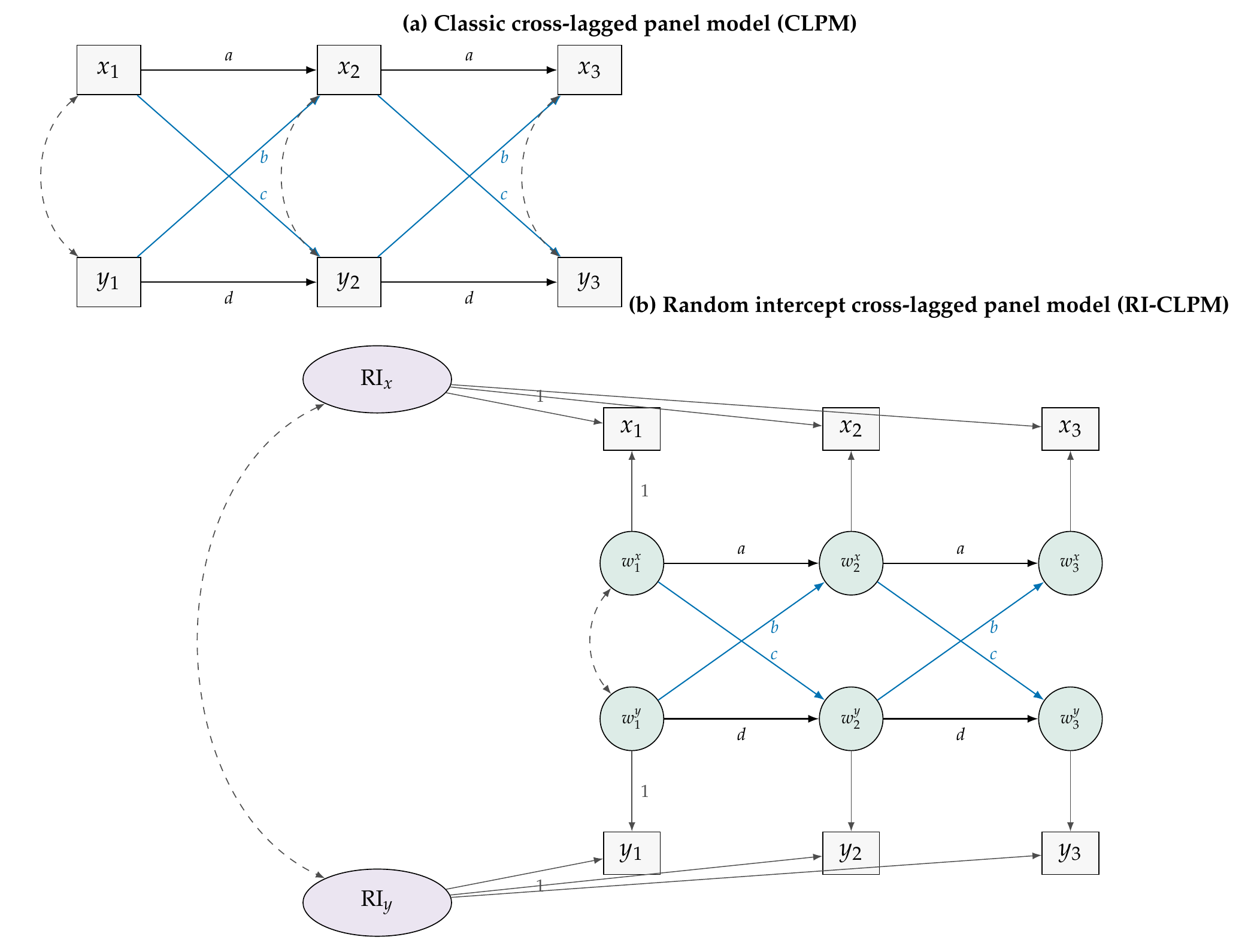
Note. Rectangles are observed scores, circles are within-person components, ellipses are stable trait random intercepts. In the CLPM (a) the lagged structure operates directly on the observed scores, so a person’s stable elevation is carried by the autoregressions. In the RI-CLPM (b) each observed score is the sum of a trait random intercept (loading one) and a within-person component (loading one); the autoregressions \(a,d\) and cross-lags \(b,c\) operate only on the within-person components, and the trait covariance (left) absorbs the stable between-person association. The blue diagonals are the cross-lags of interest.
The technique has a long lineage. Its ancestor is the cross-lagged panel correlation of the 1960s, which compared the two cross-lagged correlations \(r(x_1,y_2)\) and \(r(y_1,x_2)\) and inferred causal predominance from their difference. Rogosa (1980) dismantled that comparison, showing that the two cross-lagged correlations depend on the variables’ different reliabilities and stabilities and can differ even when neither variable causes the other, so that the correlational version identifies nothing. The structural equation version, which regresses rather than correlates and thereby holds stability constant, was widely believed to have repaired the problem, and for three decades the CLPM was the developmental and personality psychologist’s default. The critique that reopened the question, and that organizes this chapter, is more subtle than Rogosa’s and took the field by surprise.
21.2 The Critique, Made Rigorous
The modern critique, stated most influentially by Hamaker, Kuiper, and Grasman (2015), is that the CLPM omits a layer of structure that is almost always present in psychological data: stable, trait-like differences between persons that persist across all waves. People differ in their characteristic level of self-esteem, their typical engagement, their baseline symptom load, and these differences are not the same thing as the wave-to-wave carrying-forward of a state. The CLPM has only one mechanism, the autoregression, to represent all persistence, so it forces the stable trait and the dynamic carryover through the same coefficient. When a stable trait is present, the autoregression is inflated because it must reproduce the high correlation between a person’s scores at distant waves that the trait induces, and, more damagingly, the cross-lags are contaminated. If the two traits are correlated across persons, which they usually are (people high in trait \(x\) tend to be high in trait \(y\)), the CLPM has no parameter for that between-person association except the cross-lags, and it presses them into service, reporting a prospective effect where there is only a stable correlation.
21.2.1 The Within-Between Confound in Dynamic Clothing
This is the same confound that runs through the whole book, the conflation of within-person and between-person information that Chapter 1 introduced with Lord’s paradox and that Chapter 13 addressed by centering predictors, the connection between centering and the fixed-versus-random-effects choice being made explicit by Hamaker and Muthén (2020). Here it wears dynamic clothing. A between-person association, that people who are more engaged than others also achieve more than others, is a statement about the ranking of persons and says nothing about process. A within-person effect, that a student who is more engaged than usual for them goes on to achieve more than usual for them, is a statement about how one person’s deviations propagate over time, and it is what a causal claim about engagement requires. The CLPM’s cross-lag mixes the two, and the mixture is dominated by the between-person part whenever the stable trait accounts for a large share of the variance, which Figure 21.2 shows is the norm rather than the exception.
Foundations Box • The algebra of cross-lag bias under an omitted trait
Write the observed score as the sum of a stable trait and a within-person part, \(x_{it}=\mu^x_i+w^x_{it}\) and \(y_{it}=\mu^y_i+w^y_{it}\), where the traits \((\mu^x_i,\mu^y_i)\) are fixed for a person across waves and correlated across persons with covariance \(\sigma_{\mu}\). Suppose the true within-person dynamics contain no effect of \(x\) on \(y\), so that \(w^y_{it}\) does not depend on \(w^x_{i,t-1}\). The CLPM regresses \(y_{it}\) on \(x_{i,t-1}\) and \(y_{i,t-1}\) on the observed scores, which still carry the traits. Because \(x_{i,t-1}\) contains \(\mu^x_i\), which is correlated with \(\mu^y_i\), which is contained in \(y_{it}\), the regression of \(y_{it}\) on \(x_{i,t-1}\) has a nonzero population coefficient even after conditioning on \(y_{i,t-1}\): the single lagged control \(y_{i,t-1}\) is one fallible measurement of the trait \(\mu^y_i\) and cannot fully absorb it. The residual trait covariance leaks into the cross-lag, whose probability limit is a positive multiple of \(\sigma_{\mu}\) even though the within-person effect is zero. The random intercept, which is a latent common factor for a person’s scores across all waves, removes \(\mu^y_i\) exactly rather than through a single noisy proxy, and the leak closes.
21.2.2 The Signature Simulation
The clearest way to see the problem is to build data in which the truth is known and watch the CLPM miss it. The shipped dataset panel_sim contains \(1{,}000\) persons measured on two variables at five waves, generated from a model with stable person traits and a within-person dynamic system. The within-person truth is deliberately asymmetric: the effect of \(x\) on later \(y\) is \(0.20\), so \(x\) genuinely leads \(y\), while the effect of \(y\) on later \(x\) is exactly zero. Both within-person autoregressions are \(0.40\). On top of this dynamic system sit two stable traits, correlated at \(0.60\) across persons, that account for a little over forty percent of each variable’s observed variance (Figure 21.2). Every parameter is visible in the generating script gen_panel_sim_V01.R, so nothing about the comparison is hidden.
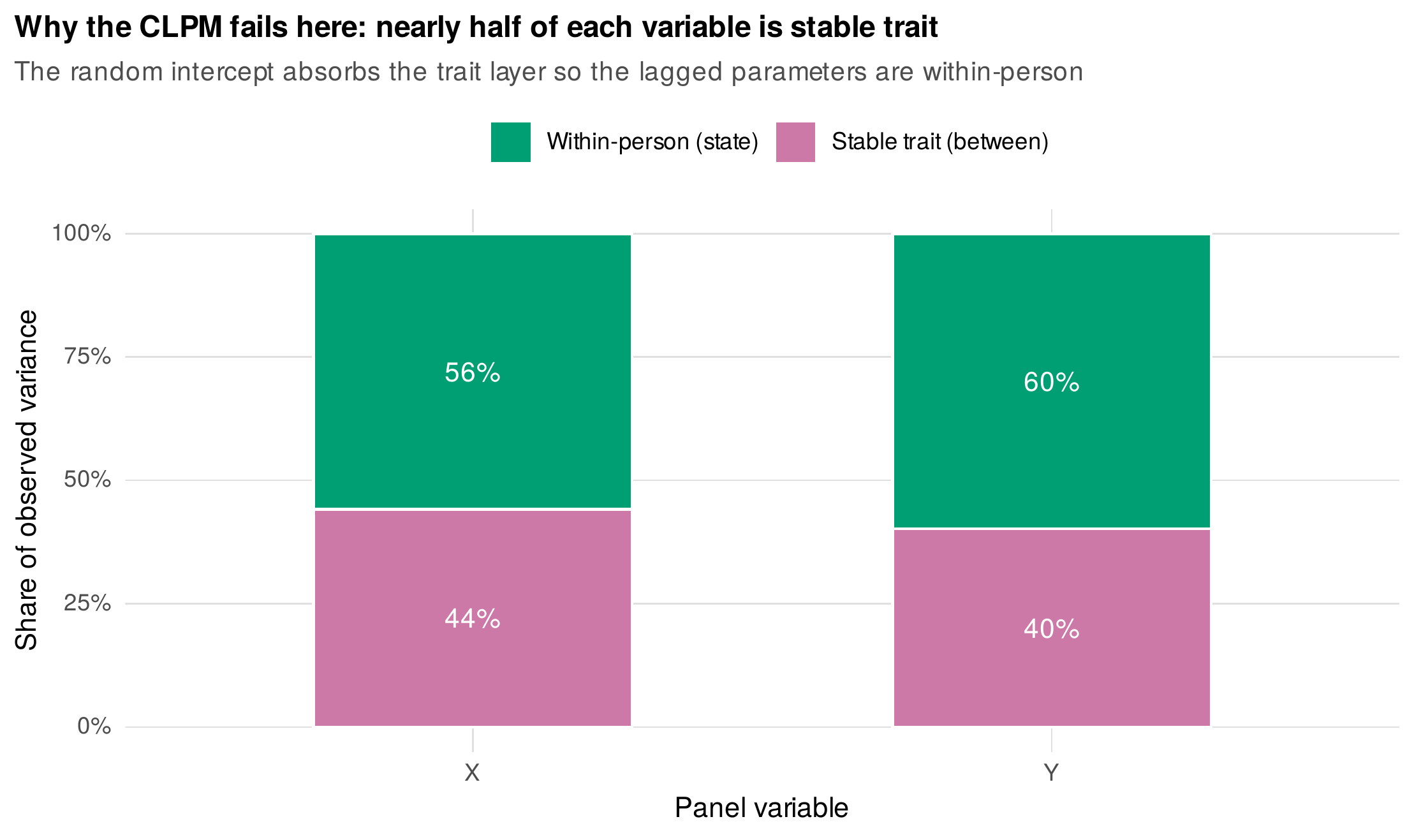
Note. Each panel variable is decomposed into the share of observed variance that is stable trait (between-person) and the share that is within-person state, as recovered by the RI-CLPM. Roughly two fifths of each variable is stable trait. This is the regime in which the CLPM’s single autoregression cannot separate stable elevation from dynamic carryover, and the cross-lags absorb the difference.
Fitting both models to these data reproduces the critique exactly. Figure 21.3 is the chapter’s signature exhibit. The constrained CLPM estimates the two autoregressions at \(0.64\) and \(0.61\), far above their true value of \(0.40\), because they are absorbing the stable trait as well as the dynamic carryover. Worse, it reports the spurious \(y \to x\) cross-lag, whose true value is zero, as \(0.056\) with a standard error of \(0.012\) and \(p < .001\): a highly significant reciprocal effect that does not exist in the data-generating process. The genuine \(x \to y\) effect it estimates at \(0.187\), close by luck to the truth of \(0.20\) in this particular design, so that a researcher reading the CLPM output would conclude, wrongly, that the two variables influence each other reciprocally. The RI-CLPM, given exactly the same data, recovers the truth: autoregressions of \(0.41\) and \(0.43\), a \(y \to x\) effect of \(-0.014\) that is not significant (\(p = .49\)), and an \(x \to y\) effect of \(0.201\). It correctly reports a one-directional process. The RI-CLPM also fits the data better in the usual descriptive sense, with a root mean square error of approximation of \(0.021\) against the CLPM’s \(0.075\) and a comparative fit index of \(0.997\) against \(0.964\), but the fit difference is not the lesson. The lesson is that the two models answer different questions, and only the within-person question is the one the reciprocal-effects literature means to ask.
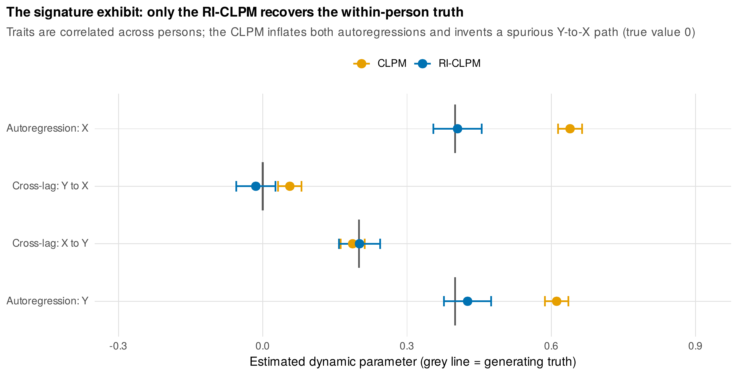
Note. Estimated dynamic parameters from the classic CLPM (orange) and the RI-CLPM (blue) fitted to panel_sim, with 95% confidence intervals; the grey vertical marks are the generating values. The CLPM inflates both autoregressions and reports a spurious, statistically significant \(y \to x\) cross-lag whose true value is zero. The RI-CLPM recovers all four within-person parameters.
A caution against overlearning from this exhibit is due immediately, and it anticipates the counter-current of Section 21.4. The CLPM did not fail because it is a bad model; it failed because its estimand, which blends between- and within-person information, is not the within-person estimand the simulation was built to test. In a world with no stable traits, the CLPM and RI-CLPM coincide. The critique is therefore conditional: it bites exactly to the degree that stable between-person differences are present, and its force is an empirical question about the data, answered by the variance decomposition of Figure 21.2, not a theorem that the RI-CLPM is always preferable.
21.3 The Random Intercept Cross-Lagged Panel Model
The repair proposed by Hamaker and colleagues (2015) and extended by Mulder and Hamaker (2021) adds one layer to the model. Each variable receives a random intercept, a latent factor that loads on that variable at every wave with a fixed loading of one, so that it represents the part of a person’s scores that is constant across all occasions, the stable trait. What is left after the random intercept is removed is a set of within-person components, one per variable per wave, each a latent variable with a fixed unit loading on its observed score, that represent a person’s temporary deviation from their own expected level at that occasion. Figure 21.1, lower panel, draws the structure: the observed score is the sum of the trait and the within-person component, and the entire autoregressive and cross-lagged machinery is moved off the observed scores and onto the within-person components. The two random intercepts are allowed to covary, and that covariance absorbs the stable between-person association that the CLPM had nowhere to put.
The reinterpretation this forces is the whole point. In the RI-CLPM the cross-lag from \(x\) to \(y\) is the effect of a person being above their own expected level on \(x\) at one occasion on their being above their own expected level on \(y\) at the next, a strictly within-person quantity purged of the ranking of persons. Table 21.1 sets the two readings side by side, parameter by parameter, because the words matter: the same Greek letter means a different thing in the two models, and reviewers and authors routinely carry the CLPM’s between-person gloss onto the RI-CLPM’s within-person coefficient, which is a category error.
Table 21.1. Parameter-by-parameter interpretation of the CLPM and the RI-CLPM.
| Quantity | CLPM reading | RI-CLPM reading |
|---|---|---|
| Autoregression | Rank-order stability plus dynamic carryover, blended | Within-person inertia: does a deviation from one’s own norm persist |
| Cross-lag \(x\to y\) | Prospective effect of \(x\)-level on later \(y\), controlling \(y\)-stability (blends within and between) | Effect of being above one’s own \(x\)-norm on later deviation from one’s own \(y\)-norm (within-person) |
| Stable individual differences | Not modeled; forced through autoregression and cross-lags | Captured by the random-intercept variances |
| Cross-construct trait link | Not modeled; leaks into cross-lags | Captured by the random-intercept covariance |
| Residual/innovation covariance | Contemporaneous association at each wave | Within-person co-movement of shocks |
Note. The two models attach different meanings to coefficients that look identical in output. Carrying the CLPM’s between-person language onto RI-CLPM estimates is a common and consequential error.
Identification and design requirements follow from the extra layer. Separating a stable trait from within-person dynamics requires at least three waves; with two waves the random intercept is not distinguishable from the wave-specific components, and the model reduces to a reparameterized CLPM that cannot deliver the promised separation. The wave-one within-person components are treated as predetermined, with freely estimated variances and covariance, because there is no earlier occasion to predict them; the lagged structure begins at the second wave. In the constrained form the four dynamic coefficients and the innovation (co)variances are held equal across the later waves, which requires and deserves a stationarity check. The model is fitted by maximum likelihood, and full-information maximum likelihood handles the missingness that dropout produces, exactly as in Chapters 19 and 20. The reusable generator shipped as part of ch21_analysis_V01.R writes the RI-CLPM lavaan syntax for any number of waves, so that the fixed unit loadings, the zeroed observed residual variances, and the orthogonality of the traits to the wave-one components are laid down without hand error.
# RI-CLPM skeleton (three waves; generator writes any number)
RIx =~ 1*x1 + 1*x2 + 1*x3        # stable trait for x
RIy =~ 1*y1 + 1*y2 + 1*y3        # stable trait for y
wx1 =~ 1*x1;  wx2 =~ 1*x2;  wx3 =~ 1*x3    # within components
wy1 =~ 1*y1;  wy2 =~ 1*y2;  wy3 =~ 1*y3
x1 ~~ 0*x1;  x2 ~~ 0*x2;  x3 ~~ 0*x3      # no leftover observed error
y1 ~~ 0*y1;  y2 ~~ 0*y2;  y3 ~~ 0*y3
wx2 ~ a*wx1 + b*wy1;  wx3 ~ a*wx2 + b*wy2  # within dynamics (constrained)
wy2 ~ c*wx1 + d*wy1;  wy3 ~ c*wx2 + d*wy2
RIx ~~ RIy;  RIx ~~ 0*wx1 + 0*wy1;  RIy ~~ 0*wx1 + 0*wy1
Two practical hazards recur. At low intra-class correlation, when the stable trait accounts for little variance, the random-intercept variance is estimated near zero and can go slightly negative, producing a Heywood case; the honest response is to report it, refit with the variance bounded at zero, and recognize that a near-zero trait variance is itself the finding that the CLPM and RI-CLPM will nearly agree. When intervals between waves are unequal, the constrained model is misspecified because a coefficient that means change per unit time cannot be constant across intervals of different length, an interval-dependence problem identical to the one Chapter 20 raised for the latent change score model and that Chapter 27 resolves with continuous-time estimation. These are gathered in the practice box below.
In Practice • Convergence and interval hazards in the RI-CLPM
When the trait variance is small, expect near-zero or slightly negative random-intercept variances; bound them at zero, report the intra-class correlations, and note that the two models will nearly coincide. When wave spacing is unequal, do not constrain the dynamics to equality across intervals of different length; either free the coefficients by interval or move to a continuous-time model (Chapter 27). Watch for non-convergence when waves are few and the within-person components carry little variance, and prefer full-information maximum likelihood to listwise deletion when dropout is present. Always confirm the group order and the parameter labels in the fitted object rather than assuming them, and inspect the standardized within-person estimates, since the unstandardized cross-lags are on the metric of the observed scores.
21.4 The Family and the Estimand Map
The CLPM and the RI-CLPM are two members of a larger family of panel models, unified by Usami, Murayama, and Hamaker (2019), that differ in what they assume about three things: whether there is a stable trait, whether there is systematic growth, and how the wave-to-wave dynamics are structured. Figure 21.4 sketches six members and Table 21.2 states each one’s assumption triple. The classic CLPM assumes no stable trait and no growth, only observed-score dynamics. The RI-CLPM adds a stable trait. The autoregressive latent trajectory model of Bollen and Curran (2004) adds a growth trajectory, an intercept and slope, and lets the residuals around it follow an autoregression, fusing the growth-curve and autoregressive traditions. The latent curve model with structured residuals of Curran, Howard, Bainter, Lane, and McGinley (2014) keeps a growth trajectory but moves the cross-lagged dynamics onto the residuals around it, which is often the cleaner separation of a developmental trend from within-person fluctuations. The general cross-lagged panel model of Zyphur and colleagues (2020a, 2020b) generalizes further, adding accumulating factors and letting shocks co-move, so that it can represent both short-run dynamics and long-run impulse responses. The bivariate latent change score model of Chapter 20 is the family member that writes the dynamics as change scores rather than as regressions, and it is close kin to the RI-CLPM when a trait is included.
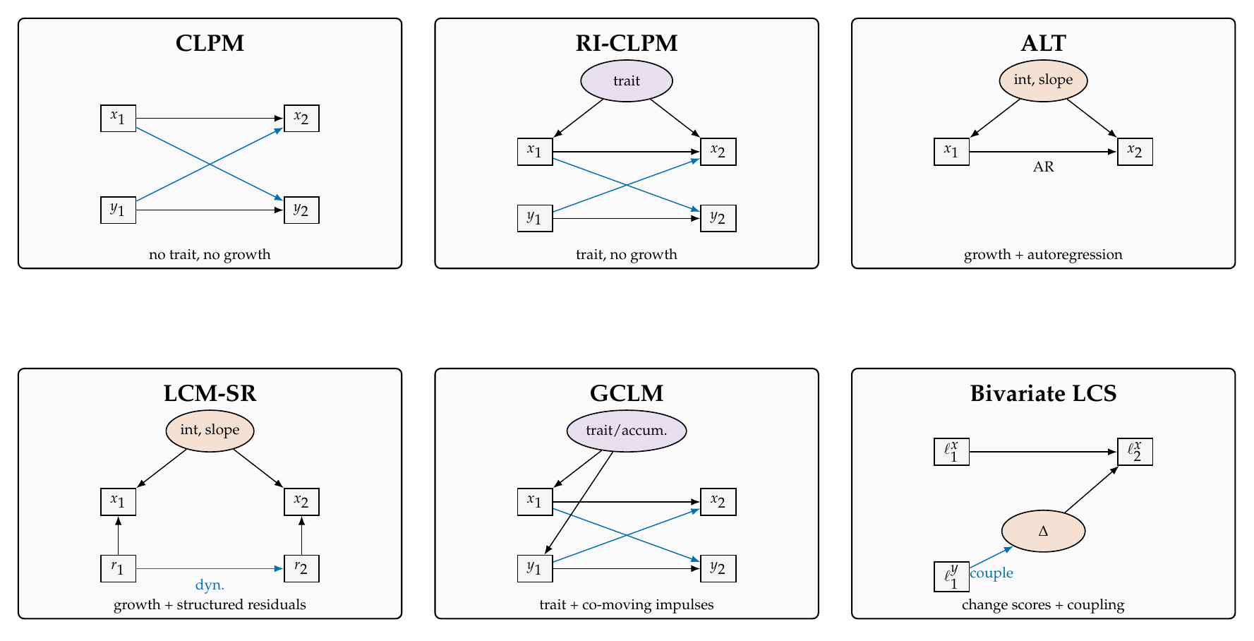
Note. Schematic glyphs, not full path diagrams: purple ellipses are stable traits or accumulating factors, orange ellipses are growth factors (intercept and slope), rectangles are observed scores, true scores, or residuals, and blue arrows are cross-lagged or coupling paths. Each member encodes a different assumption about trait, growth, and dynamics; Table 21.2 states the triples. The bivariate latent change score model of Chapter 20 is the change-score cousin of the RI-CLPM.
Table 21.2. The panel-model family and its assumptions.
| Model | Stable trait | Growth trend | Dynamics on | Estimand it answers |
|---|---|---|---|---|
| CLPM | No | No | Observed scores | Between-plus-within blend of prospective prediction |
| RI-CLPM | Yes (intercept) | No | Within components | Within-person carryover and cross-effects |
| ALT | Via trajectory | Yes | Observed residuals | Growth plus residual dynamics |
| LCM-SR | Via trajectory | Yes | Structured residuals | Within-person dynamics net of a developmental trend |
| GCLM | Yes (accumulating) | Optional | Within, with impulses | Short- and long-run impulse effects |
| Bivariate LCS | Optional | Via change rule | Latent change scores | Coupled change: does one process’s level drive the other’s change |
Note. Choice among members is choice of estimand and of substantive assumptions about persistence and growth, not a ranking. A model is correct for a question to the extent its trait, growth, and dynamics assumptions match the theory being tested.
21.4.1 The Counter-Current, Given Full Strength
It would be a serious misreading of this literature to conclude that the RI-CLPM is the corrected CLPM and the matter is settled. A vigorous counter-current argues that the shift from CLPM to RI-CLPM is a change of estimand, not a pure correction, and that the CLPM’s estimand is sometimes the one a researcher wants. Lüdtke and Robitzsch (2022), reasoning from a causal-inference perspective, show that the RI-CLPM’s within-person cross-lags identify a short-run, occasion-specific effect that need not equal the effect a policy or intervention would produce, and that under some causal structures the CLPM’s coefficients are the defensible target while the RI-CLPM’s are biased for the between-person prospective question. Usami (2021) formalizes how the two models’ cross-lags relate and when each is appropriate. Lucas (2023), from the other side, argues that the CLPM is almost never the right choice because its estimand rarely matches any question a psychologist actually holds, and that defaulting to it has produced a literature of artifacts. Orth, Clark, Donnellan, and Robins (2021) compared seven models on many real datasets and found that the models often disagree in their parameter values while sometimes agreeing in their substantive conclusions, and they counsel fitting several and reporting the sensitivity rather than crowning one. Rohrer and Murayama (2023) step back to insist that authors name the estimand, the within-person or between-person effect they mean, before choosing a model, because the model is downstream of the question, and Berry and Willoughby (2017) had already pressed the same interpretive caution on developmental users of the cross-lagged workhorse. Hamaker (2026) reviews the dispute and argues for moving past the framing of one model defeating another toward matching model to estimand. Table 21.3 lays out the two camps fairly.
Table 21.3. The critique and its counter-critique, stated fairly.
| The Hamaker line (for the RI-CLPM) | The Lüdtke-Robitzsch-Lucas-Orth line (cautions) |
|---|---|
| Stable traits are ubiquitous; the CLPM forces them through the autoregression and leaks them into cross-lags, so its reciprocal effects are often artifacts. | The RI-CLPM’s within-person cross-lag is a short-run, occasion-specific quantity that need not equal an intervention effect or a between-person prospective effect. |
| Separating trait from within-person dynamics answers the process question that reciprocal-effects claims intend. | Which estimand is wanted depends on the theory; for some between-person prospective questions the CLPM target is defensible. |
| The within-person cross-lag is the causally meaningful quantity when the confounder is a time-invariant trait. | Real confounding is often time-varying, which the random intercept does not remove; the immunity claim is limited. |
| Report the RI-CLPM, and the CLPM only for contrast. | Name the estimand first; fit several models; report the sensitivity across them (Orth et al.; Rohrer & Murayama). |
Note. The book’s position is estimand-first: state the within-person or between-person quantity the claim requires, choose the model that identifies it under stated assumptions, and, whenever a claim is directional, report both the CLPM and the RI-CLPM as a mandatory sensitivity analysis.
The book’s position, applied throughout the remaining chapters, is that the choice is made by naming the estimand and is disciplined by mandatory sensitivity reporting. Figure 21.5 turns this into a decision aid: the phrasing of the research question, whether it is about how persons rank or about how a person’s own deviations propagate, points to the family member whose estimand matches, and whenever the claim is directional both the CLPM and the RI-CLPM are reported so that readers can see whether the conclusion survives the modeling choice.
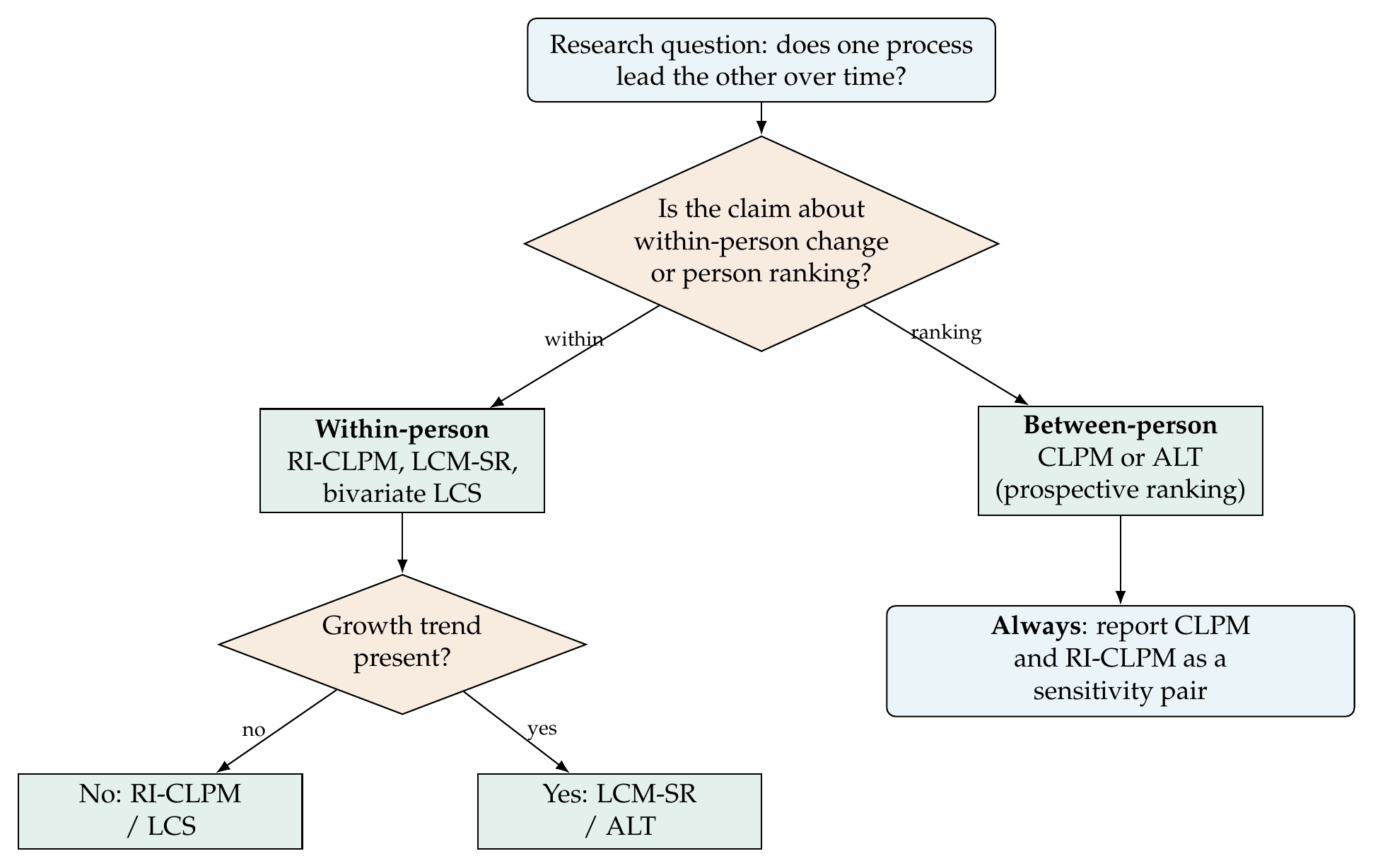
Note. The research question’s phrasing selects the estimand, and the estimand selects the family member. A within-person claim points to the RI-CLPM, LCM-SR, or bivariate LCS; a between-person prospective claim can be served by the CLPM or ALT. Whenever a directional claim is at stake, both the CLPM and the RI-CLPM are reported so the conclusion’s dependence on the modeling choice is visible.
21.4.2 The Measurement-Error Layer
A second refinement cuts across the whole family: the variables are measured with error, and unmodeled error damages the lagged structure asymmetrically. The reason is that measurement error attenuates the autoregression, since a fallible score predicts its own fallible future less well than a true score predicts its true future, and the attenuated autoregression leaves stability unexplained that the cross-lag then absorbs. Figure 21.6 demonstrates this on a two-process system with a true cross-lag of \(0.15\) and a null reverse path, fitting the observed-score CLPM at reliabilities from one down to one half. At perfect reliability the model recovers the truth. As reliability falls, the autoregression attenuates from \(0.50\) toward \(0.25\), the true cross-lag shrinks from \(0.15\) toward \(0.12\), and, most tellingly, the null cross-lag inflates away from zero toward \(0.03\): measurement error can manufacture the appearance of a reciprocal effect that is not there. The remedy is to model the error, either with multiple indicators and a latent-variable version of the panel model, which brings in the longitudinal invariance apparatus of Chapter 18, or, when only a single indicator is available, with a reliability correction that fixes the indicator’s error variance to a defensible value. The asymmetry of the damage, worst for the cross-lags, is a reason the latent-variable treatment matters most precisely for the reciprocal-effect questions this chapter is about.
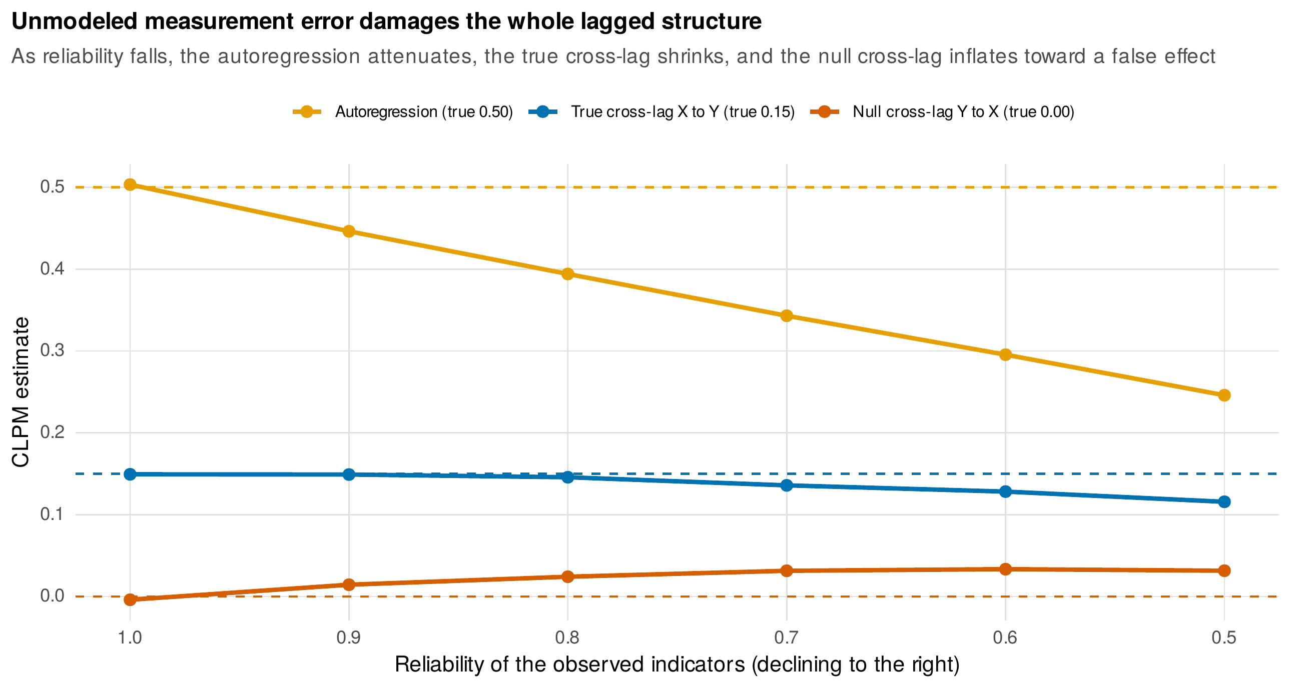
Note. Observed-score CLPM estimates from a two-process system as indicator reliability declines from one (left) to one half (right); dashed lines are the generating values, averaged over 60 replications per level. The autoregression attenuates, the true cross-lag shrinks, and the null cross-lag inflates toward a false positive. Modeling the error, through multiple indicators or a single-indicator reliability correction, is the remedy.
21.5 Causal Inference for Panel Data
Naming the estimand raises the question of what a panel design can license as a causal claim. The honest answer is modest, and it is best reasoned through directed acyclic graphs, the causal-inference tool introduced in Chapter 3 and applied here to the panel structure. Figure 21.7 draws two panel DAGs. The left panel shows time-varying confounding: an unobserved cause \(U_t\) that changes over time and affects both variables at each wave. The random intercept of the RI-CLPM removes a confounder only if it is time-invariant, a stable trait that is the same at every wave; a time-varying confounder like \(U_t\) passes straight through, because it is not constant and so is not absorbed by a constant latent factor. This is the sharp limit on the RI-CLPM’s much-advertised immunity to confounding, and it is why Table 21.3 lists time-varying confounding as a standing caution: the within-person cross-lag is unbiased for the causal effect only under the assumption, rarely testable, that all confounding is time-invariant.
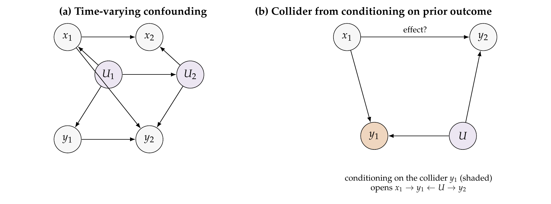
Note. (a) A time-varying confounder \(U_t\) (purple) affects both variables at every wave; because it is not constant, the random intercept of the RI-CLPM does not remove it, and the cross-lag \(x_1 \to y_2\) remains confounded. (b) Conditioning on the prior outcome \(y_1\) (shaded), which every cross-lagged model does, opens a non-causal path when \(y_1\) is a collider, a common effect of \(x_1\) and an unobserved cause \(U\) that also affects \(y_2\); the induced \(x_1\)-to-\(U\) association biases the estimated effect of \(x_1\) on \(y_2\). Person-level fixed effects remove time-invariant confounders only.
The right panel of Figure 21.7 shows a subtler hazard. Every cross-lagged model conditions on the prior outcome, regressing \(y_2\) on \(y_1\) to control for stability. If \(y_1\) shares an unobserved common cause with \(y_2\), then conditioning on \(y_1\), which is a collider on the path from \(x_1\) through that common cause to \(y_2\), can open a spurious association even when \(x_1\) has no effect on \(y_2\). Controlling for the prior outcome, the very move that defines the cross-lagged approach, is therefore not automatically benign; it can introduce bias rather than remove it. This is the deep reason the causal reading of any cross-lag rests on assumptions that the data cannot verify, and why the sensible-claims ladder of Table 21.4 keeps association, within-person prospective prediction, and causal effect on separate rungs, each rung requiring more than the last. The broader program of stating causal estimands and assumptions explicitly for longitudinal observational data, of which the panel case is one instance, is set out in the outcome-wide template of VanderWeele, Mathur, and Chen (2020).
Table 21.4. A ladder of defensible claims from panel data.
| Rung | Claim | What it requires |
|---|---|---|
| 1 | Association | Two variables covary across waves. Minimal; says nothing about direction or person versus occasion. |
| 2 | Prospective prediction (between) | One variable’s level forecasts the other’s later level in the ranking of persons. Requires temporal order; a CLPM or ALT estimand. |
| 3 | Within-person prospective prediction | A person’s deviation from their own norm forecasts their later deviation on the other variable. Requires the RI-CLPM or LCM-SR and stationarity. |
| 4 | Causal effect | The within-person effect equals what a manipulation would produce. Requires no unmeasured time-varying confounding, correct functional form, and no collider bias from conditioning on the prior outcome. Rarely licensed by observational panels. |
Note. Each rung demands strictly more than the one below. Panel data most defensibly support rungs one through three; rung four requires assumptions that observational designs cannot verify and that should be stated, probed, and reported as such.
21.5.1 The Econometric Bridge
Economists attack the same within-person estimand with a different tool, the fixed-effects estimator, which removes each person’s stable level by subtracting their own mean from every score before estimating the dynamics, the within transformation. Applied to a dynamic panel, regressing a variable on its own and the other’s person-mean-centered lag, this is the econometric sibling of the RI-CLPM’s within-person cross-lag, and it is instructive to run both on the same data. Figure 21.8 plots the four dynamic parameters from a hand-computed fixed-effects regression against the RI-CLPM estimates on panel_sim. The two cross-lags agree closely and lie on the diagonal: the fixed-effects estimator recovers the \(x \to y\) effect at \(0.199\), essentially identical to the RI-CLPM’s \(0.201\) and the truth of \(0.20\). The autoregressions, however, diverge sharply, with the fixed-effects estimates near \(0.05\) against the RI-CLPM’s \(0.41\). This is not a coding error but the Nickell bias: person-mean-centering a dynamic panel with few waves induces a correlation between the demeaned lagged predictor and the demeaned error, which biases the autoregression downward, severely so when the number of waves is small. The remedy in econometrics is either the maximum-likelihood structural formulation of Allison, Williams, and Moral-Benito (2017), which recovers the within-person effects without the small-sample bias and is close in spirit to the RI-CLPM, or the instrumental-variable generalized method of moments of Arellano and Bond (1991), which instruments the differenced lag with earlier levels. The convergence of two traditions, psychometric and econometric, on the same within-person estimand is a reassuring check, and their divergence on the autoregression is a reminder that small-wave dynamic panels are hard for every method.
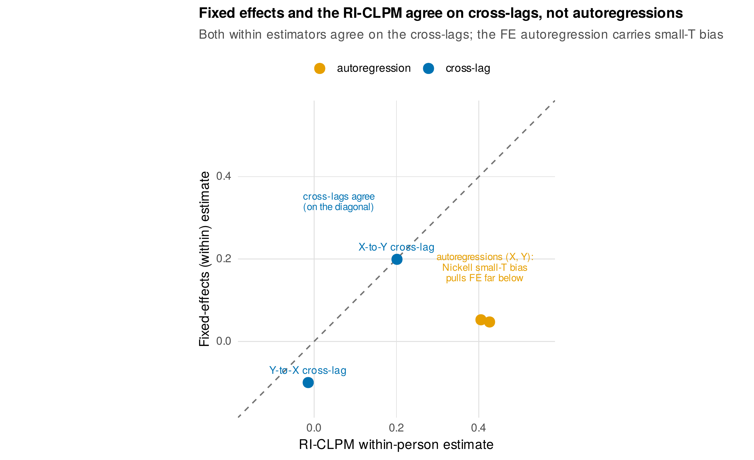
Note. Each point is one dynamic parameter, its RI-CLPM within-person estimate on the horizontal axis and its hand-computed fixed-effects estimate on the vertical axis; the dashed line is equality. The two cross-lags (blue) agree and lie on the diagonal. The two autoregressions (orange) fall far below it because the fixed-effects estimator carries Nickell bias when the number of waves is small; the maximum-likelihood formulation of Allison and colleagues corrects it.
An applied echo of the signature exhibit appears when the family is fitted to the school_panel data, an eight-hundred-student panel on engagement and achievement over four terms. The constrained CLPM reports a standardized engagement-to-achievement cross-lag of \(0.086\) and an achievement-to-engagement cross-lag of \(0.103\), both significant, the familiar picture of a reciprocal loop. The RI-CLPM, adding the random intercepts, finds a stable between-person correlation of \(0.53\) between the two traits and reduces both within-person cross-lags to \(0.05\), neither significant. The reciprocal loop the CLPM reported is, once the stable trait is separated out, largely a statement that students who are more engaged than others also achieve more than others, not that a student’s engaging more than usual raises their own later achievement. Whether the small within-person cross-lags are truly null or merely underpowered is itself worth stating, and it is the kind of nuance the sensitivity pair is meant to surface.
21.6 Longitudinal Mediation
Mediation, the claim that \(x\) affects \(y\) through an intermediary \(m\), is inherently about process over time, and analyzing it with variables measured at a single occasion imports a hidden and often severe bias. Maxwell and Cole (2007) proved the general result: when the true process is a longitudinal chain in which \(x\) affects later \(m\) which affects still later \(y\), a cross-sectional mediation analysis estimating all three variables at one wave recovers the true longitudinal indirect effect only under conditions so restrictive as to be implausible, and in general it can overstate, understate, or reverse the sign of the indirect effect. Figure 21.9 shows the divergence on a clean simulated chain whose true longitudinal indirect effect is \(0.160\): the correctly specified longitudinal model, in which each link respects the temporal lag and controls for the mediator’s and outcome’s own past, recovers \(0.159\), while the cross-sectional analysis of the same generating process returns \(0.087\), a little more than half the truth. The direction of the bias depends on the autoregressive parameters, which is exactly Maxwell and Cole’s point: the cross-sectional shortcut is not conservative, it is simply wrong by an amount and sign one cannot know without the longitudinal model.
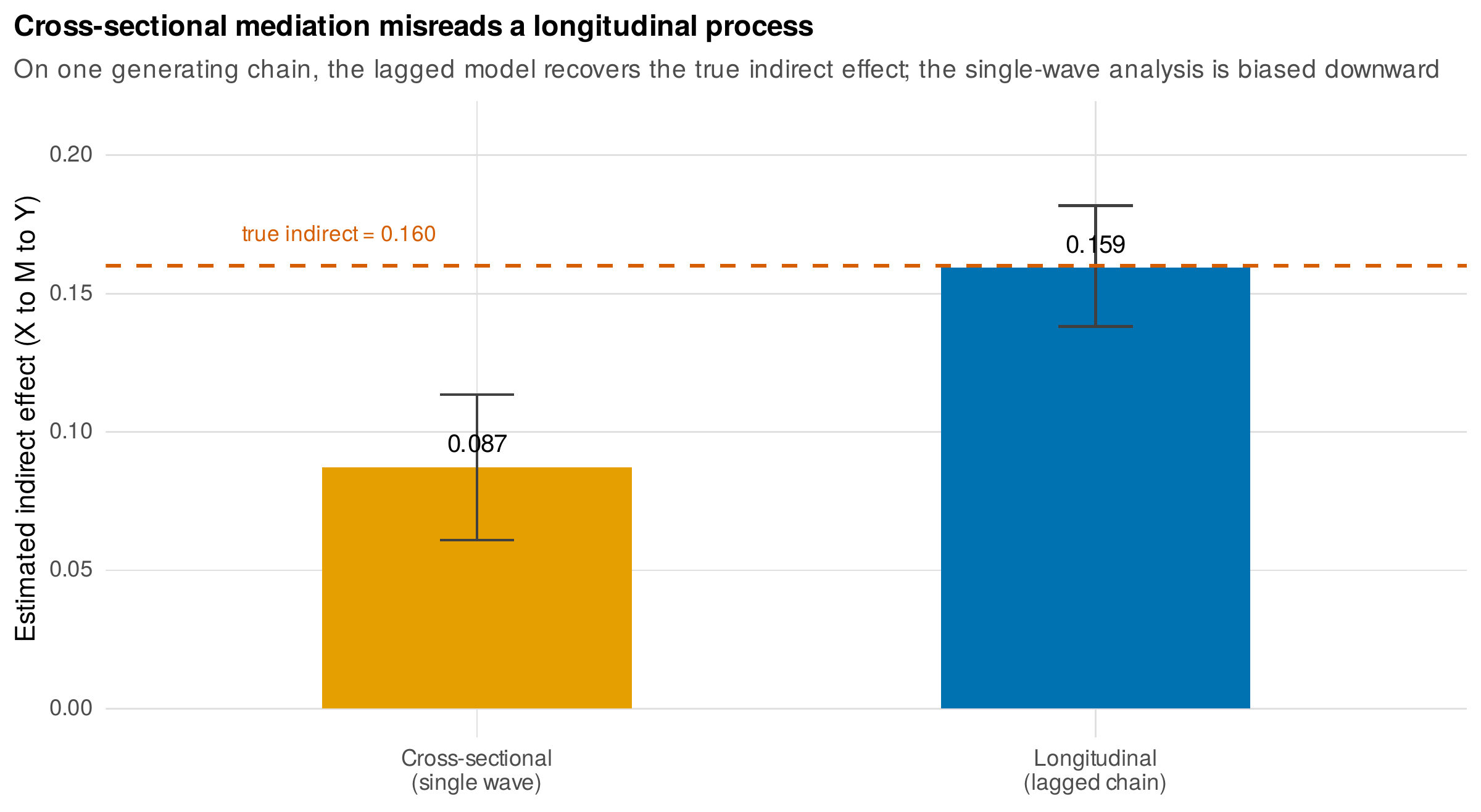
Note. Estimated indirect effect from a single-wave cross-sectional mediation and from a correctly lagged longitudinal mediation, both fitted to the same generating chain whose true longitudinal indirect effect is the dashed line; bars are means and whiskers the 2.5th-to-97.5th percentile spread across 80 simulated samples. The lagged model recovers the truth; the cross-sectional analysis is biased downward here, and in general its bias can run in either direction.
The correct designs are the half-longitudinal and full longitudinal mediation models in the tradition of Cole and Maxwell (2003), which respect temporal order by placing \(x\) before \(m\) before \(y\) and controlling each variable’s own prior level, and Selig and Preacher (2009) survey their variants for developmental data. The worked example ships as part of the analysis script: on the school_panel data, the indirect effect of engagement at the first term on achievement at the third, through study time at the second, is estimated at \(0.035\) with a Monte Carlo 95% confidence interval of \([0.021, 0.052]\), computed by drawing the two path coefficients from their joint sampling distribution and taking the percentiles of their product, the method of choice for indirect effects because the product of two normal coefficients is not itself normal and the naive symmetric interval misfires. That estimate is honestly a lower bound on the structural within-person indirect effect, which the generating process sets at \(0.105\), because the autoregressive mediation on raw scores does not partial out the stable traits and so attenuates the within-person paths, the same within-between lesson in mediational form. The frontier, an RI-CLPM-based mediation that estimates the indirect effect purely within persons, is an active and unsettled methodological area, and the honest report states the estimand, uses the Monte Carlo interval, and flags that the trait-adjusted within-person indirect effect requires the fuller model. A pitfall box collects the mediation and interpretation errors this chapter has warned against.
Common Pitfall • Four errors in reciprocal-effects and mediation practice
First, standardizing each wave separately and then comparing cross-lags across waves confounds changes in the coefficient with changes in the variables’ variances; standardize once, on a common metric, or compare unstandardized coefficients. Second, reading an RI-CLPM within-person cross-lag as the effect an intervention would produce overclaims: it is a short-run within-person association under stated assumptions, not a policy effect. Third, a two-wave design cannot separate a stable trait from within-person dynamics and cannot identify the RI-CLPM, so a two-wave cross-lagged analysis is a CLPM whatever it is called. Fourth, estimating mediation from three cross-sectional regressions, or from a single wave of a longitudinal process, imports the Maxwell-Cole bias and can report an indirect effect of the wrong size or sign.
21.7 Workflow and Reporting
The practical deliverable of this chapter is a workflow that turns a reciprocal-effects question into a defensible analysis, drawn in Figure 21.10. It begins not with a model but with the estimand: state whether the claim is about how persons rank or about how a person’s own deviations propagate. It proceeds to the measurement layer, deciding whether multiple indicators and a longitudinal invariance check are available or whether a single-indicator reliability correction must stand in, because measurement error damages cross-lags asymmetrically. It fits the candidate models the estimand implies, always including the CLPM and the RI-CLPM as a sensitivity pair when the claim is directional, and it compares them not only on fit but on whether the substantive conclusion is stable across them. It reports, finally, in the language the claims ladder licenses, no higher than the rung the design supports. Table 21.5 is the reporting checklist, and the software box points to the tools.
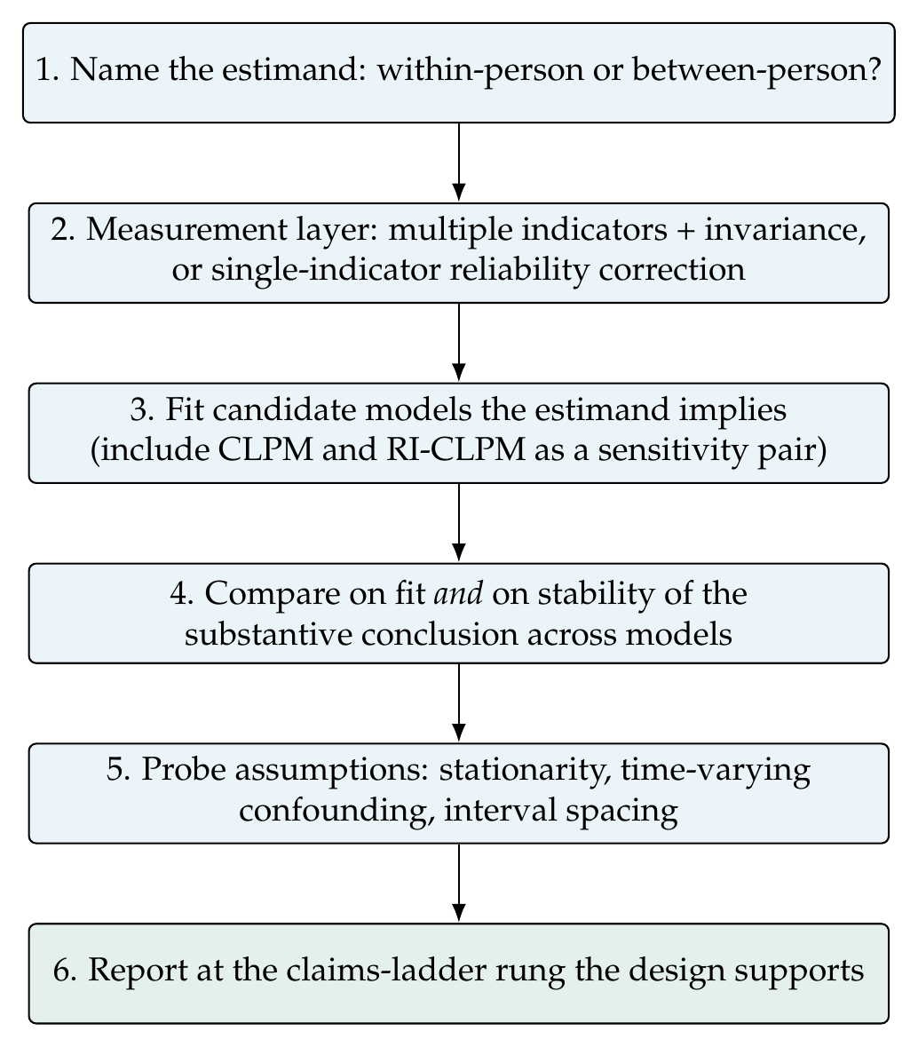
Note. The workflow places the estimand before the model, inserts the measurement layer before estimation, mandates the CLPM and RI-CLPM as a sensitivity pair for directional claims, and ties the language of the conclusion to the rung of the claims ladder (Table 21.4) that the design can support.
Table 21.5. Reporting checklist for reciprocal-effects studies.
| Item | |
|---|---|
| 1 | The estimand, stated as a within-person or between-person quantity, before any model |
| 2 | Number of waves, spacing, and whether spacing is equal; the stationarity assumption and its test |
| 3 | Measurement model: indicators per construct, invariance results, or the reliability correction used |
| 4 | The models fitted, with the CLPM and RI-CLPM both reported when the claim is directional |
| 5 | Standardized within-person cross-lags with confidence intervals, and the random-intercept variances and covariance |
| 6 | Fit indices for each model and whether the substantive conclusion is stable across them |
| 7 | Assumption probes: time-varying confounding considered, collider risk from conditioning on the prior outcome acknowledged |
| 8 | Conclusion phrased at the claims-ladder rung the design supports, no higher |
Note. The checklist operationalizes the estimand-first, sensitivity-reporting stance. A directional claim from panel data that omits the RI-CLPM contrast, or that phrases its conclusion above the supported rung, is incomplete.
Software Note • cross-lagged panel models across programs
In lavaan, the CLPM is an ordinary path model on the observed scores, and the RI-CLPM is built by adding the random-intercept factors with unit loadings, the within-person components with unit loadings, and the observed residual variances fixed to zero, exactly as in the shipped generator; the templates distributed by Mulder and Hamaker (2021) follow the same conventions. In Mplus the RI-CLPM is written with the random intercepts BY the observed scores at unit loadings and the within-person components defined likewise, with the dynamics on the within factors. The fixed-effects bridge is computed in R by person-mean-centering and regressing, as the analysis script does, or with the plm and fixest packages where available; for the maximum-likelihood dynamic panel that avoids Nickell bias, the approach of Allison and colleagues (2017) is implemented as a constrained structural equation model. The full workflow, both simulations, the family fits, the fixed-effects reconciliation, the reliability sweep, and the mediation, is the shipped ch21_analysis_V01.R, with figures in ch21_figures_V01.R and the datasets built by gen_panel_sim_V01.R and gen_school_panel_V01.R.
Chapter Summary
The cross-lagged panel model reads reciprocal influence from lagged regressions, but when stable between-person differences are present, and they nearly always are, its single autoregression cannot separate stable trait from dynamic carryover, and its cross-lags absorb the difference, inflating, attenuating, or inventing reciprocal effects, as the signature simulation shows by reporting a significant reverse effect whose true value is zero. The random intercept cross-lagged panel model adds a stable-trait factor per variable and moves the dynamics onto within-person components, recovering the within-person truth and reinterpreting every cross-lag as a within-person quantity, at the cost of requiring at least three waves and a stationarity assumption. The move from CLPM to RI-CLPM is a change of estimand, not a pure correction, and the counter-current, that within-person effects are short-run and occasion-specific and that between-person prospective questions are sometimes the right ones, deserves full weight; the book’s discipline is to name the estimand first and to report the CLPM and RI-CLPM as a sensitivity pair for any directional claim. The wider family, ALT, LCM-SR, GCLM, and the bivariate latent change score model, offers members matched to different assumptions about trait, growth, and dynamics. Causal claims from panel data are bounded: person-level fixed effects remove only time-invariant confounding, conditioning on the prior outcome can open collider bias, and the fixed-effects and RI-CLPM within-person estimators agree on cross-lags while diverging on autoregressions through Nickell bias. Longitudinal mediation must respect temporal order, since cross-sectional mediation of a longitudinal process is biased by an unknown amount and sign, and indirect effects are reported with Monte Carlo confidence intervals. The claims ladder keeps association, within-person prediction, and causal effect on separate rungs, and the conclusion is phrased no higher than the design supports.
Exercises
- 21.1 Reproduce the signature exhibit. Fit the CLPM and RI-CLPM to
panel_sim, confirm the spurious cross-lag and the recovered truth, then raise and lower the trait correlation in the generating script and chart how the CLPM’s bias in the cross-lags tracks the share of variance that is stable trait. - 21.2 Fit the family. On the
school_panelengagement and achievement data, fit the CLPM, RI-CLPM, ALT, LCM-SR, and bivariate latent change score model; assemble a comparison in the style of Table 21.2, and write the estimand-based adjudication of which model answers which question. - 21.3 DAG exercise. Draw the assumptions, as a directed acyclic graph, under which the CLPM cross-lag equals a causal effect, then identify a plausible time-varying confounder for an engagement-achievement study and show where the RI-CLPM’s immunity fails.
- 21.4 Fixed-effects reconciliation. Compute the within (fixed-effects) estimator on
panel_simby person-mean-centering, compare it to the RI-CLPM, and explain the divergence on the autoregressions in terms of Nickell bias and the number of waves. - 21.5 Longitudinal mediation. Fit the longitudinal mediation on
school_panelwith a Monte Carlo confidence interval, then fit the cross-sectional mediation on a single wave, and explain the divergence in terms of the Maxwell-Cole result. - 21.6 Peer-review drill. Given a manuscript excerpt that reports a CLPM cross-lag as a causal effect, write a referee report that names the estimand problem, requests the RI-CLPM sensitivity analysis, and specifies the claims-ladder rung the design can support.
References
Allison, P. D. (2009). Fixed effects regression models. SAGE Publications. https://doi.org/10.4135/9781412993869
Allison, P. D., Williams, R., & Moral-Benito, E. (2017). Maximum likelihood for cross-lagged panel models with fixed effects. Socius: Sociological Research for a Dynamic World, 3, Article 2378023117710578. https://doi.org/10.1177/2378023117710578
Arellano, M., & Bond, S. (1991). Some tests of specification for panel data: Monte Carlo evidence and an application to employment equations. The Review of Economic Studies, 58(2), 277–297. https://doi.org/10.2307/2297968
Berry, D., & Willoughby, M. T. (2017). On the practical interpretability of cross-lagged panel models: Rethinking a developmental workhorse. Child Development, 88(4), 1186–1206. https://doi.org/10.1111/cdev.12660
Bollen, K. A., & Curran, P. J. (2004). Autoregressive latent trajectory (ALT) models: A synthesis of two traditions. Sociological Methods & Research, 32(3), 336–383. https://doi.org/10.1177/0049124103260222
Cole, D. A., & Maxwell, S. E. (2003). Testing mediational models with longitudinal data: Questions and tips in the use of structural equation modeling. Journal of Abnormal Psychology, 112(4), 558–577. https://doi.org/10.1037/0021-843X.112.4.558
Curran, P. J., Howard, A. L., Bainter, S. A., Lane, S. T., & McGinley, J. S. (2014). The separation of between-person and within-person components of individual change over time: A latent curve model with structured residuals. Journal of Consulting and Clinical Psychology, 82(5), 879–894. https://doi.org/10.1037/a0035297
Hamaker, E. L. (2026). The within-between dispute in cross-lagged panel research and how to move forward. Psychological Methods, 31(1), 56–76. https://doi.org/10.1037/met0000600
Hamaker, E. L., Kuiper, R. M., & Grasman, R. P. P. P. (2015). A critique of the cross-lagged panel model. Psychological Methods, 20(1), 102–116. https://doi.org/10.1037/a0038889
Hamaker, E. L., & Muthén, B. (2020). The fixed versus random effects debate and how it relates to centering in multilevel modeling. Psychological Methods, 25(3), 365–379. https://doi.org/10.1037/met0000239
Lucas, R. E. (2023). Why the cross-lagged panel model is almost never the right choice. Advances in Methods and Practices in Psychological Science, 6(1), Article 25152459231158378. https://doi.org/10.1177/25152459231158378
Lüdtke, O., & Robitzsch, A. (2022). A comparison of different approaches for estimating cross-lagged effects from a causal inference perspective. Structural Equation Modeling: A Multidisciplinary Journal, 29(6), 888–907. https://doi.org/10.1080/10705511.2022.2065278
Maxwell, S. E., & Cole, D. A. (2007). Bias in cross-sectional analyses of longitudinal mediation. Psychological Methods, 12(1), 23–44. https://doi.org/10.1037/1082-989X.12.1.23
Mulder, J. D., & Hamaker, E. L. (2021). Three extensions of the random intercept cross-lagged panel model. Structural Equation Modeling: A Multidisciplinary Journal, 28(4), 638–648. https://doi.org/10.1080/10705511.2020.1784738
Orth, U., Clark, D. A., Donnellan, M. B., & Robins, R. W. (2021). Testing prospective effects in longitudinal research: Comparing seven competing cross-lagged models. Journal of Personality and Social Psychology, 120(4), 1013–1034. https://doi.org/10.1037/pspp0000358
Rogosa, D. (1980). A critique of cross-lagged correlation. Psychological Bulletin, 88(2), 245–258. https://doi.org/10.1037/0033-2909.88.2.245
Rohrer, J. M., & Murayama, K. (2023). These are not the effects you are looking for: Causality and the within-/between-persons distinction in longitudinal data analysis. Advances in Methods and Practices in Psychological Science, 6(1), Article 25152459221140842. https://doi.org/10.1177/25152459221140842
Selig, J. P., & Preacher, K. J. (2009). Mediation models for longitudinal data in developmental research. Research in Human Development, 6(2–3), 144–164. https://doi.org/10.1080/15427600902911247
Usami, S. (2021). On the differences between general cross-lagged panel model and random-intercept cross-lagged panel model: Interpretation of cross-lagged parameters and model choice. Structural Equation Modeling: A Multidisciplinary Journal, 28(3), 331–344. https://doi.org/10.1080/10705511.2020.1821690
Usami, S., Murayama, K., & Hamaker, E. L. (2019). A unified framework of longitudinal models to examine reciprocal relations. Psychological Methods, 24(5), 637–657. https://doi.org/10.1037/met0000210
VanderWeele, T. J., Mathur, M. B., & Chen, Y. (2020). Outcome-wide longitudinal designs for causal inference: A new template for empirical studies. Statistical Science, 35(3), 437–466. https://doi.org/10.1214/19-STS728
Zyphur, M. J., Allison, P. D., Tay, L., Voelkle, M. C., Preacher, K. J., Zhang, Z., Hamaker, E. L., Shamsollahi, A., Pierides, D. C., Koval, P., & Diener, E. (2020a). From data to causes I: Building a general cross-lagged panel model (GCLM). Organizational Research Methods, 23(4), 651–687. https://doi.org/10.1177/1094428119847278
Zyphur, M. J., Voelkle, M. C., Tay, L., Allison, P. D., Preacher, K. J., Zhang, Z., Hamaker, E. L., Shamsollahi, A., Pierides, D. C., Koval, P., & Diener, E. (2020b). From data to causes II: Comparing approaches to panel data analysis. Organizational Research Methods, 23(4), 688–716. https://doi.org/10.1177/1094428119847280