Chapter 22
Growth Mixture, Latent Class Growth, and Latent Transition Models
Every model so far in Part V has assumed that one set of parameters describes everyone: a single growth curve with individual variation around it, a single set of cross-lagged dynamics. This chapter entertains a different possibility, that the population is a mixture of qualitatively distinct subgroups, each with its own trajectory or its own sequence of states. The idea is intuitive and, in fields from developmental psychopathology to substance-use research, enormously popular: rather than a continuum of change, perhaps there are types, early responders and non-responders, resilient and susceptible, persistent and desisting. The tools that formalize this intuition, latent class growth analysis, growth mixture modeling, and latent transition analysis, are among the most powerful and the most abused in the longitudinal toolkit. They will happily return classes from data that contain none, and a decade of methodological work has shown that a single skewed population is enough to fool them. The chapter therefore carries a dual mandate that its predecessors did not: it must teach the machinery well enough to use it competently, and it must install, as a permanent reflex, the skepticism that keeps the machinery from manufacturing subgroups that are statistical artifacts rather than real kinds. Competence and doubt are developed together, because in mixture modeling they are the same skill.
Learning Objectives
After working through this chapter, you should be able to: (1) distinguish latent class growth analysis, which fixes within-class variance to zero, from growth mixture modeling, which frees it, and predict how the choice changes the number and meaning of classes; (2) execute a multi-criteria class-enumeration protocol using information criteria, the bootstrap likelihood ratio test, entropy, class sizes, interpretability, and replication, never a single index; (3) diagnose overextraction, above all the Bauer-Curran result that nonnormal single populations yield spurious classes, and run the anti-fragility checks; (4) relate classes to covariates and distal outcomes with three-step methods and explain why classify-then-regress and one-step approaches both fail; (5) specify a latent transition model with invariant status measurement and interpret its transition matrix; (6) connect latent transition analysis to the hidden Markov tradition; and (7) report a mixture analysis to the emerging GRoLTS standard.
22.1 Heterogeneity: Dimensional or Categorical?
Before any software runs, a substantive question must be faced: is the heterogeneity in a set of trajectories a matter of degree or of kind? A dimensional view holds that people differ continuously, some declining faster than others around a common process, and that any grouping is a convenient summary of a continuum. A categorical view holds that the population contains genuinely distinct subtypes, each governed by its own process, so that a person belongs to one type and the types are real. The distinction matters because the two views license different claims. A dimensional finding supports statements about predictors of the rate of change; a categorical finding, if true, supports statements about kinds of people, about who belongs to the persistent versus the desisting type, and invites categorical interventions. Mixture models fit the categorical view, and their seductiveness is precisely that they return categories whether or not the categories are real.
The cautionary exemplar is Moffitt’s (1993) developmental taxonomy of antisocial behavior, which proposed two qualitatively distinct types of offenders, a small life-course-persistent group and a larger adolescence-limited group, each with a different etiology. The taxonomy was enormously influential and organized decades of research, and it is genuinely theory-driven rather than an artifact of a fitting algorithm. But it also became the template for a style of empirical work in which a growth mixture model is fitted, a handful of classes emerge, and the classes are promptly reified as discovered types with names and clinical significance, often on the strength of a single information criterion. The distance between Moffitt’s theory-first taxonomy and the software-first extraction of trajectory classes is the distance this chapter asks readers to keep in view. Classes can be a real feature of the world, a useful approximation to a continuum, or a mirage; the model cannot tell these apart, and only substantive theory, replication, and the diagnostics developed below can (Bauer, 2007).
Figure 22.1 makes the epistemic point concrete. It shows three sets of trajectories that look much alike, spaghetti plots of the kind that open countless mixture papers. The first is a single heterogeneous population, one process with wide individual variation. The second is a set of three latent class growth classes, crisp subgroups with no within-class variation beyond measurement noise. The third is three growth mixture classes, subgroups with their own internal spread. To the eye the three are nearly indistinguishable, and no amount of staring at raw trajectories will reveal which generative story produced them. That is the problem the rest of the chapter addresses, and the reason it insists that the answer cannot come from the data alone.
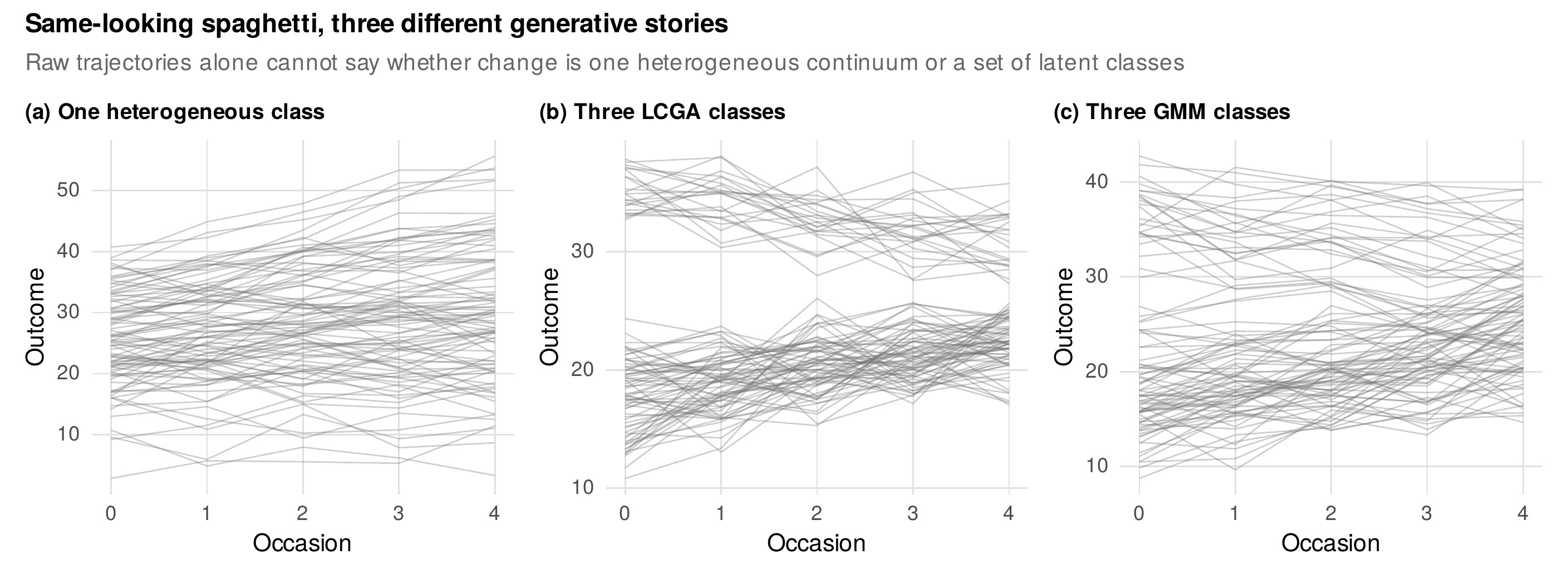
Note. The same style of spaghetti plot can arise from one heterogeneous population (a), from crisp latent class growth classes with no within-class variance (b), or from growth mixture classes with within-class spread (c). Raw trajectories cannot distinguish these accounts, which is why class enumeration and the diagnostics of this chapter, not visual inspection, must carry the argument.
The family of models that formalizes categorical heterogeneity descends from the single-class latent growth model of Chapter 19 by two elaborations. Freeing the growth means to differ across a set of latent classes, while forcing every person within a class onto the same curve except for measurement error, gives the latent class growth analysis (LCGA) model of the Nagin (1999) tradition. Additionally freeing the growth factors to vary within each class, so that each class is itself a small latent growth model, gives the growth mixture model (GMM) of the Muthén and Shedden (1999) tradition. The single-class growth model is the special case of either with one class. Accessible primers on the distinction are given by Jung and Wickrama (2008) and Ram and Grimm (2009), and comprehensive treatments by Masyn (2013) and Grimm, Ram, and Estabrook (2017). Table 22.1 lays out the three side by side, because the differences in what they assume produce large differences in what they conclude, most visibly in how many classes they extract.
Table 22.1. Latent growth, latent class growth, and growth mixture models compared.
| Feature | Latent growth (Ch. 19) | LCGA (Nagin) | GMM (Muthén) |
|---|---|---|---|
| Number of classes | One | Several | Several |
| Within-class growth variance | Freely estimated | Fixed to zero | Freely estimated |
| Class captures | Nothing (one population) | A distinct mean trajectory | A distinct trajectory with spread |
| Typical class count | — | More (absorbs variance as classes) | Fewer |
| Main risk | Misses subgroups if real | Overextraction from restrictiveness | Nonconvergence; overextraction from nonnormality |
| Reads heterogeneity as | Continuous | Categorical, crisp | Categorical, fuzzy |
Note. LCGA and GMM answer the categorical question differently. Because LCGA forbids within-class variation, it tends to need more classes to fit the same data, so LCGA and GMM class counts are not comparable, a point the pitfalls box returns to.
22.2 Specification and Estimation
The two models differ in one covariance restriction with large consequences. Write the growth model within class \(k\) as \(\mathbf{y}_i = \mathbf{Z}\bm{\beta}_k + \mathbf{Z}\mathbf{b}_i + \bm{\varepsilon}_i\), where \(\mathbf{Z}\) holds the time codes, \(\bm{\beta}_k\) is the class growth mean, \(\mathbf{b}_i\) are the person’s random deviations, and \(\bm{\varepsilon}_i\) is residual noise. LCGA sets the random-effect covariance to zero, \(\mathrm{Var}(\mathbf{b}_i)=\mathbf{0}\), so every member of a class shares the class curve exactly up to residual error; the classes are crisp lines and all within-class spread is noise. GMM frees that covariance, so each class is a cloud around its mean curve. Figure 22.2 draws the difference in the space of growth factors: LCGA sees a class as a point, GMM sees it as an ellipse. The restriction is consequential because a real population almost always has within-group variation, and a model that forbids it must represent that variation some other way, by adding classes. This is the mechanism behind LCGA’s tendency to extract more classes than GMM on the same data, and the reason their class counts must never be compared as if they meant the same thing.
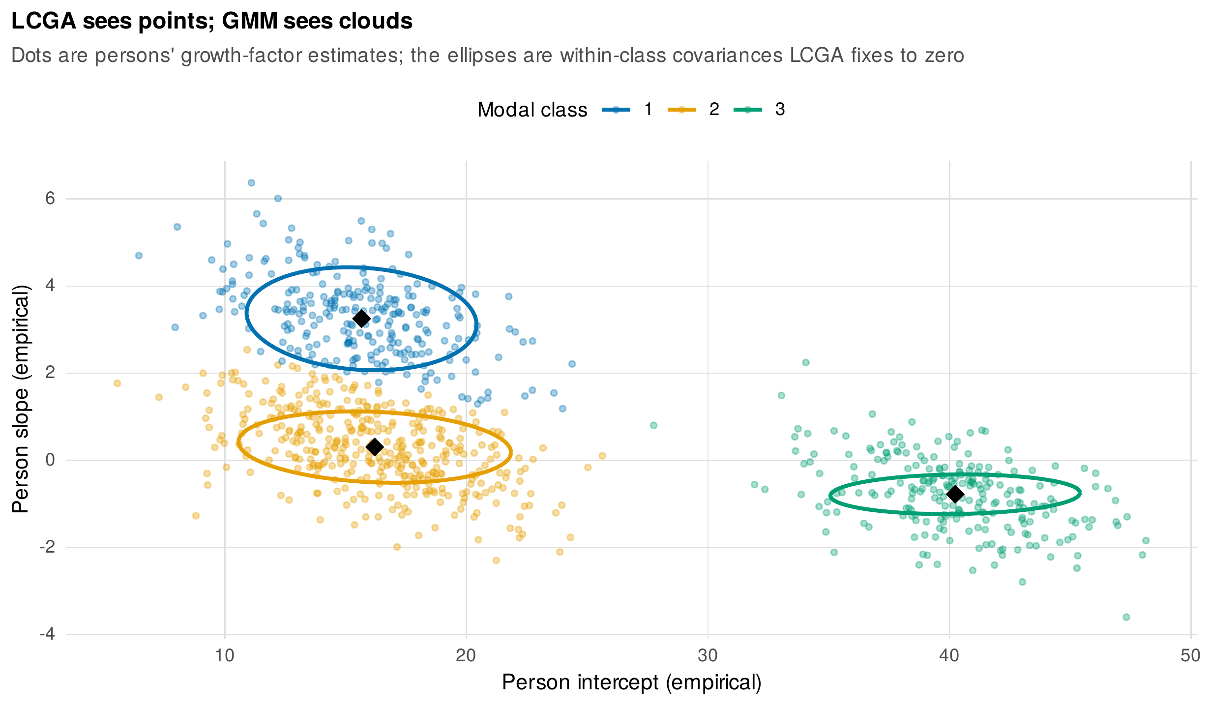
Note. Each dot is a person’s estimated growth factors from classes_sim; color is the modal growth mixture class. The ellipses are the growth mixture within-class covariances, the spread that LCGA fixes to zero, collapsing each class to the black point at its center. A population with genuine within-class variation forces LCGA to represent that variation by adding classes.
Within a chosen number of classes, both models are estimated by maximum likelihood through the expectation-maximization algorithm, which alternates between computing each person’s posterior probability of belonging to each class, given current parameters, and updating the parameters as posterior-probability-weighted quantities. The mixture likelihood sums over the unknown class memberships, and its surface is riddled with local maxima, so a single run from a single starting point is untrustworthy. The discipline the field has settled on is many random starts, dozens to hundreds, retaining the solution with the best log-likelihood and, crucially, confirming that this best value is replicated by several starts rather than reached once and never again; a best log-likelihood that appears only once is a red flag for a spurious solution. The foundations box states the likelihood and the algorithm; the practice box gathers the starts-and-seeds hygiene that reproducibility demands.
Foundations Box • The mixture likelihood, EM, and why entropy is not a fit index
For a \(K\)-class mixture the marginal density of person \(i\)’s data is \(f(\mathbf{y}_i)=\sum_{k=1}^{K}\pi_k\, f_k(\mathbf{y}_i\mid\bm{\theta}_k)\), a weighted sum of the within-class densities with mixing weights \(\pi_k\) summing to one. The log-likelihood \(\sum_i \log f(\mathbf{y}_i)\) cannot be maximized in closed form because the class labels are missing, so EM introduces the posterior probabilities \(\hat p_{ik}=\pi_k f_k(\mathbf{y}_i)/\sum_j \pi_j f_j(\mathbf{y}_i)\) in the expectation step and maximizes the expected complete-data log-likelihood, updating \(\pi_k\) as the mean posterior and \(\bm{\theta}_k\) as the posterior-weighted estimates, in the maximization step. Iterating increases the observed-data log-likelihood monotonically to a local maximum. Entropy, often reported alongside, is \(E_K = 1 - \sum_i\sum_k(-\hat p_{ik}\ln \hat p_{ik})/(N\ln K)\), and it measures how cleanly persons are classified, approaching one when posteriors are near zero or one. It says nothing about whether \(K\) is correct: a two-class model can classify crisply into two wrong classes. Entropy is a property of classification quality, to be reported for interpretability, never a criterion for choosing the number of classes.
In Practice • Random starts, seeds, and documenting the solution path
Treat the number of random starts as a reported analytic decision, not a default. For simple models dozens of starts may suffice; for GMM with freed within-class covariances, use many more and increase them until the best log-likelihood replicates across several independent starts. Set and report a seed so the solution is reproducible, and document the full path: the number of starts, how many converged, whether the best value replicated, and any boundary or nonconvergence problems encountered at each \(K\). Boundary solutions, negative variances, and nonconvergence are diagnostic information about model-data mismatch, not nuisances to be silently discarded. The analyses in this chapter were fitted with expectation-maximization written from scratch, seeded and multi-start, so that every step is inspectable; production work would use a dedicated package (the software box lists them), but the estimation realities, local maxima and the multiple-starts requirement above all, are identical.
22.3 Enumeration: The Multi-Criteria Protocol
Choosing the number of classes is the decision on which everything else rests, and it is genuinely hard because no single statistic settles it. The workhorse indices are the information criteria, which trade fit against complexity: the Bayesian information criterion (BIC), its sample-size-adjusted variant (aBIC), and the consistent AIC (CAIC), all smaller-is-better. In the Nylund, Asparouhov, and Muthén (2007) simulations, which remain the reference, the BIC and aBIC performed well while the ordinary AIC overextracted, and the bootstrap likelihood ratio test (BLRT), which compares a \(K\)-class model against a \(K-1\)-class model by simulating the null distribution of the likelihood ratio, was the most reliable single indicator. Alongside these sit entropy, reported for classification quality rather than selection; the size of the smallest class, since a class comprising two percent of the sample is rarely a defensible kind; substantive interpretability; and replication across split halves or independent samples. The protocol is to consult all of them, as a panel of evidence, never to read a single index as a verdict (Nylund-Gibson & Choi, 2018).
Figure 22.3 shows the panel assembled for the three-class classes_sim data. The information criteria elbow sharply and reach their minimum at three classes, with the BIC rising again at four. The bootstrap likelihood ratio test is significant when moving from one to two and from two to three classes, then not significant from three to four, the pattern that says a fourth class adds nothing. Entropy is high and the smallest class stays comfortably large through three classes, then the smallest class collapses as spurious fourth and fifth classes carve off slivers of the sample. Every criterion, read together, points to three, which is the truth. Table 22.2 catalogs the indices, their known behavior, and their proper role, and Table 22.3 states the book’s stepwise enumeration protocol in a form that can be preregistered.
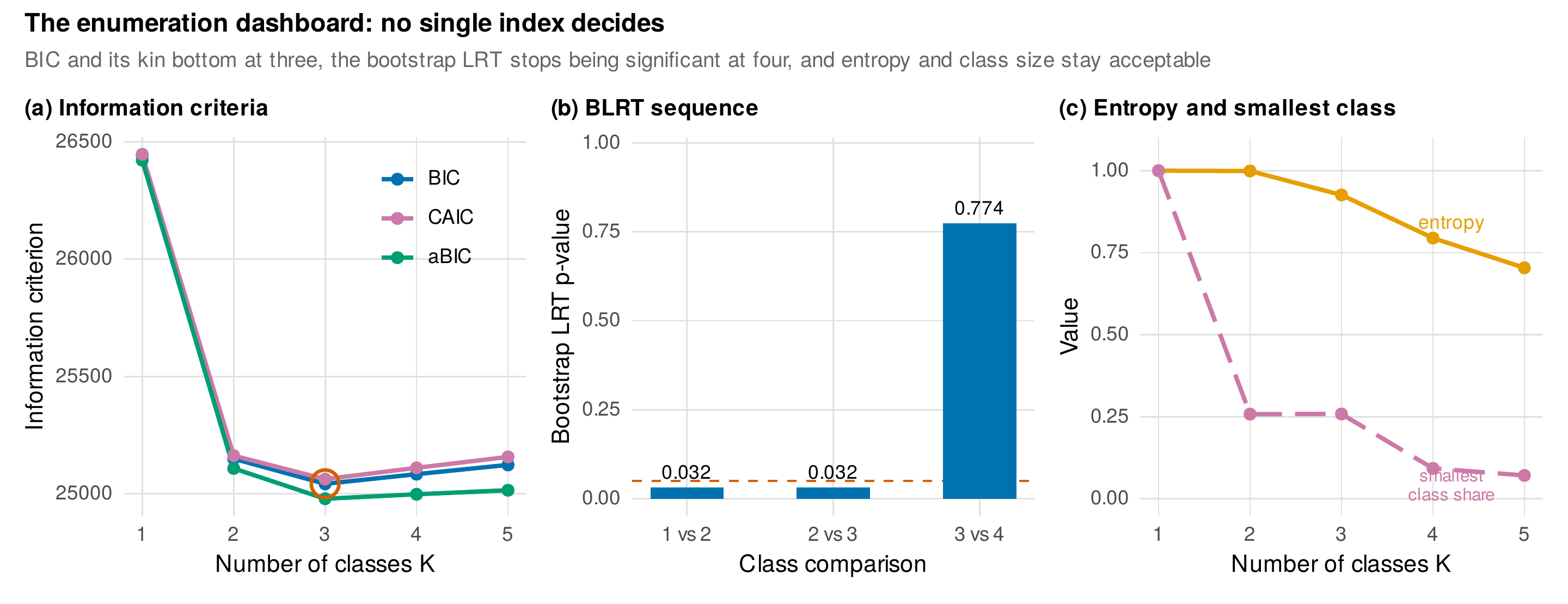
Note. Information criteria (a) elbow to their minimum at three classes; the bootstrap likelihood ratio test (b) is significant up to three classes and not significant for a fourth; entropy and the smallest-class share (c) remain acceptable through three, then the smallest class collapses as spurious classes appear. No single panel decides; their agreement does.
Table 22.2. Class-enumeration indices and their roles.
| Index | Behavior | Role in the protocol |
|---|---|---|
| BIC | Penalizes complexity heavily; reliable, mildly conservative | Primary index; look for the minimum or elbow |
| aBIC | Lighter sample-size adjustment; slightly less conservative | Corroborates BIC; useful at small \(N\) |
| CAIC | Consistent AIC; conservative like BIC | Corroborating information criterion |
| AIC | Overextracts in simulations | Not recommended for selection |
| BLRT | Bootstrapped null of the likelihood ratio; powerful | Test each \(K\) against \(K-1\); stop when nonsignificant |
| Entropy | Classification quality, not fit | Report for interpretability; never for selection |
| Smallest class | Size or proportion of the rarest class | Sanity screen; distrust slivers |
| Interpretability, replication | Substantive meaning; stability across samples | Co-equal criteria, not afterthoughts |
Note. The bootstrap likelihood ratio test and the BIC are the most trustworthy single indicators in the simulation literature, but the decision is multi-criteria: information criteria, the BLRT, class size, interpretability, and replication together.
22.3.1 The Bauer-Curran Warning
The single most important result in this literature is a negative one. Bauer and Curran (2003, 2004) showed that a growth mixture model fitted to data from a single population will extract multiple classes whenever that population is nonnormal, because a mixture of normals can approximate a skewed or heavy-tailed distribution, and the fitting algorithm will use extra classes to do exactly that. The classes in such a case are not subgroups; they are basis functions approximating a shape. The result is not a curiosity at the margin but a standing threat to every mixture analysis, because real psychological variables are routinely skewed. Figure 22.4 is the chapter’s signature exhibit. The data are a single skewed population, one group, generated with right-skewed intercepts and a common slope. Fitted with a normal growth mixture, the information criteria prefer several classes, and the model cheerfully partitions the skewed continuum into a low class and a high class divided at an arbitrary point in the tail. There are no subgroups; there is one skewed group, and the classes are an artifact of forcing normal components onto a nonnormal shape.
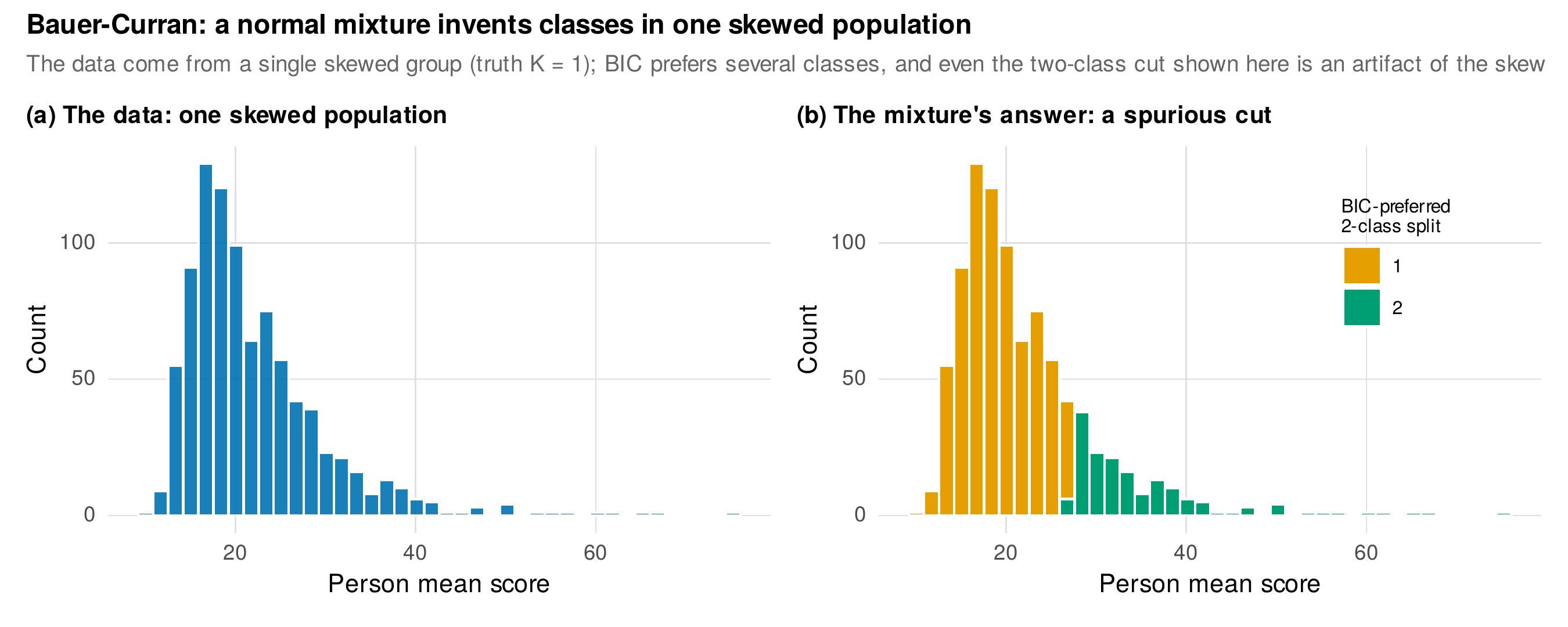
Note. Left: the data are one right-skewed population (true number of classes is one). Right: a normal growth mixture, preferred by the BIC over a single class, slices the continuum into spurious classes divided at an arbitrary point in the tail. The classes approximate the skew; they are not subgroups. Skew alone manufactures classes.
The defenses against this failure are specific and should be routine. The first is to ask whether the classes might be an artifact of distributional shape, which means fitting models that allow nonnormal within-class distributions, skew-normal or skew-\(t\) mixtures where the software supports them, and checking whether the extra classes survive when the components are allowed to be skewed. The second is a covariate-inclusion stability check: a class solution that changes substantially when a covariate is added, or that only appears in the covariate-free model, is suspect, because real subgroups should not dissolve when a predictor is introduced. The third is the comparison discipline of asking whether a continuous model, a single-class growth model with a nonnormal distribution or a factor model, fits the data as well as the mixture; if it does, parsimony and the Bauer-Curran result together counsel against reifying the classes. None of these is a guarantee, and the honest conclusion of the Bauer-Curran literature is epistemic humility: a well-fitting mixture is consistent with latent classes but does not establish them, and the language of a report should say so.
Table 22.3. The book’s class-enumeration protocol.
| Step | Action |
|---|---|
| 1 | Fit \(K=1\) through a generous maximum with a documented number of random starts; confirm the best log-likelihood replicates at each \(K\) |
| 2 | Assemble the information criteria (BIC, aBIC, CAIC) and read the minimum or elbow, not a single index |
| 3 | Run the bootstrap likelihood ratio test for successive \(K\); stop where it becomes nonsignificant |
| 4 | Screen entropy (for interpretability) and the smallest-class size (distrust slivers) |
| 5 | Probe the Bauer-Curran risk: nonnormal-component models, covariate-inclusion stability, and a continuous-model comparison |
| 6 | Check replication across split halves or independent cohorts |
| 7 | Adjudicate on substantive interpretability, preregistering the criteria where possible; report the full solution path |
Note. The protocol is deliberately multi-step and preregisterable. Its purpose is to make the number-of-classes decision a documented argument rather than the reading of one statistic.
The stability check of step six deserves its own illustration because it is the most neglected. Figure 22.5 refits the enumeration on two independent halves of the data. The three-class solution replicates: the BIC bottoms at three in both halves. A solution that appeared in the full sample but not in either half, or that gave three classes in one half and four in the other, would be a warning that the classes are unstable and probably not real. Replication is not a formality appended after selection; it is part of selection.
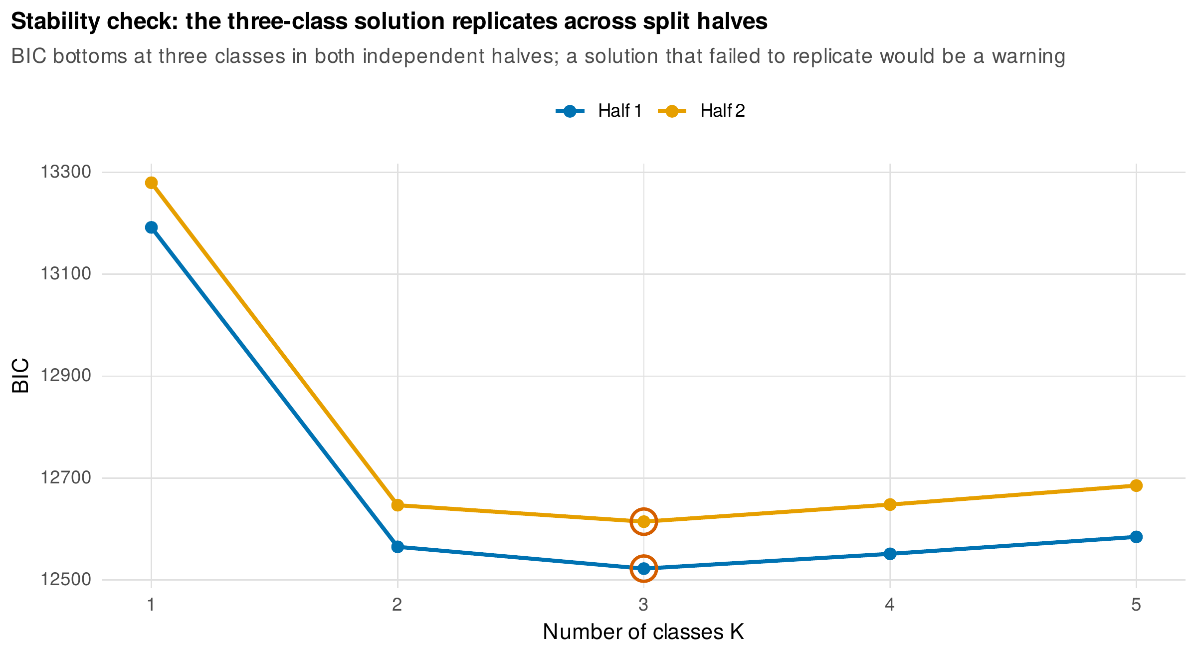
Note. The BIC bottoms at three classes in both independent halves of classes_sim, so the three-class solution replicates. A solution that failed to reappear in a held-out half, or that gave a different number of classes across halves, would be evidence of instability and grounds for doubt.
22.4 Classes in Context: Auxiliary Variables
A class solution is rarely the end of an analysis; the classes are meant to relate to something, to a predictor of membership or to a distal outcome. The naive way to do this, and the wrong way, is to assign each person to their most likely class and then treat that assignment as an observed variable in a regression, predicting the modal class from a covariate or predicting an outcome from the modal class. The problem is classification error. Modal assignment discards the posterior uncertainty, treating a person classified with probability \(0.6\) identically to one classified with probability \(0.99\), and the resulting misclassification attenuates every relationship the classes enter, biasing covariate effects and distal-outcome differences toward zero. The alternative of building the covariate into the mixture model itself, the one-step approach, avoids the attenuation but creates a different problem: the covariate then helps define the classes, so adding or removing a predictor reshapes the latent classes, and the measurement model is no longer separable from the structural question. Figure 22.6 diagrams why both naive routes fail and what the three-step logic does instead.
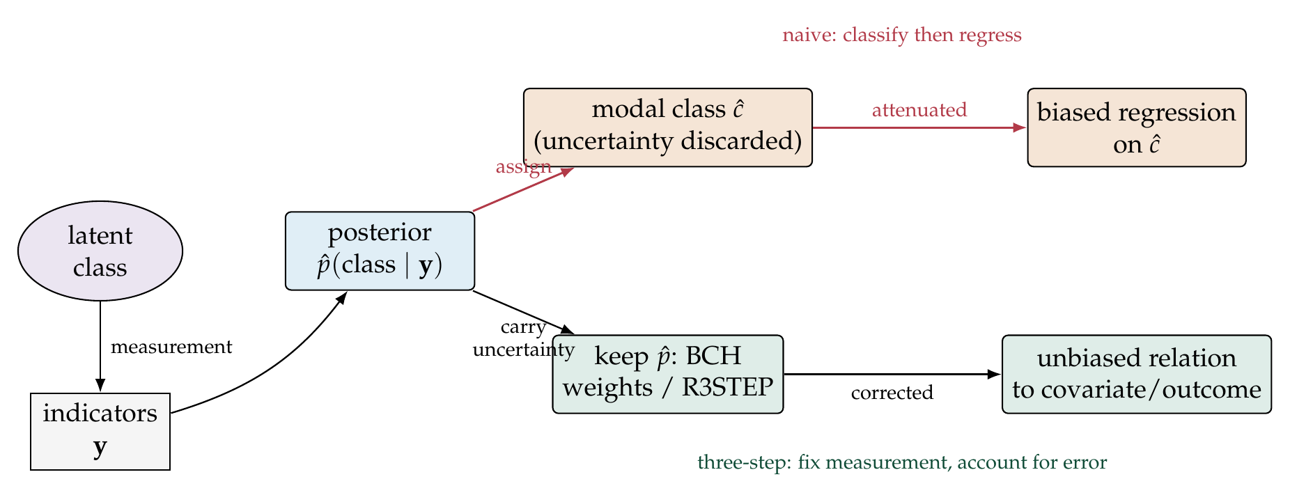
Note. The mixture yields posterior class probabilities. The naive route (top, red) collapses them to a modal class, discarding the classification uncertainty, so any regression on the modal class is attenuated by misclassification. The three-step route (bottom) fixes the measurement model, then carries the classification uncertainty into the analysis of covariates (R3STEP) or distal outcomes (BCH), correcting the error. The one-step alternative, not shown, lets the covariate reshape the classes.
The three-step approach separates the two concerns. It fixes the measurement model first, estimating the classes from the indicators alone; then it relates the classes to covariates and outcomes in a way that accounts for classification error rather than ignoring it. For a covariate predicting class membership the modern tool is the R3STEP method; for a distal outcome the tool is the BCH method of Vermunt (2010) and Bakk and Vermunt (2016), which descends from the Bolck, Croon, and Hagenaars (2004) insight that the classification error matrix can be estimated and inverted to undo the attenuation. The Mplus implementations of these steps are documented by Asparouhov and Muthén (2014), and Nylund-Gibson, Grimm, and Masyn (2019) compare the distal-outcome approaches directly. Table 22.4 maps the methods to the questions they answer. Figure 22.7 demonstrates the correction on the resp_classes data, a treatment-response mixture with three planted classes, early responders, gradual responders, and non-responders, whose membership is driven by baseline symptom severity and whose relapse risk differs by class. The recovered classes match the generating trajectories, with slopes near the true values of \(-3.0\), \(-1.5\), and \(-0.2\). On the distal outcome, the true relapse probabilities of \(0.15\), \(0.30\), and \(0.65\) are attenuated by modal assignment toward the sample average, giving \(0.18\), \(0.34\), and \(0.52\), while the BCH correction pulls them back toward the truth at \(0.15\), \(0.35\), and \(0.57\). On the predictor side, the true effect of severity on non-responder membership, a log-odds of \(1.20\), is attenuated to \(1.03\) under modal assignment; the model-based three-step method is required to recover it. The attenuation is modest here because the classes are well separated and classification is accurate; it grows severe as entropy falls, which is exactly when the correction matters most.
Table 22.4. Auxiliary-variable methods for mixture models.
| Method | Question | Error handling | Notes |
|---|---|---|---|
| Classify-then-regress | Either | None; modal class treated as observed | Attenuated; not recommended |
| One-step | Either | Correct, but covariate reshapes classes | Measurement not separable |
| R3STEP | Covariate to class | Fixes measurement; models error | Predictors of membership |
| BCH | Class to distal outcome | Inverts the classification error matrix; robust | Distal outcomes; weighting can give negative weights |
| Lanza (DCAT) | Class to distal outcome | Model-based distal density | Alternative to BCH |
Note. R3STEP and BCH are the current standards for predictors and distal outcomes respectively; the DCAT approach of Lanza, Tan, and Bray (2013) is an alternative for distals. Full R-side coverage remains uneven, and much applied work runs these through Mplus.
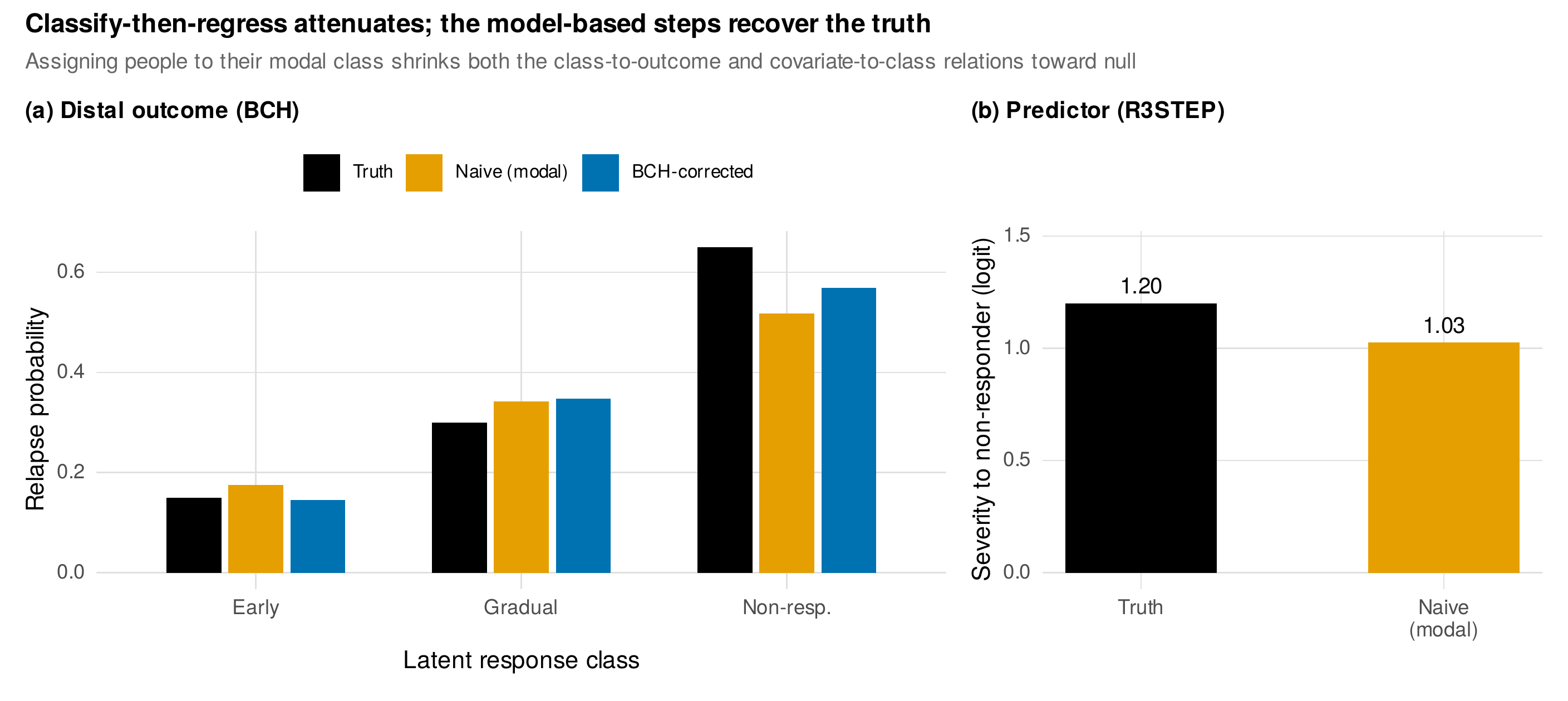
Note. On resp_classes: (a) the true relapse probabilities by class (black) are attenuated toward the average by modal assignment (orange) and pulled back by the BCH correction (blue). (b) the true log-odds of severity predicting non-responder membership (black) is attenuated under modal assignment (orange). The bias is modest at high entropy and grows as classification becomes uncertain.
22.5 Latent Transition Analysis
The models so far classify whole trajectories: a person belongs to one trajectory class for the entire study. A different categorical question asks not which trajectory type a person is but which status they occupy at each occasion, and how they move between statuses over time. A student might be engaged at one wave, ambivalent at the next, disengaged at a third; the object of interest is the sequence of statuses and the probabilities of transition between them. Latent transition analysis (LTA) formalizes this, and Collins and Lanza (2010) give its book-length treatment. It is built from a latent class measurement model at each wave, in which the status is inferred from a set of categorical indicators, joined across waves by a transition structure. Figure 22.8 draws the architecture: at each wave a latent status is measured by its indicators, and the statuses are linked by transition probabilities from one wave to the next.
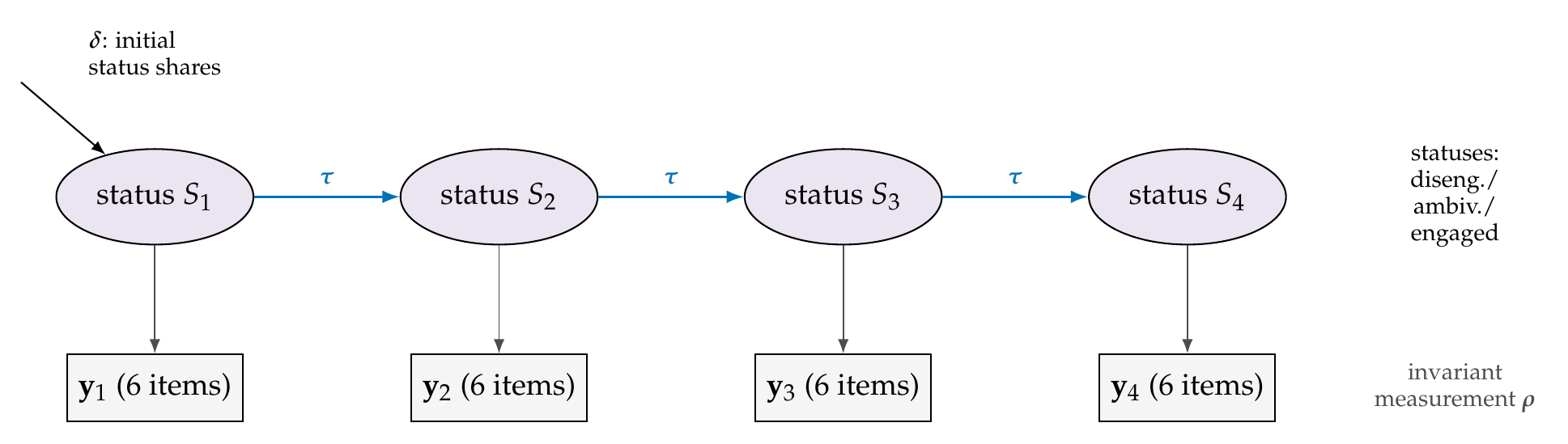
Note. At each wave the latent status \(S_w\) (one of three: disengaged, ambivalent, engaged) is measured by six binary indicators through status-specific, time-invariant item probabilities \(\bm{\rho}\). Initial status shares \(\bm{\delta}\) start the chain and the transition matrix \(\bm{\tau}\) links successive statuses. The structure is a hidden Markov model with a categorical measurement model and few occasions.
The model has three sets of parameters. The measurement parameters give the probability of endorsing each indicator conditional on status, and these should be held invariant across waves, the categorical echo of the longitudinal measurement invariance of Chapter 18: a status must mean the same thing at every occasion for a change in status to be interpretable rather than a change in what the status is. The initial-status parameters give the population shares of each status at the first wave. The transition parameters form a matrix whose entry in row \(a\), column \(b\) is the probability of moving to status \(b\) at the next wave given status \(a\) now; its diagonal is the probability of staying. Estimation is again by expectation-maximization, here the forward-backward recursion familiar from hidden Markov models, and it recovers the structure well. On the engage_status data, six binary engagement indicators measured over four waves with three planted statuses, the fitted model recovers the invariant item probabilities, the initial shares near their true values of \(0.30\), \(0.35\), and \(0.35\), and a transition matrix whose diagonal, near \(0.71\), \(0.65\), and \(0.73\), correctly reflects a mover-stayer structure in which most students keep their status from wave to wave. Table 22.5 is a glossary of the parameters and the invariance requirement.
Table 22.5. Latent transition analysis: parameters and requirements.
| Parameter | Meaning | Requirement or note |
|---|---|---|
| Item probabilities \(\bm{\rho}\) | Endorsement of each indicator given status | Hold invariant across waves so status meaning is stable |
| Initial shares \(\bm{\delta}\) | Status proportions at wave one | Sum to one |
| Transition matrix \(\bm{\tau}\) | \(P(\text{status at } w{+}1 \mid \text{status at } w)\) | Rows sum to one; diagonal is the staying probability |
| Mover-stayer variant | Some persons never move; others transition | A constrained transition structure |
| Number of statuses | Latent classes per wave | Chosen by the enumeration protocol, per wave |
Note. Invariance of the measurement parameters is the categorical counterpart of longitudinal measurement invariance (Chapter 18): without it, an apparent transition may be a change in what the status means rather than a change in the person.
Figure 22.9 shows the estimated transition matrix as a heatmap and the implied evolution of status prevalence over the four waves. The heatmap is dominated by its diagonal, the signature of a population of mostly stayers, with modest off-diagonal flow. Propagating the initial shares through the transition matrix shows the population composition drifting gently, here toward the ambivalent middle, as the small transitions accumulate. This is the interpretive payoff of the model: not a static classification but a description of movement, of how a population redistributes itself across statuses over time.
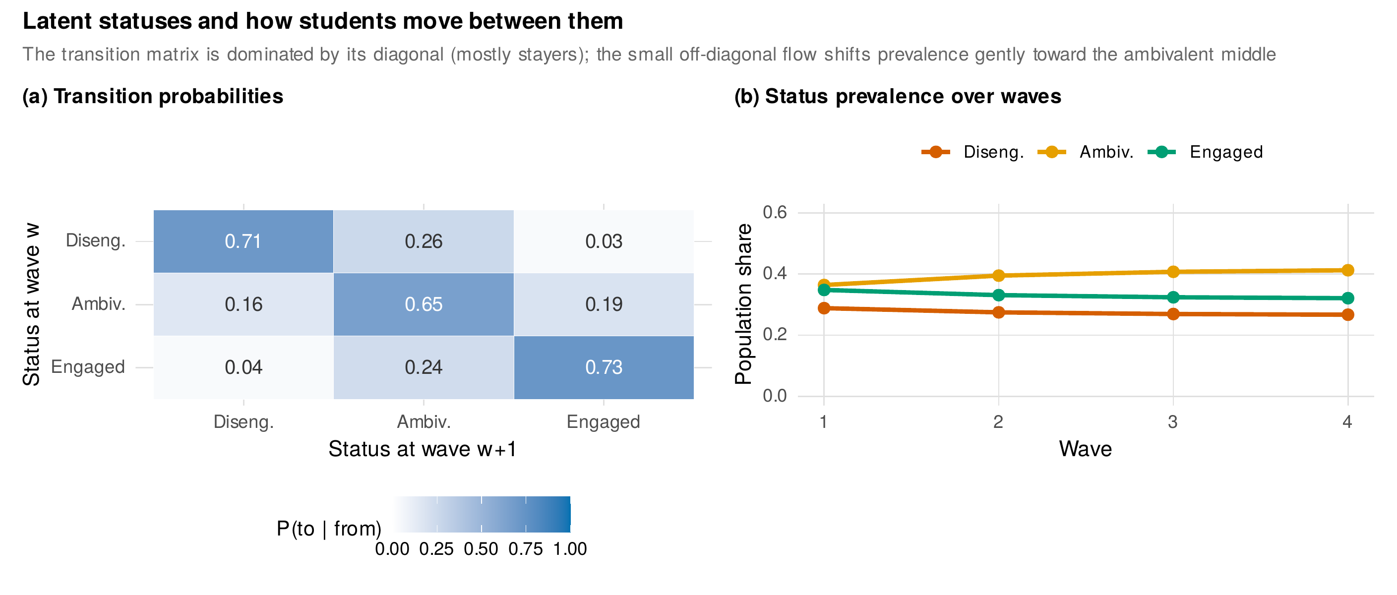
Note. Left: the estimated transition matrix from engage_status, dominated by its diagonal, the mark of a mostly-stayer population. Right: the population shares of each status across waves, obtained by propagating the initial shares through the transition matrix; the small off-diagonal flow shifts prevalence gently over time.
Latent transition analysis is, structurally, a hidden Markov model with a categorical measurement model and a small number of occasions, and the connection is worth naming because it locates LTA in a larger family. When the number of occasions is small, as in most panel studies, the LTA framing and its wave-specific interpretation are natural. When the series is long, the dynamic-systems framing of Chapters 24 and 26, where the same forward-backward machinery estimates the hidden states of an intensive single-subject or multi-subject series, becomes the more useful lens. The models are the same; the framing follows the design. The software box notes the R tools, depmixS4 and LMest among them, that estimate these models in practice.
Software Note • mixture and transition models in R and Mplus
The R ecosystem for these models is capable but uneven. Growth mixture and latent class growth models are fitted by lcmm (Proust-Lima, Philipps, & Liquet, 2017) and, for finite-mixture illustrations, mclust; latent class and profile models by poLCA and tidyLPA; latent transition and hidden Markov models by depmixS4 (Visser & Speekenbrink, 2010) and LMest (Bartolucci, Pandolfi, & Pennoni, 2017). Auxiliary-variable methods, R3STEP and BCH, have partial R coverage and remain most fully implemented in Mplus, whose workflow is scripted reproducibly from R through MplusAutomation. The computations in this chapter were carried out with expectation-maximization written from scratch, both because the mixture packages were unavailable in the build environment and because the from-scratch code makes the estimation transparent; the algorithms, the multi-start doctrine, the enumeration indices, and the forward-backward recursion for transitions are exactly those the packages implement. The shipped scripts are ch22_analysis_V01.R (the full toolkit), ch22_figures_V01.R, and the three generators gen_classes_sim_V01.R, gen_resp_classes_V01.R, and gen_engage_status_V01.R.
Common Pitfall • Five ways mixture analyses go wrong
First, choosing the number of classes from a single index, usually the BIC, when the decision is multi-criteria and the BLRT, class size, interpretability, and replication all bear on it. Second, interpreting modal-class assignments as error-free group memberships, then carrying them into downstream analyses that the misclassification attenuates. Third, enumerating classes without a covariate and then relating the classes to that covariate, without checking that the solution is stable when the covariate is included. Fourth, reifying a tiny class, two or three percent of the sample, as a substantively meaningful kind. Fifth, comparing LCGA and GMM class counts as if they were on the same scale, when LCGA’s zero-within-class-variance restriction systematically inflates the number of classes it needs.
22.6 Reporting and the Replication Imperative
The fragility of mixture results places an unusual weight on transparent reporting, and the field has responded with the GRoLTS checklist of van de Schoot and colleagues (2017), a set of guidelines for reporting latent trajectory studies that this chapter endorses and Table 22.6 adapts. The recurring themes are three. First, report the full solution path, not just the chosen model: the number of random starts, whether the best log-likelihood replicated, the fit indices across all \(K\) considered, and the reasons for the final choice. Second, plot the classes honestly. The most common mixture figure, clean mean curves one per class, is also the most misleading, because it hides the within-class spread and the classification uncertainty and makes the classes look crisper and more real than they are. The book standard, illustrated in Figure 22.10, overlays the member trajectories on the mean curves and shades each member by its classification certainty, so that the reader sees the fuzzy overlap between classes and the members the model is unsure about, not a tidy partition. Third, discipline the language. A mixture analysis licenses the statement that the data are consistent with a certain number of latent classes under stated assumptions; it does not license the claim that a certain number of kinds of people were discovered. The difference between those two sentences is the difference the whole chapter has been about.
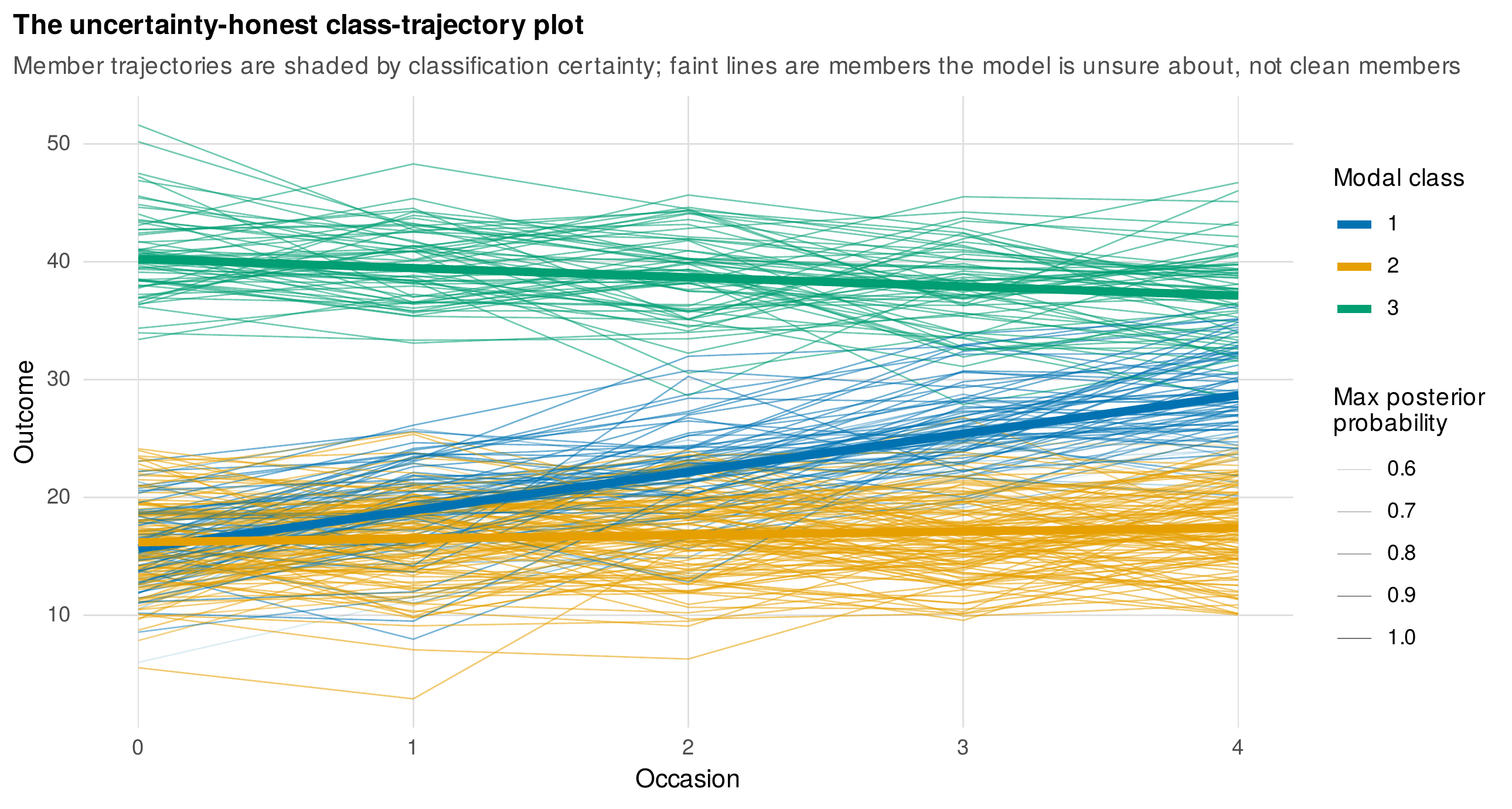
Note. Each member trajectory is drawn in its modal class color and shaded by the maximum posterior probability, so faint lines are members the model classifies with low confidence, not clean members of the class. The bold curves are the class means. This figure shows the overlap and the uncertainty that a mean-curves-only plot conceals, and it is the reporting standard this book enforces.
The resilience-classes literature is the cautionary case that makes the reporting standards concrete. Infurna and Luthar (2016) reexamined widely cited findings that a large majority of people are resilient to major life stressors, findings built on trajectory-class analyses, and showed that the resilient class was fragile to analytic choices and considerably smaller than claimed once the modeling was done carefully. The episode is not an argument against mixture models; it is an argument for the discipline this chapter has developed, because the difference between a robust finding and an artifact was exactly the difference between a careful multi-criteria enumeration with honest reporting and a single-index extraction with reified classes. Table 22.6 is the checklist that operationalizes the discipline.
Table 22.6. A GRoLTS-aligned reporting checklist for mixture models.
| Item | |
|---|---|
| 1 | Model type (LCGA vs. GMM) and the within-class variance specification, stated explicitly |
| 2 | Number of random starts and whether the best log-likelihood replicated, at every \(K\) |
| 3 | Fit indices (BIC, aBIC, CAIC), the BLRT, and entropy across all \(K\) considered, in a table |
| 4 | Smallest-class size and the substantive interpretability argument for the chosen \(K\) |
| 5 | Bauer-Curran probes: nonnormal-component checks, covariate-inclusion stability, continuous-model comparison |
| 6 | Replication evidence: split-half or independent-sample stability |
| 7 | Auxiliary-variable method (R3STEP, BCH) named, not classify-then-regress |
| 8 | An uncertainty-honest class-trajectory plot, not mean curves alone |
| 9 | Language that reports classes as consistent with the data, not as discovered kinds of people |
Note. Adapted from the GRoLTS checklist (van de Schoot et al., 2017). The items operationalize the chapter’s dual mandate: fit mixtures competently and report them with the skepticism their fragility demands.
Chapter Summary
Mixture models formalize the idea that a population contains categorically distinct subgroups of change, through latent class growth analysis, which fixes within-class variance to zero, and growth mixture modeling, which frees it; the restriction makes LCGA extract more classes than GMM, so their counts are not comparable. Estimation is by expectation-maximization from many random starts, and a best log-likelihood that does not replicate is a warning. Choosing the number of classes is a multi-criteria decision, information criteria, the bootstrap likelihood ratio test, entropy for classification quality only, class size, interpretability, and replication, never a single index. The governing caution is the Bauer-Curran result: a single nonnormal population yields spurious classes, because a mixture of normals approximates a skewed shape, so a well-fitting mixture is consistent with latent classes but does not establish them. Relating classes to covariates and outcomes requires three-step methods, R3STEP for predictors and BCH for distal outcomes, because assigning people to their modal class discards the classification uncertainty and attenuates every downstream relationship. Latent transition analysis models movement between statuses over time, a measured Markov chain with invariant categorical measurement, a transition matrix, and a hidden-Markov estimation that connects it to the dynamic models of later chapters. Reporting must follow the GRoLTS discipline: the full solution path, uncertainty-honest trajectory plots that show the overlap rather than clean mean curves, and language that reports classes as consistent with the data rather than as discovered kinds of people. Competence and skepticism are the same skill.
Exercises
- 22.1 Enumeration protocol. Run the full protocol of Table 22.3 on
classes_sim, whose true number of classes is three, assembling the information criteria, the bootstrap likelihood ratio test, entropy, and the split-half check, and document each step. - 22.2 Bauer-Curran lab. Analyze
classes_sim_skew, a single skewed population, with a normal growth mixture; show that the information criteria prefer more than one class, and write the temptation-and-resistance memo explaining why the classes are artifacts. - 22.3 LCGA versus GMM. Fit both an LCGA and a GMM to the same data and explain the discrepancy in the number of classes each prefers, in terms of the within-class variance restriction.
- 22.4 Auxiliary workflow. On
resp_classes, relate baseline severity to class membership and class to the relapse outcome, first by classify-then-regress and then by the model-based three-step logic, and quantify the attenuation the naive approach introduces. - 22.5 Latent transition. Fit a three-status latent transition model to
engage_status, recover the transition matrix, then refit with a planted violation of measurement invariance at one wave and show how it distorts the apparent transitions. - 22.6 GRoLTS audit. Given an excerpt from a published growth mixture paper, audit it against the checklist of Table 22.6 and write the reviewer comments its omissions warrant.
References
Asparouhov, T., & Muthén, B. (2014). Auxiliary variables in mixture modeling: Three-step approaches using Mplus. Structural Equation Modeling: A Multidisciplinary Journal, 21(3), 329–341. https://doi.org/10.1080/10705511.2014.915181
Bakk, Z., & Vermunt, J. K. (2016). Robustness of stepwise latent class modeling with continuous distal outcomes. Structural Equation Modeling: A Multidisciplinary Journal, 23(1), 20–31. https://doi.org/10.1080/10705511.2014.955104
Bartolucci, F., Pandolfi, S., & Pennoni, F. (2017). LMest: An R package for latent Markov models for longitudinal categorical data. Journal of Statistical Software, 81(4), 1–38. https://doi.org/10.18637/jss.v081.i04
Bauer, D. J. (2007). Observations on the use of growth mixture models in psychological research. Multivariate Behavioral Research, 42(4), 757–786. https://doi.org/10.1080/00273170701710338
Bauer, D. J., & Curran, P. J. (2003). Distributional assumptions of growth mixture models: Implications for overextraction of latent trajectory classes. Psychological Methods, 8(3), 338–363. https://doi.org/10.1037/1082-989X.8.3.338
Bauer, D. J., & Curran, P. J. (2004). The integration of continuous and discrete latent variable models: Potential problems and promising opportunities. Psychological Methods, 9(1), 3–29. https://doi.org/10.1037/1082-989X.9.1.3
Bolck, A., Croon, M., & Hagenaars, J. (2004). Estimating latent structure models with categorical variables: One-step versus three-step estimators. Political Analysis, 12(1), 3–27. https://doi.org/10.1093/pan/mph001
Collins, L. M., & Lanza, S. T. (2010). Latent class and latent transition analysis: With applications in the social, behavioral, and health sciences. Wiley. https://doi.org/10.1002/9780470567333
Grimm, K. J., Ram, N., & Estabrook, R. (2017). Growth modeling: Structural equation and multilevel modeling approaches. Guilford Press.
Infurna, F. J., & Luthar, S. S. (2016). Resilience to major life stressors is not as common as thought. Perspectives on Psychological Science, 11(2), 175–194. https://doi.org/10.1177/1745691615621271
Jung, T., & Wickrama, K. A. S. (2008). An introduction to latent class growth analysis and growth mixture modeling. Social and Personality Psychology Compass, 2(1), 302–317. https://doi.org/10.1111/j.1751-9004.2007.00054.x
Lanza, S. T., Tan, X., & Bray, B. C. (2013). Latent class analysis with distal outcomes: A flexible model-based approach. Structural Equation Modeling: A Multidisciplinary Journal, 20(1), 1–26. https://doi.org/10.1080/10705511.2013.742377
Masyn, K. E. (2013). Latent class analysis and finite mixture modeling. In T. D. Little (Ed.), The Oxford handbook of quantitative methods (Vol. 2, pp. 551–611). Oxford University Press. https://doi.org/10.1093/oxfordhb/9780199934898.013.0025
Moffitt, T. E. (1993). Adolescence-limited and life-course-persistent antisocial behavior: A developmental taxonomy. Psychological Review, 100(4), 674–701. https://doi.org/10.1037/0033-295X.100.4.674
Muthén, B., & Shedden, K. (1999). Finite mixture modeling with mixture outcomes using the EM algorithm. Biometrics, 55(2), 463–469. https://doi.org/10.1111/j.0006-341X.1999.00463.x
Nagin, D. S. (1999). Analyzing developmental trajectories: A semiparametric, group-based approach. Psychological Methods, 4(2), 139–157. https://doi.org/10.1037/1082-989X.4.2.139
Nylund, K. L., Asparouhov, T., & Muthén, B. O. (2007). Deciding on the number of classes in latent class analysis and growth mixture modeling: A Monte Carlo simulation study. Structural Equation Modeling: A Multidisciplinary Journal, 14(4), 535–569. https://doi.org/10.1080/10705510701575396
Nylund-Gibson, K., & Choi, A. Y. (2018). Ten frequently asked questions about latent class analysis. Translational Issues in Psychological Science, 4(4), 440–461. https://doi.org/10.1037/tps0000176
Nylund-Gibson, K., Grimm, R. P., & Masyn, K. E. (2019). Prediction from latent classes: A demonstration of different approaches to include distal outcomes in mixture models. Structural Equation Modeling: A Multidisciplinary Journal, 26(6), 967–985. https://doi.org/10.1080/10705511.2019.1590146
Proust-Lima, C., Philipps, V., & Liquet, B. (2017). Estimation of extended mixed models using latent classes and latent processes: The R package lcmm. Journal of Statistical Software, 78(2), 1–56. https://doi.org/10.18637/jss.v078.i02
Ram, N., & Grimm, K. J. (2009). Growth mixture modeling: A method for identifying differences in longitudinal change among unobserved groups. International Journal of Behavioral Development, 33(6), 565–576. https://doi.org/10.1177/0165025409343765
van de Schoot, R., Sijbrandij, M., Winter, S. D., Depaoli, S., & Vermunt, J. K. (2017). The GRoLTS-checklist: Guidelines for reporting on latent trajectory studies. Structural Equation Modeling: A Multidisciplinary Journal, 24(3), 451–467. https://doi.org/10.1080/10705511.2016.1247646
Vermunt, J. K. (2010). Latent class modeling with covariates: Two improved three-step approaches. Political Analysis, 18(4), 450–469. https://doi.org/10.1093/pan/mpq025
Visser, I., & Speekenbrink, M. (2010). depmixS4: An R package for hidden Markov models. Journal of Statistical Software, 36(7), 1–21. https://doi.org/10.18637/jss.v036.i07