Chapter 23
Multilevel Models for Diary and Intensive Longitudinal Data
This chapter opens Part VI, and with it a shift in the kind of data and the kind of question. The panel designs of Part V measured people a handful of times; intensive longitudinal designs measure them many times, several moments a day for days or weeks, through diaries, experience sampling, and ecological momentary assessment. The density of measurement makes a new question askable, and it is a within-person question: not how people who are more stressed differ from people who are less stressed, but how a person’s own affect moves on the occasions when they are more stressed than usual for them. The multilevel model of Chapter 13 is the instrument, redeployed here with the craft that dense within-person data demand: centering as the inferential centerpiece, now extended to lagged predictors; the nesting of moments in days in persons; the cycles that structure a day and a week; the trends that a fluctuation question must remove and a change question must model; the serial dependence that consecutive moments carry; and the mediation and moderation of processes as they unfold. This is, for many readers in social, personality, and clinical psychology, the destination chapter, the one their own data most resembles, so it is written to stand alone. It also marks a boundary. The multilevel model treats the dynamics as nuisance to be tidied; when the dynamics themselves become the question, when the estimand is how a system carries itself forward, the tools of Chapters 24 through 28 take over, and this chapter closes by marking exactly where that handoff falls.
Learning Objectives
After working through this chapter, you should be able to: (1) translate a within-person process question into a multilevel specification and read its random slopes as individual differences in the process; (2) execute the centering doctrine with lagged predictors and interpret within-person, between-person, and contextual effects in intensive-longitudinal terms; (3) choose among two-level, three-level, and cross-classified structures from design and intraclass-correlation evidence; (4) model diurnal and weekly cycles with sine-cosine terms, reconstruct their amplitude and phase, and allow person-varying rhythms; (5) decide, by estimand, whether to detrend or model a trend, and recognize trend leakage; (6) handle serial dependence at level one, distinguishing an AR(1) residual structure from a lagged-outcome specification and their different estimands and biases; (7) estimate a within-person 1-1-1 mediation with its random-effect covariance term and correct uncertainty; and (8) write a complete, reviewer-proof diary-study results section.
23.1 Process Questions and the Within-Person Regression
The defining move of intensive longitudinal analysis is to ask a question inside the person. Consider stress and negative affect. A between-person question asks whether people who report more stress also report more negative affect, a fact about how persons rank against one another. A within-person question asks whether a given person feels worse on the occasions when they are more stressed than is typical for them, a fact about how that person’s states move together over time. The two are logically distinct, they can even have opposite signs, and the whole apparatus of Chapter 13’s centering exists to keep them apart. Person-mean centering a momentary predictor, subtracting each person’s own average stress from each of their momentary reports, isolates the within-person deviation, and a regression on that deviation answers the within-person question directly. The person means, entered separately, carry the between-person information. This disaggregation, developed for panel data by Curran and Bauer (2011) and by Wang and Maxwell (2015), codified for centering by Enders and Tofighi (2007), Hoffman and Stawski (2009), and Hamaker and Muthén (2020), is the same doctrine as Chapter 13.4, now the daily bread of a chapter where every predictor is measured repeatedly within the person. The analysis of such data has a long methodological lineage, from the early treatment of daily-experience data by West and Hepworth (1991) to the experience-sampling handbook of Hektner, Schmidt, and Csikszentmihalyi (2007).
Figure 23.1 makes the within-person question visible. Each panel is one person’s own regression of momentary negative affect on their person-centered momentary stress, twelve people from the ema_stress data, a two-week experience-sampling study with six beeps a day in 120 people. The slopes differ, plainly. One person’s affect climbs steeply with their stress; another’s barely moves; a third’s, at the floor of the scale, is flat. That variation is not noise around a common slope to be averaged away. It is the phenomenon: people differ in how reactive their affect is to their own stress, and a model that only reported the average slope would discard the most interesting thing in the data. This is the substantive reading of a random slope, developed in the personality-process tradition of Bolger and Zuckerman (1995) and the daily-stress work of Bolger, DeLongis, Kessler, and Schilling (1989): the random slope’s variance is an individual-differences finding, and its explanation by person-level covariates is the next question.
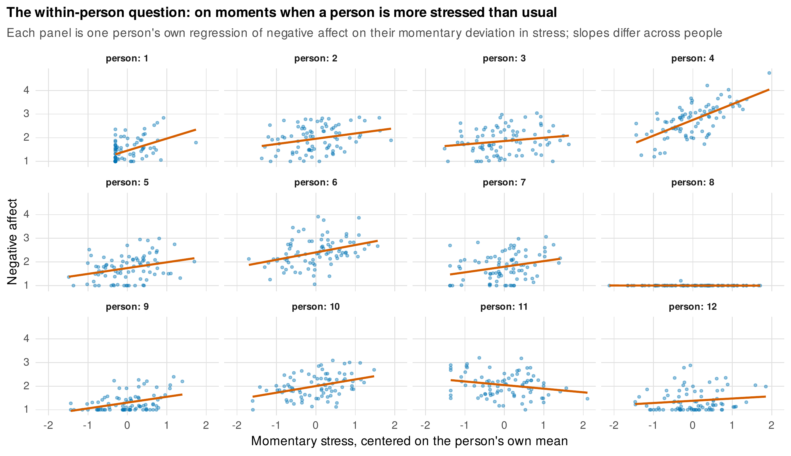
Note. Each panel regresses one person’s momentary negative affect on their person-centered momentary stress, for twelve people from ema_stress. The slopes differ across people: some are steeply reactive, others nearly flat. That heterogeneity, not the average slope alone, is the object of study.
The multilevel model formalizes this. Writing \(\mathrm{na}_{it}\) for person \(i\)’s negative affect at occasion \(t\) and \(\mathrm{stress}^{wc}_{it}\) for their person-centered stress, the model \(\mathrm{na}_{it} = \beta_{0i} + \beta_{1i}\,\mathrm{stress}^{wc}_{it} + \gamma_2\,\overline{\mathrm{stress}}_i + e_{it}\), with \(\beta_{0i}\) and \(\beta_{1i}\) random across persons, estimates an average within-person reactivity in the fixed slope and its heterogeneity in the slope variance. Fitted to ema_stress, the average within-person stress reactivity is \(0.27\) on the affect scale, and the random-slope standard deviation is substantial, so people range from essentially unreactive to strongly reactive. Figure 23.2 shows the distribution of the person-specific reactivities and the two people at its extremes, one whose affect tracks their stress closely and one whose does not. The spread is the finding.
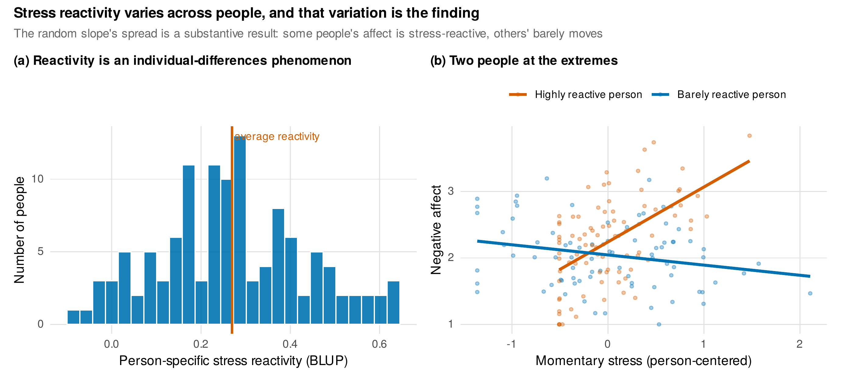
Note. (a) The distribution of person-specific stress reactivities (best linear unbiased predictors) from the random-slope model on ema_stress; the line marks the average. (b) The most and least reactive people: one person’s negative affect climbs with their momentary stress, the other’s is nearly flat. The variation across people is a substantive result, not statistical insurance.
Once reactivity is recognized as varying, the question becomes what explains it, and the answer is a cross-level interaction: a person-level covariate that moderates the within-person slope. In ema_stress, neuroticism plays this role. Adding the interaction of person-centered stress with neuroticism, \(\beta_{1i} = \gamma_{10} + \gamma_{11}\,\mathrm{neuroticism}_i + u_{1i}\), estimates \(\gamma_{11}=0.13\) (\(SE=0.01\)): more neurotic people are more reactive to their own stress. Figure 23.3 probes the interaction by plotting the predicted within-person slope across the range of neuroticism with its confidence band, the person-specific reactivities scattered around it. The cross-level interaction has explained part of the slope variance, turning a described heterogeneity into a modeled one. The grammar of these specifications, from question to formula, is collected in Table 23.1.
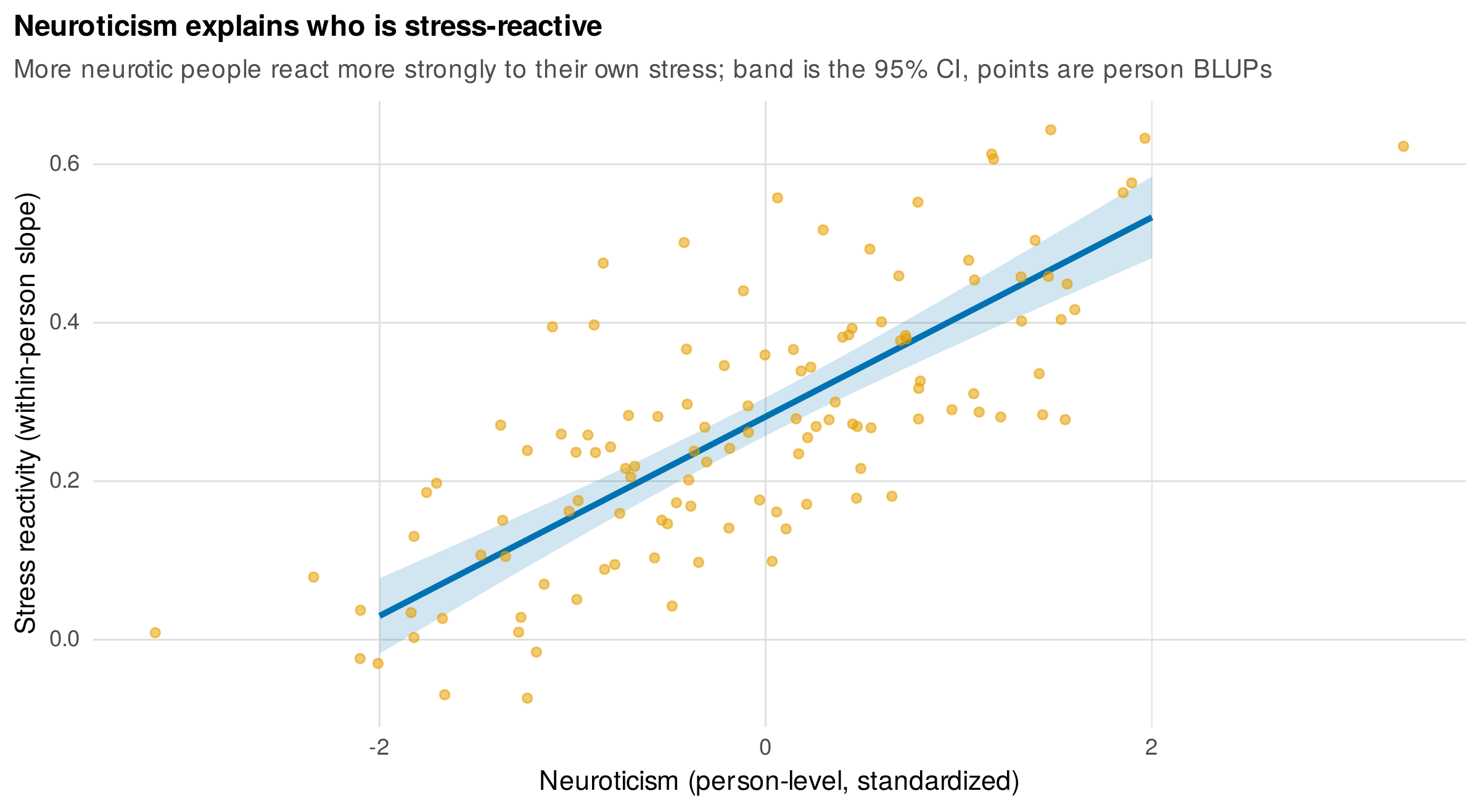
Note. The predicted within-person stress-reactivity slope rises with neuroticism (line with 95% confidence band); points are the person-specific reactivities. The cross-level interaction explains part of the heterogeneity in reactivity that Figure 23.2 displayed.
Table 23.1. From process question to multilevel specification.
| Question (the “on occasions when” grammar) | Specification |
|---|---|
| On occasions when a person is more stressed than usual, is their affect worse? | Person-center stress; regress affect on the within-person deviation with a random intercept |
| Do people differ in that reactivity? | Add a random slope for the within-person predictor |
| Who is more reactive? | Add a cross-level interaction (person covariate \(\times\) within predictor) |
| Is there a between-person association too? | Enter the person mean of the predictor separately |
| Does yesterday’s state carry into today? | Add a lagged predictor or outcome (Section 23.5) |
Note. The within-person deviation answers the process question; the person mean carries between-person information; the random slope and its moderators carry the individual differences. Centering is what keeps these separate.
23.2 Structure: How Many Levels Does the Design Create?
An intensive design nests observations in a hierarchy, and the analyst must decide how many levels to model. Beeps are nested in persons, giving the two-level structure used above; but beeps are also nested in days, and days in persons, giving a three-level structure; and because the same time-of-day slots recur across days, beeps are cross-classified by person and by slot. Figure 23.4 draws the three. The decision is not merely technical, because a day-level random effect represents something real, a person’s day being better or worse as a whole, above the momentary fluctuations within it, and ignoring it when it is present understates the clustering and can distort inference. The evidence for how many levels are needed is the same intraclass-correlation logic of Chapter 7, applied now to the extra day level.
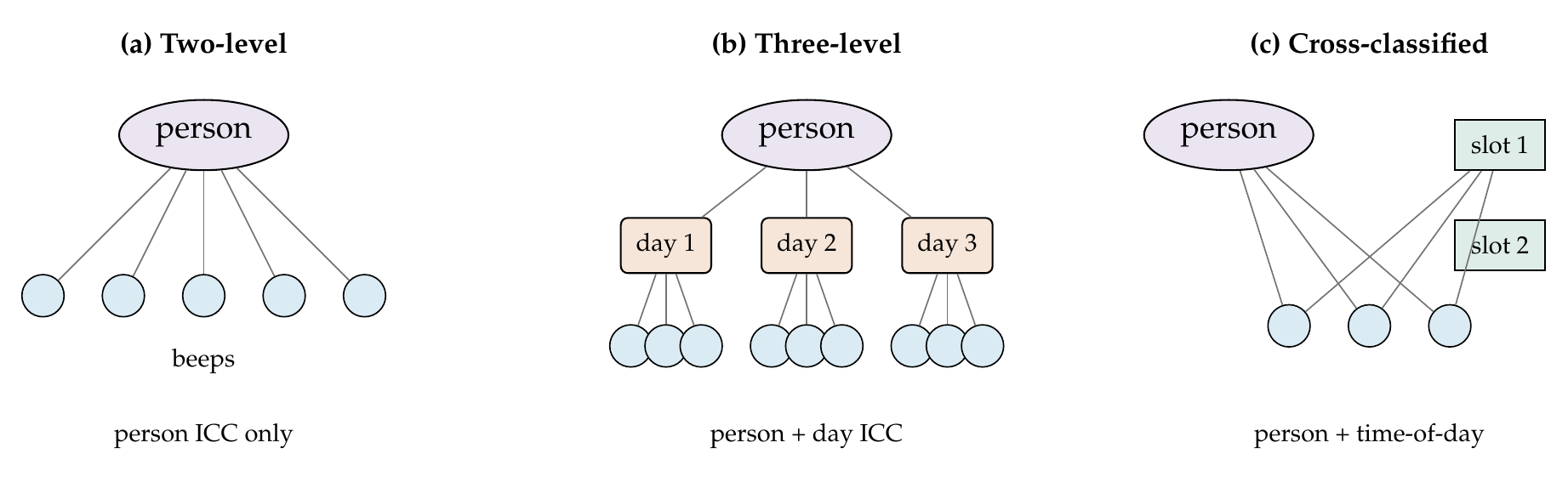
Note. Beeps (blue circles) may be modeled as nested in persons only (a); as nested in days within persons (b), which adds a day-level random effect for whole-day highs and lows; or as cross-classified by person and by recurring time-of-day slot (c). The intraclass correlations at each level, estimated from a null model, guide the choice.
On ema_stress, a null three-level model partitions the variance of negative affect into a person share, a day-within-person share, and a beep-level share. The person intraclass correlation is \(0.42\), so a large part of the variance is stable between-person difference, the reason centering matters. The additional day-level share is \(0.06\), modest but nonzero: days do cluster the beeps within them, and a three-level model captures that a person’s Tuesday can be worse than their Wednesday as a whole. Whether to carry the third level is a judgment balancing this evidence against parsimony and convergence, and Table 23.2 lays out the decision. The related question of whether a predictor lives at the moment level or the day level, a momentary stress report versus a day’s aggregated stress, is a construction choice of the kind Chapter 5 raised: aggregating momentary reports to a daily mean creates a day-level predictor with its own between-day and within-day parts, and the aggregation should be deliberate, not accidental.
Table 23.2. Choosing the level structure.
| Design feature | Evidence | Structure |
|---|---|---|
| Beeps within persons only, no day grouping of interest | Person ICC substantial; day ICC near zero | Two-level (beeps in persons) |
| Whole-day highs and lows plausible | Nonzero day-level ICC in a null three-level model | Three-level (beeps in days in persons) |
| Recurring time-of-day slots share variance across persons | Slot-level clustering | Cross-classified (person \(\times\) slot) |
| Day-level predictors of interest | Predictor defined per day | Aggregate to day level, decompose |
Note. The intraclass correlations from a null model are the primary evidence. A near-zero day-level ICC argues for the simpler two-level model; a nonzero one, and substantive interest in whole-day effects, argues for three levels. Convergence economics (the practice box) also bear on the choice.
23.3 Time Within the Day and Week: Cycles
Affect is not flat across a day. It has a rhythm, rising or falling with the hours, and that diurnal cycle is either a nuisance to be removed or a phenomenon to be studied, but either way it must be modeled or it will contaminate everything else. The standard tool is trigonometric regression: a sine-cosine pair at the daily period, \(\beta_c\cos(2\pi\,h/24) + \beta_s\sin(2\pi\,h/24)\) where \(h\) is the hour, which represents a smooth cycle with two coefficients. The pair is more interpretable than it looks, because it reconstructs to an amplitude and a phase: the amplitude \(\sqrt{\beta_c^2+\beta_s^2}\) is the size of the swing from the daily mean to the peak, and the phase \(\arctan(\beta_s/\beta_c)\) locates the peak in the day. The foundations box gives the algebra and the delta-method confidence interval. On ema_stress, the fitted cosine and sine coefficients are \(0.23\) and \(0.12\), reconstructing to an amplitude of \(0.26\) (\(SE=0.01\)), with negative affect lowest around midday and rising across the afternoon toward an evening peak. Figure 23.5 draws the fitted rhythm and its amplitude, and a gallery of person-specific rhythms.
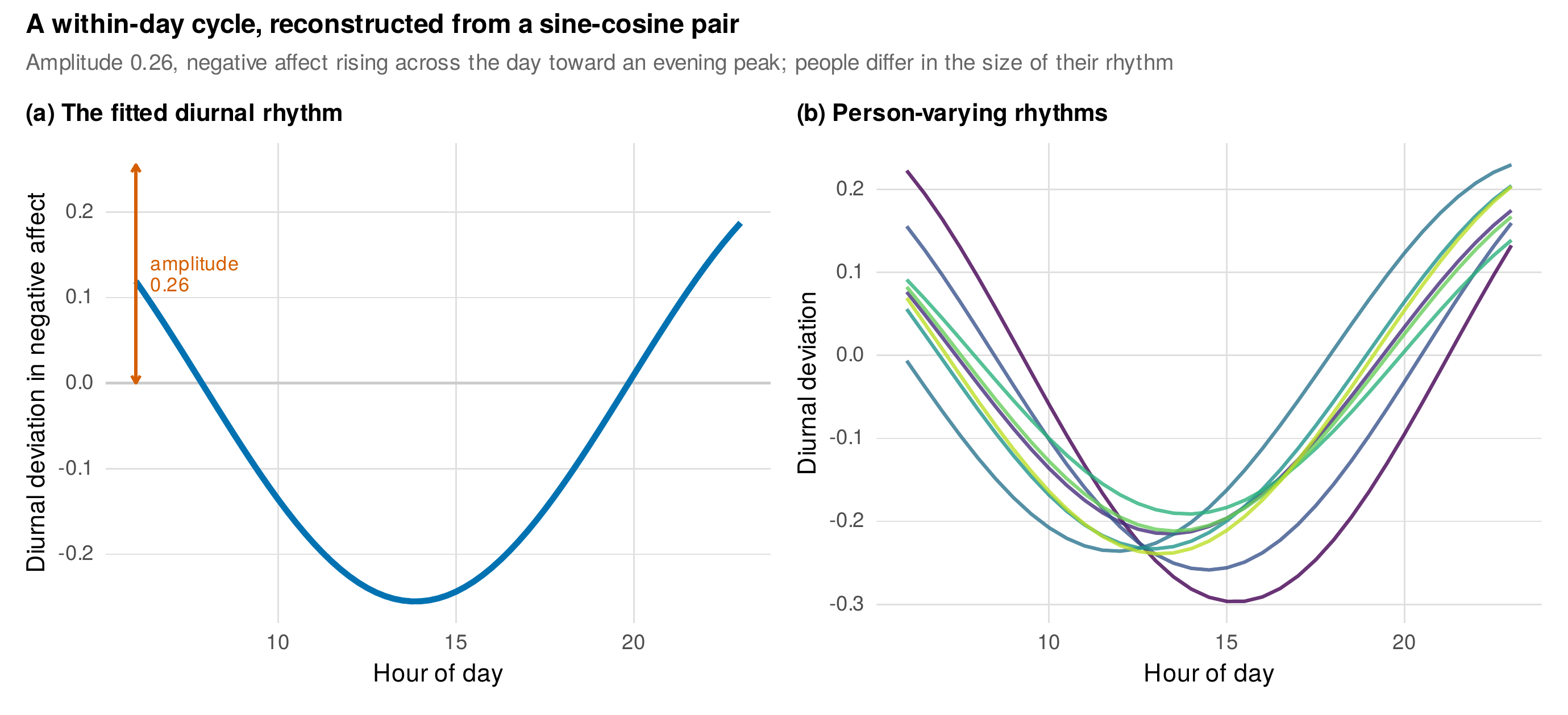
Note. (a) The population diurnal rhythm from a sine-cosine pair, amplitude \(0.26\): negative affect dips at midday and rises toward evening. (b) Person-varying rhythms from random sine and cosine coefficients; people differ in the size and shape of their daily swing. Amplitude and phase are reconstructed from the two trigonometric coefficients.
Foundations Box • Amplitude and phase from a sine-cosine pair; the mediation covariance term
A daily cycle written as \(\beta_c\cos\theta + \beta_s\sin\theta\) with \(\theta = 2\pi h/24\) is equivalent to \(A\cos(\theta-\phi)\) with amplitude \(A=\sqrt{\beta_c^2+\beta_s^2}\) and phase \(\phi=\arctan_2(\beta_s,\beta_c)\), so the two regression coefficients encode the height and timing of one smooth peak per day. The amplitude’s standard error follows from the delta method: with gradient \((\beta_c/A,\ \beta_s/A)\) and the coefficients’ covariance matrix \(\mathbf{V}\), \(\widehat{SE}(A)=\sqrt{\mathbf{g}^\top\mathbf{V}\mathbf{g}}\). Random person-specific sine and cosine coefficients give person-varying amplitude and phase. A separate algebra governs multilevel mediation. When the \(a\)-path (predictor to mediator) and the \(b\)-path (mediator to outcome) both vary randomly across persons, the average within-person indirect effect is not \(a\,b\) but \(a\,b + \mathrm{cov}(a_i,b_i)\): the covariance of the two random slopes adds to the product of their means (Bauer, Preacher, & Gil, 2006). Omitting the covariance term biases the indirect effect, and it is the most frequently forgotten quantity in multilevel mediation.
Whether the cycle is nuisance or phenomenon depends on the question. If the interest is in stress reactivity and the diurnal rhythm is merely a source of variance that would otherwise inflate the residual and confound a predictor that also varies with time of day, the cycle is partialled out and forgotten. If the interest is in the rhythm itself, in chronotype, in whether some people’s affect peaks in the morning and others’ at night, the person-varying amplitude and phase are the estimands. A weekly cycle deserves the same care: negative affect can run lower on weekends, a weekday-weekend contrast or a day-of-week factor captures it, and Liu and West (2016) warn that an unmodeled weekly cycle is a common oversight in daily-diary data. In ema_stress the weekend effect on negative affect is \(-0.06\). Table 23.3 is the menu of cycle specifications.
Table 23.3. A menu for modeling cycles.
| Goal | Specification | Reconstruction |
|---|---|---|
| Fixed diurnal cycle | \(\beta_c\cos\theta + \beta_s\sin\theta\), \(\theta=2\pi h/24\) | \(A=\sqrt{\beta_c^2+\beta_s^2}\), \(\phi=\arctan_2(\beta_s,\beta_c)\) |
| Person-varying rhythm | Random \(\cos\theta\) and \(\sin\theta\) slopes | Per-person amplitude and phase |
| Two harmonics (twice-daily) | Add \(\cos 2\theta\), \(\sin 2\theta\) | Second-harmonic amplitude |
| Weekday and weekend | Weekend indicator or day-of-week factor | Weekly contrast |
| Cycle by covariate | Interact trig terms with a covariate | Covariate-varying rhythm |
Note. Trigonometric terms give a smooth, few-parameter cycle whose amplitude and phase are recoverable; a factor for day-of-week is a less smooth alternative. Whether cycles are partialled as nuisance or estimated as phenomenon is set by the research question.
23.4 Trends: The Fluctuation-Versus-Change Fork
Over two weeks a person’s affect may drift, and that trend forces a decision that turns entirely on the estimand. If the question is about fluctuation, about how a person’s affect moves around their own level on the occasions when they are stressed, then a trend is a contaminant: it inflates the within-person variance and, worse, it can leak into the within-person effect if the predictor also trends. If the question is about change, about how the person’s level itself evolves, then the trend is the signal and must be modeled, often in a growth-and-process hybrid that carries both a trajectory and within-person fluctuations around it. The wording of this fork is coordinated deliberately with the time-varying-covariate treatment of Chapter 14.4 and the dynamic models of Chapter 25, because it is one doctrine appearing at three sites.
The leakage is worth seeing. Figure 23.6 simulates a within-person predictor that trends over time and an outcome that depends on the predictor’s fluctuation and carries its own trend. When the predictor is person-mean centered in the usual way, the centered deviation still contains the trend, and the trend in the outcome correlates with it, so the estimated within-person effect is inflated, \(0.38\) against a true value of \(0.30\). Person-specific detrending, regressing out each person’s linear trend before forming the within-person deviation, recovers the truth at \(0.30\). The lesson is that person-mean centering assumes stationarity, and when a trend is present the centering must be preceded by detrending, or the trend must be entered as a covariate, or the within-person effect will absorb it. Table 23.4 states the fork.
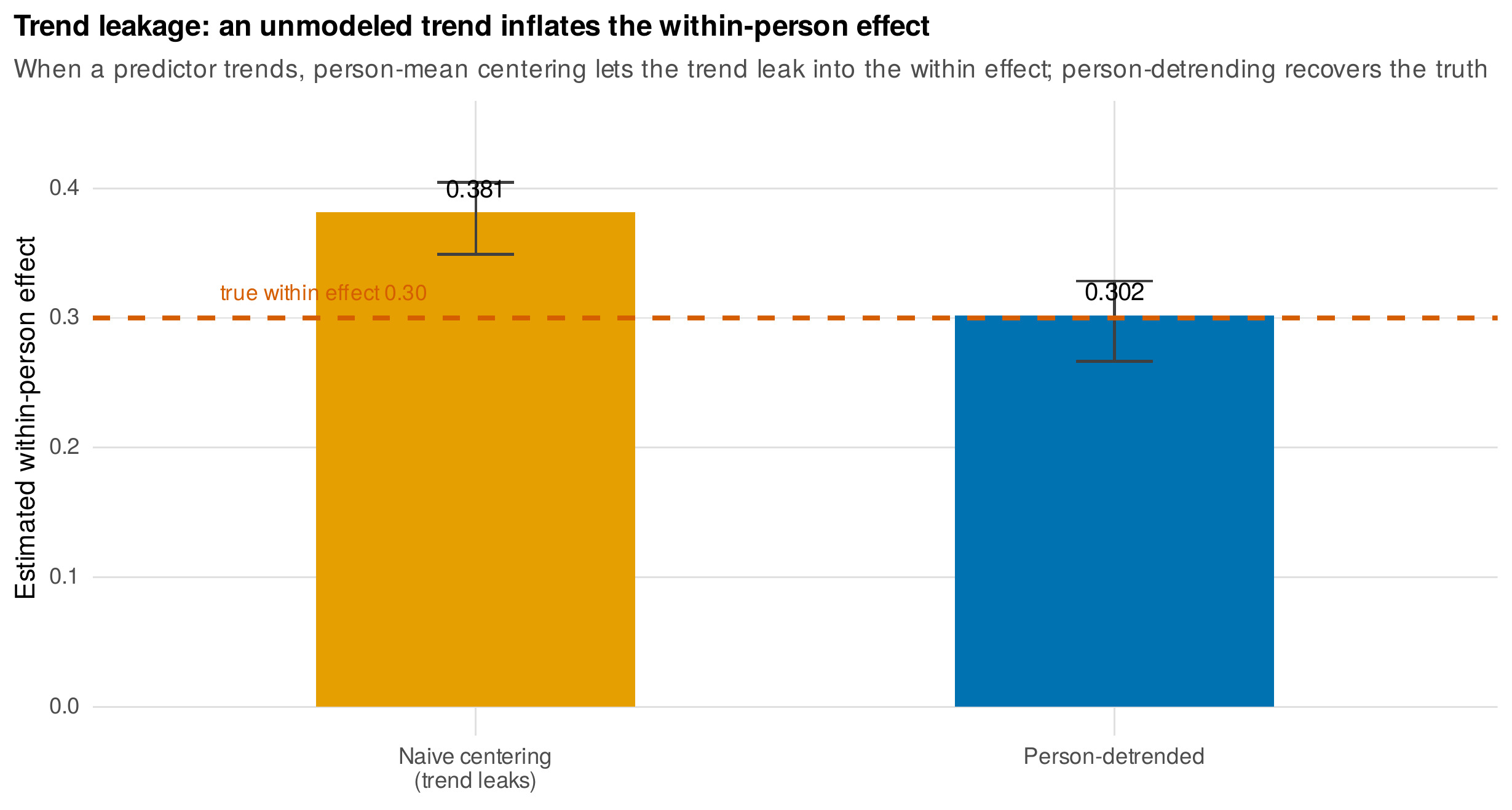
Note. When a within-person predictor trends over time, naive person-mean centering lets the trend leak into the within-person effect, inflating it above its true value of \(0.30\). Person-specific detrending before centering recovers the truth. Bars are means over simulated samples; whiskers are the 2.5th-to-97.5th percentiles.
Table 23.4. The trend fork: fluctuation versus change.
| Estimand | Approach | Consequence of the wrong choice |
|---|---|---|
| Within-person fluctuation | Detrend per person (linear or spline), then center; or enter time as a covariate | Leaving a trend in inflates or distorts the within-person effect |
| Within-person change | Model the trend (growth curve plus within-person process) | Detrending removes the very signal of interest |
| Both | Growth-and-process hybrid: trajectory plus centered fluctuations | Conflating them mixes level change with momentary reactivity |
Note. The choice is dictated by the question, not by the data. A fluctuation question requires a stationary within-person series, so a trend is removed; a change question requires the trend, so it is modeled. Coordinated with Chapters 14.4 and 25.
23.5 Yesterday Matters: Lags and Serial Dependence
Consecutive moments are not independent. A person feeling bad now tends to feel bad shortly after, and this serial dependence at level one must be handled, but how to handle it is a genuine fork with two branches that answer different questions and carry different biases. The first branch treats the dependence as a property of the residuals: the within-person errors are autocorrelated, an AR(1) structure in which \(e_{it}=\rho\,e_{i,t-1}+\text{noise}\), and modeling it corrects the standard errors of the within-person effects without changing their meaning. The within-person reactivity remains the estimand; the AR(1) simply acknowledges that the process noise is not white. On ema_stress, an AR(1) residual structure fitted by generalized least squares estimates the autocorrelation at \(0.30\), and Figure 23.8 shows that the residual autocorrelation, clearly present in a model that ignores it, is whitened once the AR(1) is included. The second branch puts the prior state into the mean model as a lagged outcome, regressing current affect on its own previous value, which changes the estimand: the coefficients are now conditional on the prior state, and the lagged-outcome coefficient is itself a substantive quantity, the carryover or inertia of affect. Figure 23.7 diagrams the two, and Table 23.5 states when each is preferred.
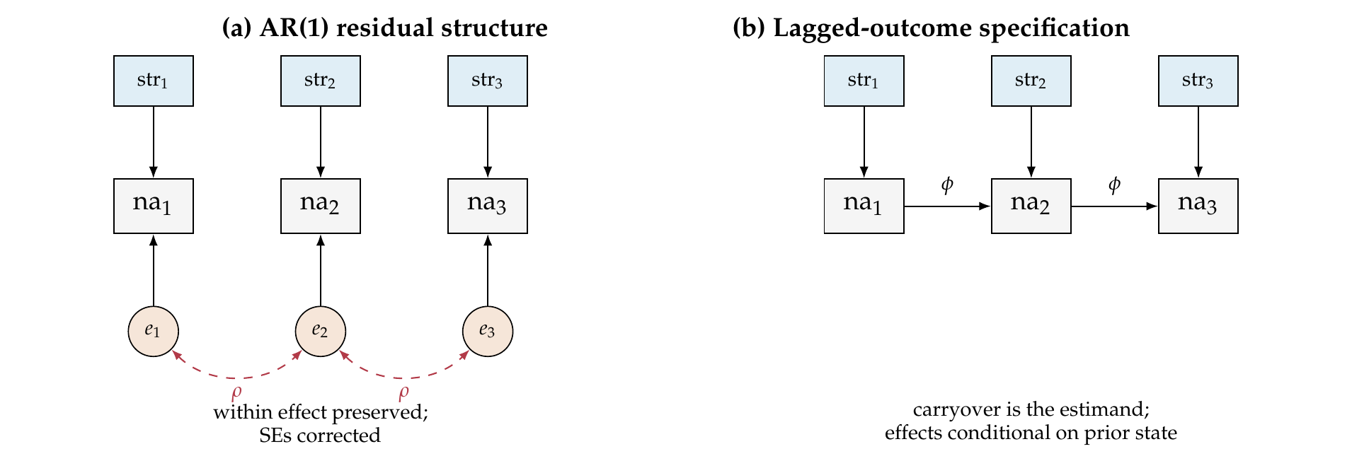
Note. (a) An AR(1) residual structure treats the within-person errors as autocorrelated (\(\rho\)); the within-person reactivity is unchanged and its standard errors are corrected. (b) A lagged-outcome specification puts the prior affect into the mean model (\(\phi\)); the carryover becomes the estimand and all effects become conditional on the prior state. The two answer different questions.
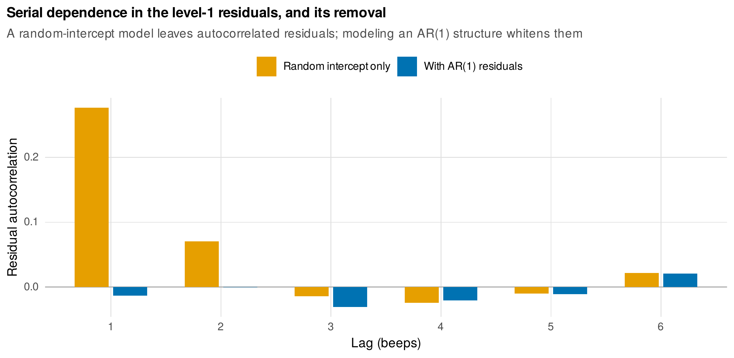
Note. The autocorrelation of the level-1 residuals from a random-intercept model on ema_stress (orange) shows the AR(1) signature: a lag-1 correlation near \(0.28\) decaying over lags. Modeling an AR(1) residual structure whitens them (blue). This diagnostic belongs in every intensive-longitudinal report.
The lagged-outcome branch carries a hazard that must be stated plainly. Regressing current affect on its prior value while also including a person random intercept produces a biased carryover coefficient when the number of occasions per person is small, because the random intercept is correlated with the lagged outcome and cannot be estimated well from few observations. Figure 23.9 quantifies it by simulation: with a true carryover of \(0.40\), the random-intercept estimate is inflated to \(0.62\) at five occasions and only settles onto the truth as the occasions grow into the dozens. This is the multilevel cousin of the Nickell (1981) bias met in Chapter 21, where the fixed-effects version of the same estimator was biased in the opposite, downward direction; neither is trustworthy at small \(T\), and McNeish and Stapleton (2016) survey the small-sample corrections. The honest conclusion is that a lagged-outcome model needs many occasions per person, and that when the dynamics are the real interest the dynamic structural equation models of Chapter 25 estimate them properly. Within the range where a lagged-outcome model is defensible, it earns its keep on genuinely dynamic questions: does today’s conflict predict tomorrow’s mood controlling for today’s mood, the cross-day carryover contrasts that are the signature analyses of the Bolger and Laurenceau (2013) and Laurenceau, Barrett, and Pietromonaco (1998) tradition. Figure 23.10 shows the same-day and lagged effects side by side on ema_stress: momentary stress moves affect strongly in the moment, the carryover of affect is substantial, and the lagged stress effect, conditional on the prior state, is small and even slightly negative, a reminder that lagged and contemporaneous effects are different quantities.
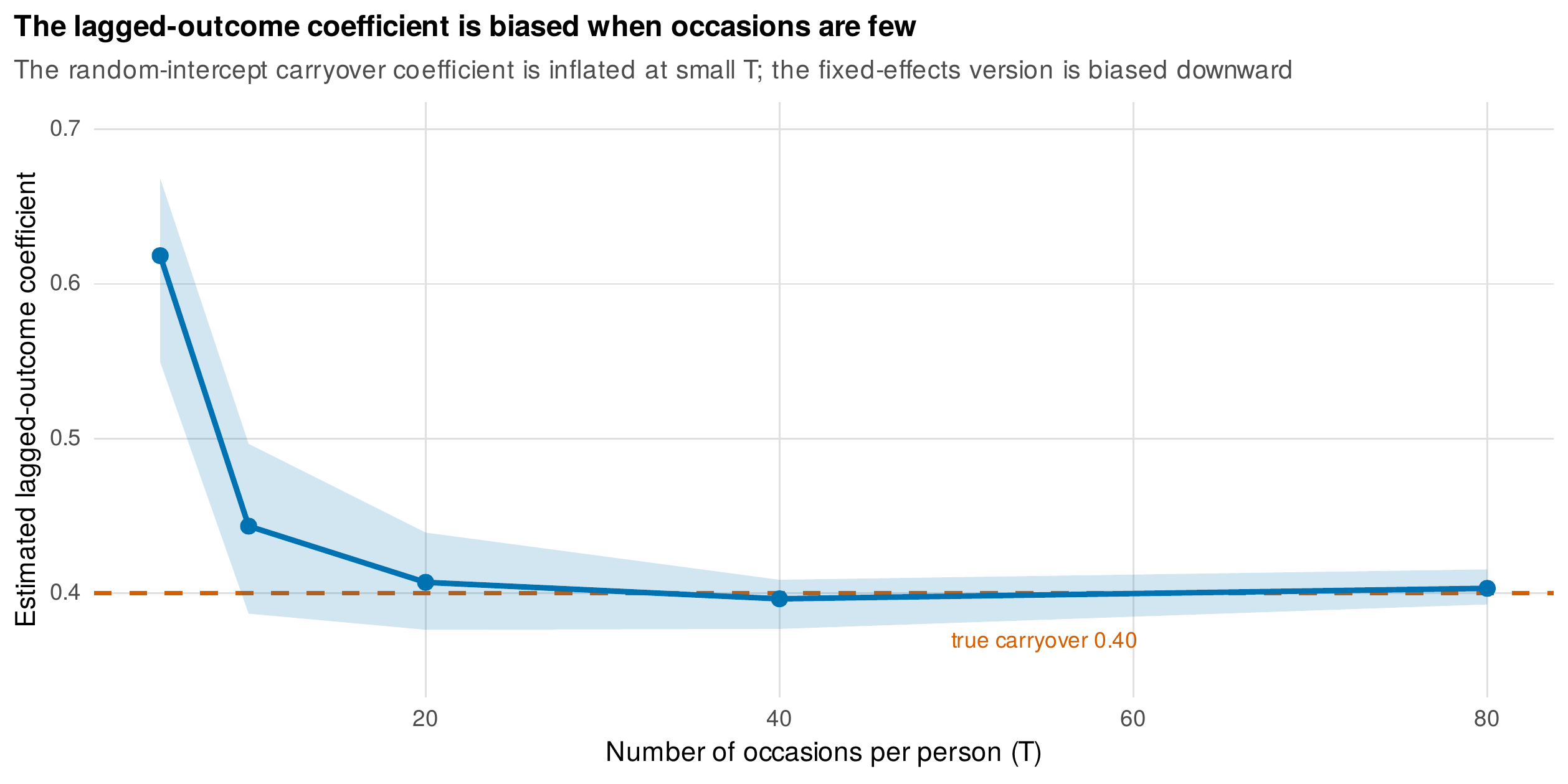
Note. With a true carryover coefficient of \(0.40\), the random-intercept lagged-outcome estimate is inflated when occasions per person are few and settles onto the truth only as the number grows. The fixed-effects version of the same estimator is biased downward (Chapter 21). Below Chapter 25’s tools, both mislead at small \(T\).
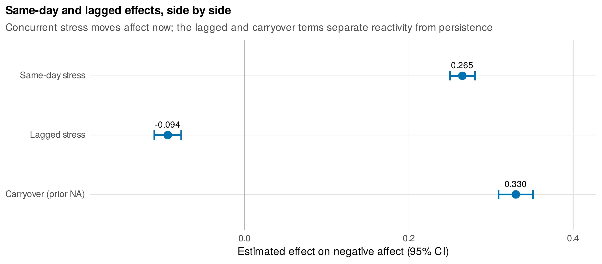
Note. On ema_stress: momentary stress moves negative affect strongly within the occasion; prior affect carries over substantially; and the lagged stress effect, conditional on the prior state, is small and slightly negative. Separating same-day from lagged effects is a signature intensive-longitudinal analysis.
Table 23.5. The serial-dependence fork.
| Approach | Estimand | Bias risk | When preferred |
|---|---|---|---|
| AR(1) residuals | Within-person reactivity, unchanged | None added; SEs corrected | Dependence is nuisance; reactivity is the question |
| Lagged outcome | Carryover; effects conditional on prior state | Small-\(T\) bias (up with random, down with fixed intercept) | Carryover is the substantive question; many occasions |
| Full dynamic model (Ch. 25) | Person-specific dynamics | Proper treatment | Dynamics are the estimand |
Note. The choice is by estimand, not fit. If the dependence is a nuisance and reactivity is the question, model it as AR(1) residuals. If carryover is the question, use a lagged outcome, but only with enough occasions, and hand off to Chapter 25 when the dynamics themselves are the target.
23.6 Within-Person Mediation and Moderation
A process question often has a mechanism: stress raises rumination, and rumination raises negative affect, a chain in which all three variables are measured repeatedly within the person, a 1-1-1 mediation. The multilevel apparatus estimates it, but with a subtlety that is the single most common error in the area. The \(a\)-path from stress to rumination and the \(b\)-path from rumination to affect both vary across persons, and when two random slopes are multiplied their expected product is not the product of their means but the product plus their covariance: the average within-person indirect effect is \(a\,b + \mathrm{cov}(a_i,b_i)\). Omitting the covariance term, as a naive two-model approach does, biases the indirect effect. The remedy of Bauer, Preacher, and Gil (2006) is a single stacked multilevel model that estimates both equations jointly and allows the \(a\)- and \(b\)-path random effects to covary, from which the covariance term is read directly. Figure 23.11 draws the 1-1-1 model with its random paths.
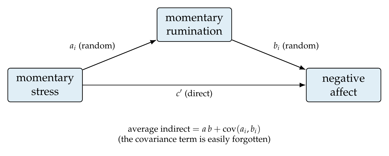
Note. All three variables are measured repeatedly within the person. The \(a\)-path (stress to rumination) and \(b\)-path (rumination to affect) vary randomly across persons, so the average within-person indirect effect is \(a\,b + \mathrm{cov}(a_i,b_i)\), the product of the average paths plus their covariance. The direct path \(c'\) is the reactivity net of the mediated route.
Fitted to ema_stress as a stacked model, the \(a\)-path is \(0.34\), the \(b\)-path is \(0.23\), and the direct path is \(0.19\); the fixed indirect effect \(a\,b\) is \(0.076\) with a Monte Carlo 95% confidence interval of \([0.062, 0.091]\), and the estimated \(a\)-\(b\) covariance adds a further \(0.006\), so the total average indirect effect is \(0.081\). The Monte Carlo interval, drawing the two paths from their joint sampling distribution and taking the percentiles of their product, is the appropriate uncertainty for an indirect effect, whose sampling distribution is not normal; the same logic as Chapter 21’s mediation, here inside persons. A Bayesian implementation, in the manner of Vuorre and Bolger (2018), handles the random covariance and the interval in one step and is often the cleanest route when the software is available. The multilevel structural equation framework of Preacher, Zyphur, and Zhang (2010) is the other principled option, separating the within- and between-person parts of the mediation explicitly. Within-person moderation, the interaction of two within-person predictors, follows the same centering discipline: both predictors are person-centered, and their product is formed from the centered versions, or the interaction will conflate within- and between-person effects.
23.7 The Complete Worked Study and Reporting
The chapter’s craft assembles into a single workflow, and ema_stress carries it end to end. The research questions are three: whether affect is reactive to momentary stress and how that reactivity varies and is explained (reactivity and its moderation), whether affect carries over and how stress operates across time (persistence and lagged effects), and whether rumination mediates the stress-affect link within persons (mechanism). The structure decision, from the intraclass correlations, is a three-level model with a modest day-level share. The cycles are modeled, a diurnal sine-cosine pair and a weekend contrast, as nuisance to be partialled here. Trends are checked and, being a fluctuation study, removed where present. Serial dependence is handled as AR(1) residuals, since reactivity, not carryover, is the primary estimand, with the residual autocorrelation diagnosed and whitened. The reactivity model returns an average within-person effect near \(0.27\) with substantial heterogeneity explained by neuroticism; the mediation model returns the indirect effect and its covariance term; the diagnostics confirm the residuals are whitened. Figure 23.12 is the study in one view: the indirect effect’s Monte Carlo distribution and the key effects against their generating truth, every one recovered near its true value.
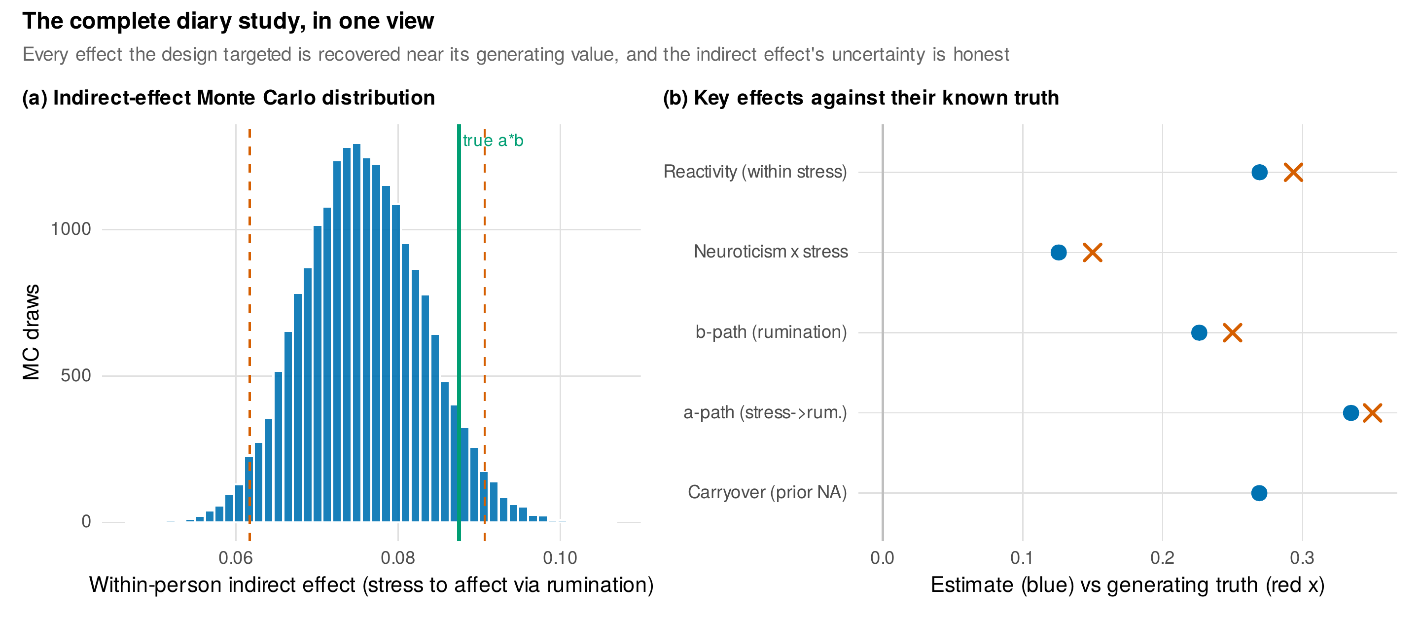
Note. (a) The Monte Carlo distribution of the within-person indirect effect (stress to affect via rumination), with its 95% interval and the true \(a\,b\). (b) The study’s key effects, estimated (blue) against their generating truth (red crosses); every effect the design targeted is recovered near its true value. The complete script is shipped as ch23_analysis_V01.R.
The results section that reports such a study has obligations beyond a table of coefficients, and Table 23.6 extends the reporting checklist of Chapter 13 with the intensive-longitudinal specifics: the centering statement, saying exactly which predictors were person-centered and how the person means were entered; the lag construction, saying how lags were formed and whether they crossed the overnight gap; the cycle and trend decisions, saying what was modeled and what was partialled; the dependence handling, saying whether AR(1) residuals or a lagged outcome was used and why; and the software and versions, because these models are sensitive to estimator and optimizer. Gabriel and colleagues (2019) and the open handbook of Myin-Germeys and Kuppens (2021) collect the field’s emerging standards, and Nezlek (2011) and Hoffman (2015) give book-length treatments of the modeling. The pitfalls, practice, and software boxes gather the recurring hazards, the convergence economics, and the syntax.
Common Pitfall • Four ways an intensive-longitudinal analysis goes wrong
First, centering a time-varying predictor on its full-sample person mean when the predictor trends, which lets the trend leak into the within-person effect; detrend first when a fluctuation question meets a trend. Second, constructing lags that silently cross the overnight gap, so that the first beep of a day is regressed on the last beep of the day before as though no night intervened; lag within days, or decide the night-gap treatment deliberately. Third, reading the covariate effects in a lagged-outcome model as total effects, when they are conditional on the prior state and answer a different question. Fourth, estimating a 1-1-1 mediation from two separate models and reporting \(a\,b\) as the indirect effect, forgetting the \(\mathrm{cov}(a_i,b_i)\) term that the random paths contribute.
In Practice • How many random slopes, and how much data
An intensive-longitudinal model can carry only so many random slopes before it fails to converge, and the Chapter 13.5 protocol applies: add random slopes for the effects whose heterogeneity is of interest, test them, and simplify the covariance structure before dropping the slopes themselves when convergence is difficult. Power in these designs has two sample sizes, the number of persons and the number of occasions per person, and they do different work: persons power the between-person questions and the moderators of within-person slopes, while occasions power the within-person effects and their heterogeneity. Detecting reactivity heterogeneity, a variance, is costly, needing both many people and many occasions each; the power tools of Chapter 4 quantify the trade-off, and the honest headline is that random-slope variances are harder to detect than fixed effects.
Software Note • intensive-longitudinal models across programs
In R, lme4 fits the two- and three-level random-slope models and lmerTest supplies the denominator degrees of freedom; nlme adds the AR(1) residual structure through correlation = corAR1(form = ~ occ | person), the route used here for serial dependence. The stacked 1-1-1 mediation is fitted in lme4 by stacking the mediator and outcome equations with selection indicators and letting the \(a\)- and \(b\)-path random effects covary; a Bayesian version in brms handles the random covariance and the indirect-effect interval together and is often cleaner when available. Mplus fits these as TYPE = TWOLEVEL models, and its dynamic structural equation modeling (DSEM) facility is the doorway to Chapter 25, where the lagged dynamics become the estimand rather than a nuisance. The complete analysis, every model and simulation in this chapter, is the shipped ch23_analysis_V01.R, with figures in ch23_figures_V01.R and the dataset built by gen_ema_stress_V01.R.
Table 23.6. Reporting checklist for intensive-longitudinal multilevel studies.
| Item | |
|---|---|
| 1 | Design: persons, days, beeps per day, sampling scheme, and compliance or missingness |
| 2 | Centering statement: which predictors were person-centered, and how person means were entered |
| 3 | Level structure: two-, three-level, or cross-classified, with the intraclass correlations justifying it |
| 4 | Cycle and trend decisions: what was modeled (diurnal, weekly, trend) and what was partialled as nuisance |
| 5 | Serial dependence: AR(1) residuals or lagged outcome, with the estimand each targets, and a residual ACF diagnostic |
| 6 | Random effects: which slopes were random, the covariance structure, and convergence |
| 7 | Mediation: the stacked or Bayesian estimator, the \(a\)-\(b\) covariance term, and the Monte Carlo or posterior interval |
| 8 | Software, estimator, optimizer, and versions |
Note. Extends the Chapter 13 checklist with the intensive-longitudinal specifics. The centering, lag-construction, cycle, trend, and dependence decisions are analytic choices that change the estimand, so each must be stated, not left implicit.
Chapter Summary
Intensive longitudinal designs make the within-person question askable, and the multilevel model answers it when its craft is respected. Person-mean centering isolates the within-person deviation from the between-person mean, and the within-person effect, its random slope, and the covariates that moderate that slope are the reactivity, its heterogeneity, and its explanation, the individual-differences findings that are the point of the enterprise. The nesting of moments in days in persons is read from the intraclass correlations, which decide between two-level, three-level, and cross-classified structures. Cycles, diurnal and weekly, are modeled with sine-cosine terms that reconstruct to an amplitude and phase and may vary across persons, and are partialled as nuisance or estimated as phenomenon by the question. Trends force a fork by estimand: a fluctuation question detrends, a change question models the trend, and centering without detrending lets a trend leak into the within-person effect. Serial dependence forks too: an AR(1) residual structure preserves the reactivity estimand and corrects its standard errors, while a lagged outcome makes carryover the estimand at the cost of a small-sample bias, upward with a random intercept and downward with fixed effects, that hands off to Chapter 25 when the dynamics are the target. Within-person 1-1-1 mediation adds the covariance of the random \(a\)- and \(b\)-paths to the product of their means, the term most often forgotten, and its uncertainty is a Monte Carlo or posterior interval. Reporting extends the multilevel checklist with the centering, lag, cycle, trend, and dependence decisions, because each is an analytic choice that changes what is being estimated.
Exercises
- 23.1 Specification grammar. For five “on occasions when” questions, write the multilevel formula and the centering plan, then trade critiques with a peer using Table 23.1 as the key.
- 23.2 Reactivity and moderation. On
ema_stress, fit the random-slope reactivity model, add the neuroticism cross-level interaction, probe it, and write the results paragraph. - 23.3 Cycle lab. Recover the diurnal amplitude and phase from the sine-cosine pair, add random trigonometric slopes, and interpret two people’s fitted rhythms.
- 23.4 Trend leak. Reproduce the leakage simulation of Figure 23.6, then write the decision memo explaining when to detrend and when to model the trend.
- 23.5 The lag fork. Fit both an AR(1) residual model and a lagged-outcome model to
ema_stress, and reconcile their estimands in words, naming what each coefficient means. - 23.6 Within-person mediation. Estimate the 1-1-1 mediation with a Monte Carlo interval, report the \(a\)-\(b\) covariance term, and state the random-effect caveats.
References
Bauer, D. J., Preacher, K. J., & Gil, K. M. (2006). Conceptualizing and testing random indirect effects and moderated mediation in multilevel models: New procedures and recommendations. Psychological Methods, 11(2), 142–163. https://doi.org/10.1037/1082-989X.11.2.142
Bolger, N., DeLongis, A., Kessler, R. C., & Schilling, E. A. (1989). Effects of daily stress on negative mood. Journal of Personality and Social Psychology, 57(5), 808–818. https://doi.org/10.1037/0022-3514.57.5.808
Bolger, N., & Laurenceau, J.-P. (2013). Intensive longitudinal methods: An introduction to diary and experience sampling research. Guilford Press.
Bolger, N., & Zuckerman, A. (1995). A framework for studying personality in the stress process. Journal of Personality and Social Psychology, 69(5), 890–902. https://doi.org/10.1037/0022-3514.69.5.890
Curran, P. J., & Bauer, D. J. (2011). The disaggregation of within-person and between-person effects in longitudinal models of change. Annual Review of Psychology, 62, 583–619. https://doi.org/10.1146/annurev.psych.093008.100356
Enders, C. K., & Tofighi, D. (2007). Centering predictor variables in cross-sectional multilevel models: A new look at an old issue. Psychological Methods, 12(2), 121–138. https://doi.org/10.1037/1082-989X.12.2.121
Gabriel, A. S., Podsakoff, N. P., Beal, D. J., Scott, B. A., Sonnentag, S., Trougakos, J. P., & Butts, M. M. (2019). Experience sampling methods: A discussion of critical trends and considerations for scholarly advancement. Organizational Research Methods, 22(4), 969–1006. https://doi.org/10.1177/1094428118802626
Hamaker, E. L., & Muthén, B. (2020). The fixed versus random effects debate and how it relates to centering in multilevel modeling. Psychological Methods, 25(3), 365–379. https://doi.org/10.1037/met0000239
Hektner, J. M., Schmidt, J. A., & Csikszentmihalyi, M. (2007). Experience sampling method: Measuring the quality of everyday life. SAGE Publications. https://doi.org/10.4135/9781412984201
Hoffman, L. (2015). Longitudinal analysis: Modeling within-person fluctuation and change. Routledge. https://doi.org/10.4324/9781315744094
Hoffman, L., & Stawski, R. S. (2009). Persons as contexts: Evaluating between-person and within-person effects in longitudinal analysis. Research in Human Development, 6(2–3), 97–120. https://doi.org/10.1080/15427600902911189
Laurenceau, J.-P., Barrett, L. F., & Pietromonaco, P. R. (1998). Intimacy as an interpersonal process: The importance of self-disclosure, partner disclosure, and perceived partner responsiveness in interpersonal exchanges. Journal of Personality and Social Psychology, 74(5), 1238–1251. https://doi.org/10.1037/0022-3514.74.5.1238
Liu, Y., & West, S. G. (2016). Weekly cycles in daily report data: An overlooked issue. Journal of Personality, 84(5), 560–579. https://doi.org/10.1111/jopy.12182
McNeish, D., & Stapleton, L. M. (2016). Modeling clustered data with very few clusters. Multivariate Behavioral Research, 51(4), 495–518. https://doi.org/10.1080/00273171.2016.1167008
Myin-Germeys, I., & Kuppens, P. (Eds.). (2021). The open handbook of experience sampling methodology: A step-by-step guide to designing, conducting, and analyzing ESM studies (2nd ed.). Center for Research on Experience Sampling and Ambulatory Methods Leuven.
Nezlek, J. B. (2011). Multilevel modeling for social and personality psychology. SAGE Publications. https://doi.org/10.4135/9781446287996
Nickell, S. (1981). Biases in dynamic models with fixed effects. Econometrica, 49(6), 1417–1426. https://doi.org/10.2307/1911408
Preacher, K. J., Zyphur, M. J., & Zhang, Z. (2010). A general multilevel SEM framework for assessing multilevel mediation. Psychological Methods, 15(3), 209–233. https://doi.org/10.1037/a0020141
Vuorre, M., & Bolger, N. (2018). Within-subject mediation analysis for experimental data in cognitive psychology and neuroscience. Behavior Research Methods, 50(5), 2125–2143. https://doi.org/10.3758/s13428-017-0980-9
Wang, L. P., & Maxwell, S. E. (2015). On disaggregating between-person and within-person effects with longitudinal data using multilevel models. Psychological Methods, 20(1), 63–83. https://doi.org/10.1037/met0000030
West, S. G., & Hepworth, J. T. (1991). Statistical issues in the study of temporal data: Daily experiences. Journal of Personality, 59(3), 609–662. https://doi.org/10.1111/j.1467-6494.1991.tb00261.x