Chapter 24
Time Series Analysis for Single Subjects
The previous chapter used many measurements from many people and asked, at bottom, a within-person question answered by pooling across persons. This chapter narrows the lens to one person and refuses to pool. When a single individual is measured densely over time, a clinical patient monitored daily, a personality researcher’s single case, a participant sampled many times a day for weeks, the series that results is a legitimate object of analysis in its own right, and the tools that analyze it are the classical time series methods of the physical and economic sciences, imported into psychology and bent to fit its data. That import is the subject of the chapter. Psychological series are short where econometric series are long, noisy where they are clean, missing where they are complete, and bounded where they are free, and every classical assumption strains against those facts. The chapter teaches the core apparatus honestly: weak stationarity as the load-bearing precondition, the autocorrelation and partial-autocorrelation functions as process signatures, the autoregressive coefficient as psychological carryover rather than a nuisance to be swept away, the interrupted time series as the design that makes a single person their own control, and P-technique factor analysis as the historical root of the idiographic program that Chapters 25 through 28 carry forward. It closes on the question every reader with an intensive dataset must face and few ask out loud, which is how long a series has to be before any of this is trustworthy.
Learning Objectives
After working through this chapter, you should be able to: (1) define weak stationarity and diagnose its violations, trend, cycles, and variance shifts, both visually through rolling statistics and through the ADF and KPSS tests, while recognizing the low power of those tests at psychological series lengths; (2) read the autocorrelation and partial-autocorrelation functions as signatures that identify candidate autoregressive-moving-average structures; (3) fit and check AR, MA, and ARMA models, judge residual whiteness with the Ljung-Box test at the correct degrees of freedom, and interpret the parameters psychologically as inertia and, through complex roots, as oscillation; (4) distinguish differencing from detrending and state which psychological question each answers; (5) analyze an interrupted time series for single-case intervention evaluation, estimating level and slope change with autocorrelated errors and confronting the small-sample inference problem honestly; (6) run a P-technique factor analysis, articulate its insight into person-specific structure and its serial-dependence flaw, and locate the repair in the dynamic factor models of Chapter 26; and (7) state what series length these methods require and report a single-subject analysis credibly.
24.1 Why Study One Person Seriously
The idiographic claim, introduced in Chapter 1 and now given teeth, is that a single person measured repeatedly is not an underpowered sample of one but a population in time, and that the structure of that person’s process is a scientific target that no amount of between-person data can reach. Three research programs make the claim concrete. Clinical monitoring tracks one patient’s symptoms across days or weeks to detect deterioration, evaluate a treatment, and tailor care, a use with a long history in single-case experimental design and a growing one in the digital-phenotyping present (Borckardt et al., 2008). Personality and emotion research studies the person as a dynamic system whose regulatory tendencies, how fast affect returns to baseline, whether it overshoots and swings back, are individual-differences constructs measured only within the person over time (Suls et al., 1998; Kuppens et al., 2010). And theory-testing in the idiographic tradition treats generalization as a matter of systematic replication across persons rather than aggregation over them, so that a finding earns its status by recurring in one individual after another, the same logic that Chapter 25 will recast as the random effects of a multilevel model, a meta-analysis of persons conducted inside a single fitted object.
The reason this matters, and the reason the idiographic program is more than a methodological preference, is that between-person structure and within-person structure need not agree. A factor model estimated across people describes how individuals differ from one another; a factor model estimated within one person across occasions describes how that person’s states move together over time; and the ergodic theorems make precise that the two coincide only under conditions, stationarity and homogeneity across the population, that psychological processes routinely violate (Molenaar, 2004; Molenaar & Campbell, 2009). When they fail, the group-level structure is not a summary of the individuals but a separate object, and inferences from one level to the other are unwarranted. The empirical demonstration that the two levels genuinely differ, that group-to-individual generalizability cannot be assumed, is the manifesto’s cash value (Fisher et al., 2018; Beltz et al., 2016), and it is the intellectual charter for analyzing the single person on the person’s own terms.
Before the classical machinery is imported, its assumptions must be weighed against the data psychology actually produces. Figure 24.1 sets a psychological series beside an econometric one. The econometric series is long, often hundreds or thousands of equally spaced observations, measured with instruments of high reliability and few gaps. The psychological series is short, fifty to a few hundred occasions in a typical intensive study, noisy, punctuated by missed beeps and skipped days, measured on bounded scales that floor and ceiling, and reactive, in that the act of measurement can change the thing measured. The classical tools transfer, but their large-sample justifications strain at psychological length, their stationarity assumptions strain against developmental drift, and their complete-data derivations strain against missingness. The chapter’s recurring discipline is to use each tool while stating exactly where the transfer weakens.
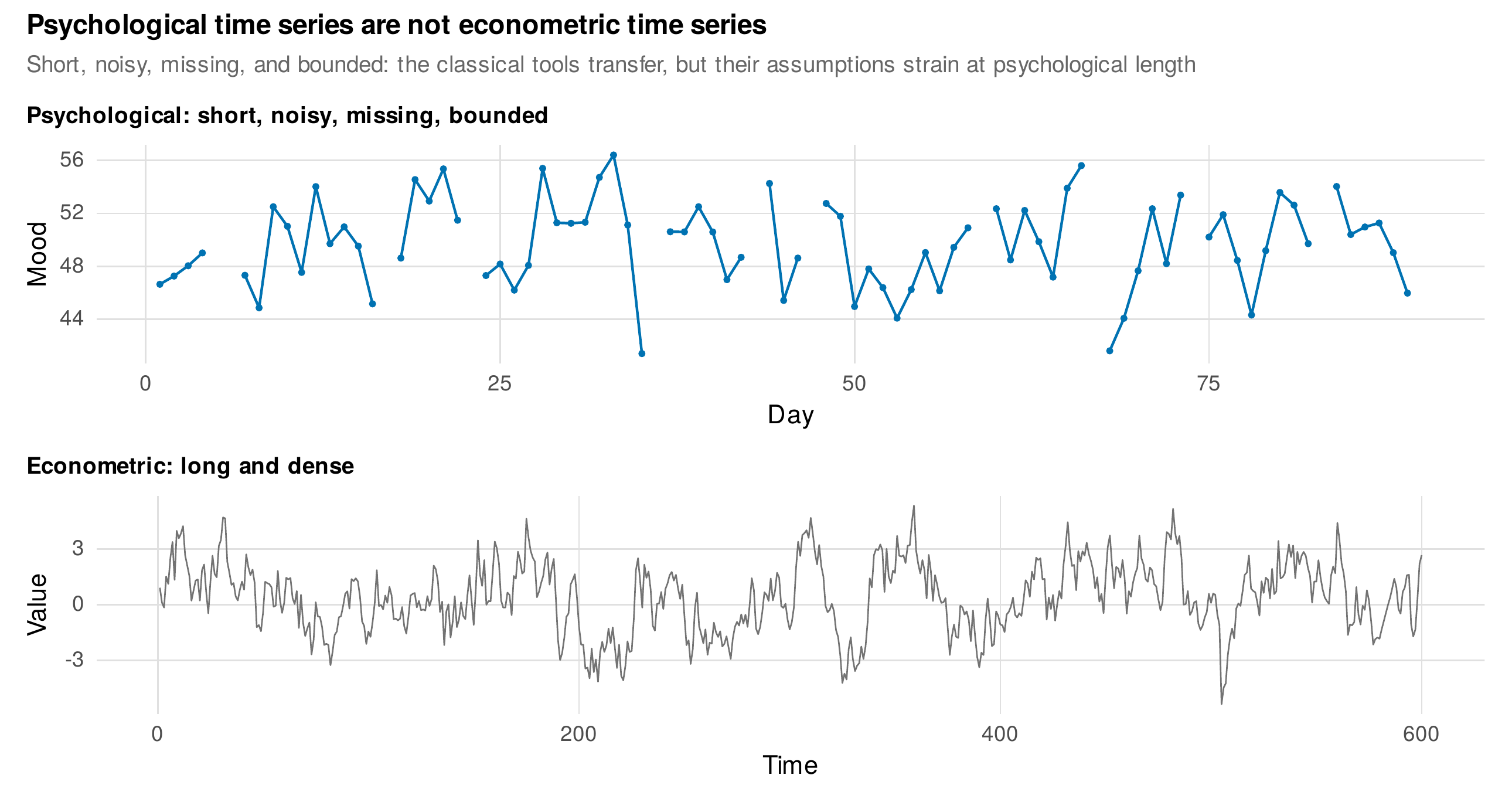
Note. Top: ninety days of one person’s negative mood, short, noisy, bounded, and with missed days shown as gaps. Bottom: a long, clean, densely sampled series of the kind classical time series methods were built for. The methods of this chapter were derived for the lower series and are applied here to the upper one; their assumptions transfer only with care.
The worked series for the chapter is mood_ts, one hundred eighty daily reports of negative mood from a single person on a zero to one hundred scale. The data-generating process is known, because the series is simulated to carry exactly the phenomena the chapter teaches: a stationary second-order autoregression with complex roots forms the baseline, so that the person’s mood carries itself forward and gently oscillates; an intervention is planted on day ninety-one as an immediate level drop and a subsequent change in slope; and a late shift in innovation variance is planted on day one hundred fifty-one, a nonstationarity of a kind deferred to Chapter 32 and used here only as something the stationarity diagnostics must catch. Knowing the truth lets every estimate be checked against the value that produced it, which is the standard the book holds itself to throughout.
24.2 Stationarity: The Load-Bearing Concept
Nearly everything that follows presupposes weak stationarity, and so the concept is worth stating precisely before it is used. A series is weakly, or covariance, stationary when three conditions hold: its mean does not depend on time, its variance does not depend on time, and its autocovariance between two occasions depends only on the lag between them and not on where in the series they fall. The reason stationarity is load-bearing rather than a technicality is that the entire vocabulary of dynamics, the autoregressive coefficient, the autocorrelation function, the notion of a shock decaying, is defined by quantities that are assumed constant over the series. If the mean wanders, a regression of the series on its own past will confound the wandering with the carryover and report an inertia that is really a trend; if the variance shifts, a single autoregressive coefficient will average two regimes that ought to be described separately. Estimating dynamics on a nonstationary series does not merely lose efficiency, it estimates a parameter that does not exist.
Diagnosis begins with the eye, not the test. The rolling mean and the rolling standard deviation, computed in a moving window and displayed against the series, reveal a wandering level or a changing spread more reliably at psychological length than any formal procedure. Figure 24.2 is a gallery of the four cases the analyst must learn to distinguish by sight: a stationary series whose rolling mean and spread are flat; a trended series whose rolling mean climbs; a variance-shifting series whose rolling mean holds but whose rolling spread widens; and a regime-switching series whose level jumps partway through. Each demands a different response, and the response depends on the estimand, a point developed below.
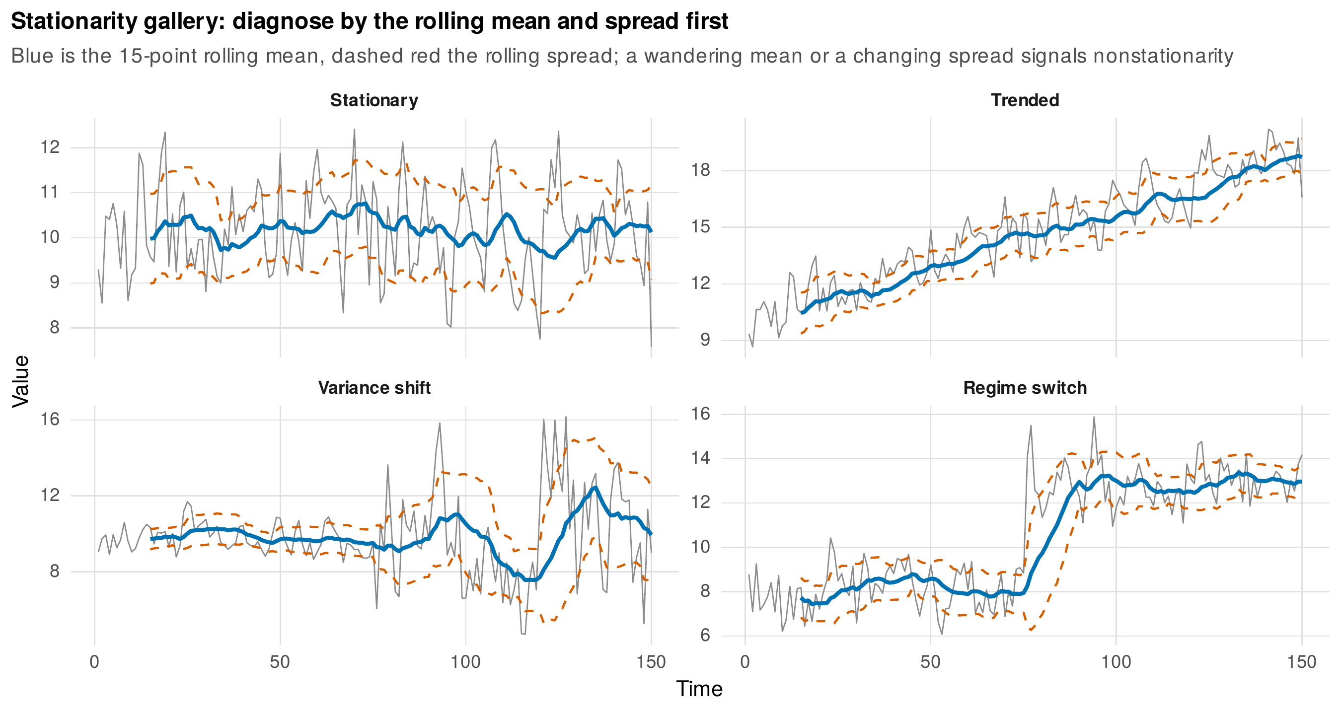
Note. Each panel shows a series (grey) with its fifteen-point rolling mean (blue) and rolling spread (dashed red band). A flat rolling mean and spread indicate stationarity; a climbing mean indicates a trend; a widening band indicates a variance shift; a jump in the mean indicates a regime switch. Visual diagnosis precedes formal testing.
The formal tests come second and are best used as a pair, because the two standard tests carry opposite null hypotheses. The augmented Dickey-Fuller (ADF) test takes nonstationarity, a unit root, as its null and rejects in favor of stationarity; the KPSS test takes stationarity as its null and rejects in favor of nonstationarity. Run together, they can corroborate, when ADF rejects and KPSS does not, both point to stationarity, or they can conflict, when neither rejects, a common outcome at short length that signals only that the data are uninformative about the question. On the baseline segment of mood_ts, the ADF statistic is \(-7.02\) against a five-percent critical value of \(-2.88\), decisively rejecting a unit root, and the KPSS statistic is \(0.050\) against a five-percent critical value of \(0.463\), nowhere near rejecting stationarity. The two tests agree, and the agreement is trustworthy here because the baseline was generated as a stationary process. The agreement should not be expected to be so clean in real data of the same length.
The honesty the section owes the reader concerns power. The unit-root tests were designed for economic series of several hundred to several thousand observations, and at psychological length they are badly underpowered, meaning they frequently fail to reject a unit root even when the series is stationary. A small simulation makes the failure numerical. Generating stationary AR(1) series with a moderate autoregressive coefficient and applying the ADF test, the probability of correctly rejecting the unit root is only \(0.47\) at \(T=30\), rises to \(0.88\) at \(T=50\), and reaches near certainty only by \(T=100\). At the lengths of many diary studies, then, a non-rejection by the ADF test is nearly uninformative, and the visual diagnosis carries most of the evidential weight. This is the first of several places where the chapter’s numbers, produced by simulation rather than asserted, tell the reader something the textbooks state only qualitatively.
Sources of nonstationarity in psychological data map to remedies, and the remedy is dictated by the estimand rather than chosen for statistical convenience, as Table 24.1 sets out. A linear or curvilinear trend, mood improving over a semester, arises when a slow developmental process rides underneath the fluctuations. If the fluctuations are the target, the trend is removed by detrending, regressing the series on time and analyzing the residuals, which preserves the fluctuation dynamics on the original scale. If the change itself is the target, the trend is modeled, not removed. A slow cycle, a weekly rhythm in a daily series, is nonstationary within a short window but is handled by modeling the cycle with the sine and cosine terms of Chapter 23 rather than by differencing. A variance shift or a regime change signals that the series is generated by more than one process, and the appropriate response is to model the change point explicitly, the subject of Chapter 32, rather than to force a single stationary model across the break. Differencing, replacing each value by its change from the previous occasion, is the econometric reflex for a trend, but it exacts a psychological cost that the next section spells out and should be used sparingly and with a stated reason.
Table 24.1. Nonstationarity: violation, diagnosis, remedy, and estimand consequence.
| Violation | Diagnosis | Remedy | Estimand consequence |
|---|---|---|---|
| Linear or curvilinear trend | Rolling mean climbs or bends; ACF decays very slowly | Detrend if fluctuation is the target; model the trend if change is the target | Detrending keeps the fluctuation estimand; differencing changes it to change-score dynamics |
| Slow cycle (weekly, diurnal) | Periodic rolling mean; ACF peaks at the period | Model with sine-cosine terms (Chapter 23) | The cycle becomes a modeled component, not a contaminant of the AR estimate |
| Variance shift | Rolling spread widens or narrows; level roughly constant | Model the change point (Chapter 32); segment the series | A single AR variance averages two regimes and describes neither |
| Regime switch (level jump) | Rolling mean steps; two plateaus | Change-point or intervention model (Section 24.4; Chapter 32) | One stationary model across the break estimates a nonexistent common process |
| Unit root (stochastic trend) | ADF fails to reject; KPSS rejects; ACF near one at all lags | Difference once, having ruled out the alternatives above | Differencing answers a change-dynamics question, not a level-dynamics one |
Note. The remedy is chosen by the estimand, not by a test. Detrending and differencing both remove a trend but leave different series behind and answer different questions. ADF and KPSS carry opposite nulls and are read jointly.
Foundations Box • The AR(1) half-life and the AR(2) stationarity triangle
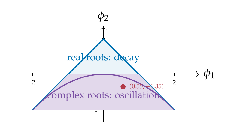
For a stationary first-order autoregression \(x_t = \phi\, x_{t-1} + \varepsilon_t\) with \(|\phi|<1\), the process has mean zero, variance \(\sigma^2_\varepsilon/(1-\phi^2)\), and autocorrelation \(\rho_k = \phi^{k}\) at lag \(k\), so the autocorrelation decays geometrically. A one-unit shock at time \(t\) contributes \(\phi^{k}\) to the series \(k\) steps later, and the number of steps for that contribution to fall to half its size, the half-life of a perturbation, is \(h = \ln(0.5)/\ln|\phi|\). The half-life turns an abstract coefficient into a sentence a clinician can use: at \(\phi=0.5\) a shock is half gone in one step, at \(\phi=0.8\) in about three, at \(\phi=0.95\) in about fourteen. For the second-order process \(x_t = \phi_1 x_{t-1} + \phi_2 x_{t-2} + \varepsilon_t\), stationarity requires the coefficient pair to lie inside a triangle: \(\phi_1+\phi_2<1\), \(\phi_2-\phi_1<1\), and \(\phi_2>-1\). Inside that triangle, the region below the parabola \(\phi_2 = -\phi_1^2/4\) produces complex roots and therefore a damped oscillation rather than a smooth decay, which is the algebraic source of the overshoot-and-return that emotion-dynamics researchers read as regulation. The point below marks the truth of the worked series, which lies in the oscillation region.
24.3 The ARMA Toolkit
The autoregression of order one is the psychological workhorse of this chapter, and its coefficient is the chapter’s central quantity, so it is worth insisting on the interpretation before the algebra accumulates. In \(x_t = \phi\, x_{t-1} + \varepsilon_t\), the coefficient \(\phi\) is inertia, the degree to which the person’s present state is carried over from the immediately preceding one, and the emotion-dynamics literature reads it as the sluggishness of affective regulation, the tendency of a mood to persist rather than return quickly to baseline (Suls et al., 1998; Kuppens et al., 2010). The half-life derived in the foundations box turns the coefficient into a clinical statement about how long a disturbance lingers. Figure 24.3 shows three simulated series at \(\phi\) equal to zero, four-tenths, and eight-tenths, with the half-lives annotated, and the visual lesson is immediate: at zero the series is white noise with no memory, at four-tenths a shock is half gone within a step, and at eight-tenths disturbances pile into slow, persistent swings. The autocorrelation is not a nuisance to be corrected away, as the older methodological literature treated it; here it is the finding.
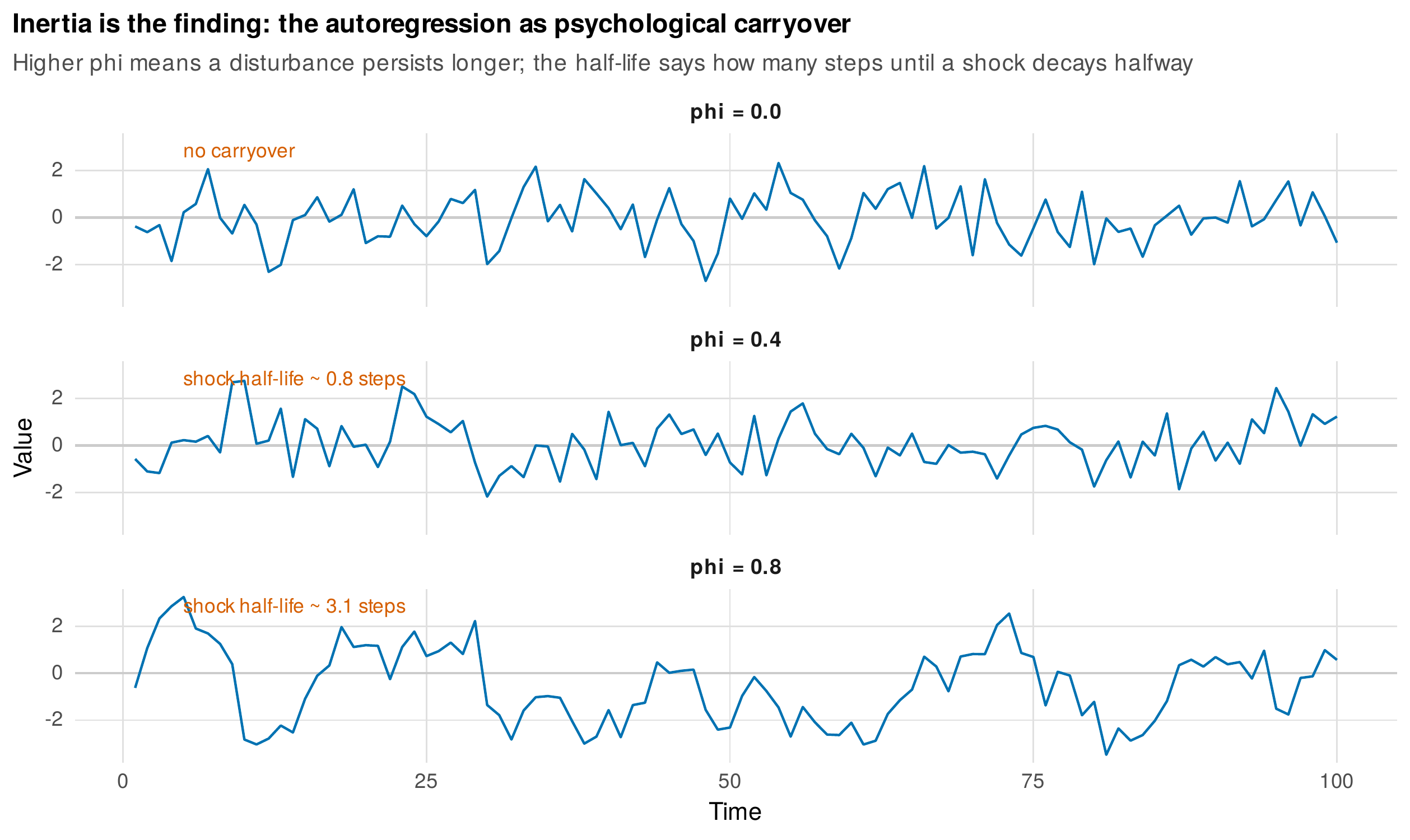
Note. Three AR(1) series at \(\phi=0\), \(0.4\), and \(0.8\). Higher \(\phi\) makes disturbances persist, visible as slower, more sustained swings, and the annotated half-life gives the number of steps for a shock to decay halfway. The autoregressive coefficient is a substantive individual difference, not a statistical nuisance.
Extending to order two admits a qualitatively new behavior. In \(x_t = \phi_1 x_{t-1} + \phi_2 x_{t-2} + \varepsilon_t\), a negative second-order coefficient of sufficient magnitude gives the characteristic polynomial complex roots, and complex roots make the autocovariance oscillate: the series overshoots its mean, swings back, overshoots the other way, and settles, a damped rhythm rather than a smooth return. The worked series was built with \(\phi_1=0.55\) and \(\phi_2=-0.35\), a pair inside the stationarity triangle and below the complex-root parabola, giving a damped oscillation with a period near \(5.8\) days. Figure 24.4 shows a realization, and the psychological reading is the emotion-dynamics one: a person whose affect not only carries forward but tends to correct past itself, the signature of a regulatory system that overshoots. Chapter 32 gives this oscillation an explicit differential-equation form as a damped linear oscillator; here it is the second-order autoregression’s most psychologically interesting face.
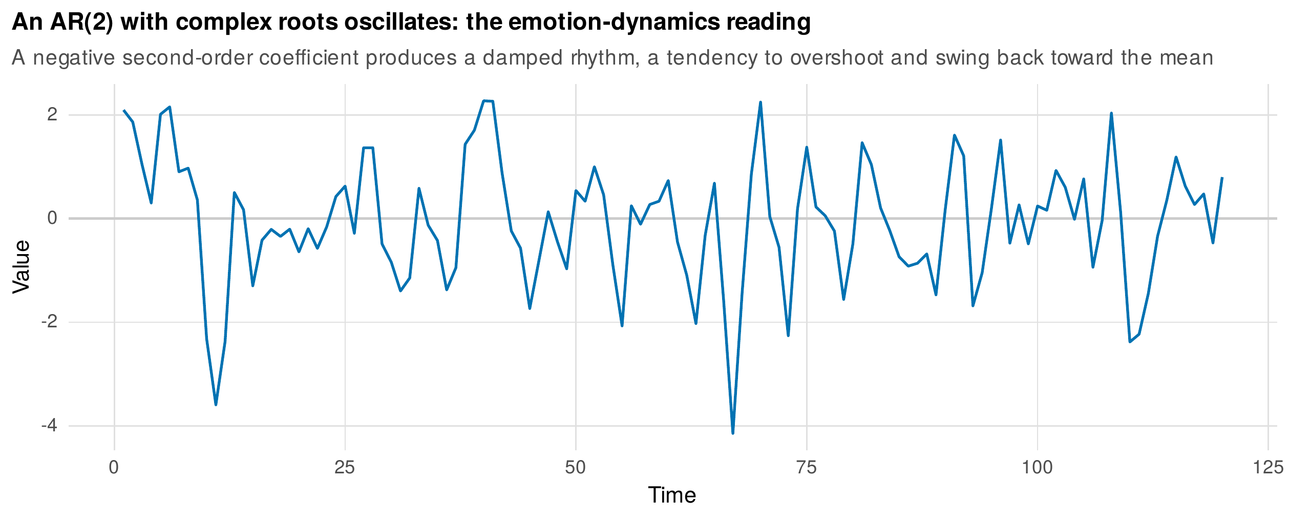
Note. A second-order autoregression with \(\phi_1=0.55\), \(\phi_2=-0.35\). The negative second-order coefficient yields complex roots and a damped oscillation with a period near six occasions, a tendency to overshoot the mean and swing back that emotion researchers interpret as a regulatory dynamic.
Moving-average processes describe a complementary form of memory. In \(x_t = \varepsilon_t + \theta\, \varepsilon_{t-1}\), the present depends not on the past state but on the past shock, so that a disturbance persists for a fixed number of occasions and then vanishes cleanly, in contrast to the autoregression’s geometric fade. The mixed ARMA process combines the two, and for most psychological purposes a low-order AR or ARMA suffices. The classical strategy for choosing the order, the Box-Jenkins method, reads the autocorrelation and partial-autocorrelation functions as signatures (Box et al., 2015). The autoregression of order \(p\) has a partial autocorrelation that cuts off sharply after lag \(p\) while its autocorrelation decays; the moving average of order \(q\) has an autocorrelation that cuts off after lag \(q\) while its partial autocorrelation decays; the mixed process has both functions tailing off. Figure 24.5 displays the four canonical signatures, and Table 24.2 states the identification rules that generate them.
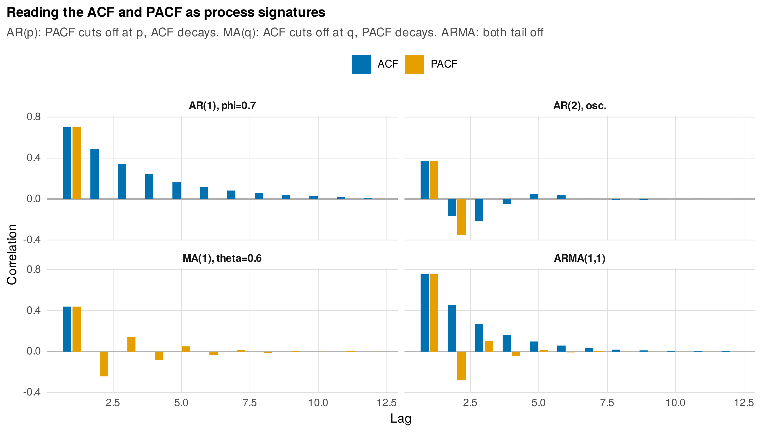
Note. Theoretical autocorrelation (blue) and partial autocorrelation (orange) for four processes. AR(\(p\)): the partial autocorrelation cuts off after lag \(p\), the autocorrelation decays. MA(\(q\)): the autocorrelation cuts off after lag \(q\), the partial autocorrelation decays. ARMA: both tail off. These signatures are the Box-Jenkins identification heuristic in visual form.
Table 24.2. ACF and PACF identification signatures.
| Process | Autocorrelation (ACF) | Partial autocorrelation (PACF) | Reading |
|---|---|---|---|
| AR(\(p\)) | Decays (geometric or damped-sine) | Cuts off after lag \(p\) | Order \(p\) from the PACF cutoff |
| MA(\(q\)) | Cuts off after lag \(q\) | Decays | Order \(q\) from the ACF cutoff |
| ARMA(\(p,q\)) | Tails off after lag \(q\) | Tails off after lag \(p\) | Neither cuts off; use information criteria |
| White noise | All lags near zero | All lags near zero | No serial structure |
| Nonstationary | Decays very slowly, near one | Large spike at lag one | Difference or detrend first |
Note. The cutoff-versus-decay contrast is the heuristic core of Box-Jenkins identification. At short series length the sampling variability of these functions is large, and the visual signature should be corroborated by information-criterion comparison rather than trusted alone.
Identification by eye is a heuristic, not a proof, and at psychological length it is fragile because the sampling variability of the sample autocorrelations is large enough to blur the cutoff-versus-decay distinction. The modern complement is information-criterion selection, fitting a small set of candidate orders and comparing them by the AIC or BIC, with the caveat that at short length these criteria will happily overfit, selecting spurious moving-average terms that will not replicate. The worked fit illustrates both the promise and the caution. On the ninety-day baseline segment of mood_ts, the sample partial autocorrelation shows a spike at lag one of \(0.31\) and a second at lag two of \(-0.24\) before falling into the noise band, the AR(2) signature, and the information criteria agree, with the AR(2) model achieving the lowest AIC (\(458.2\)) and the lowest BIC (\(468.2\)) against the AR(1) (\(461.7\), \(469.2\)) and the ARMA(1,1) (\(460.1\), \(470.1\)). The fitted coefficients are \(0.38\) and \(-0.24\), attenuated from the generating \(0.55\) and \(-0.35\) but of the right sign and magnitude, the attenuation being the expected cost of estimating a second-order structure from only ninety observations, and the implied oscillation period of \(5.4\) days recovers the planted \(5.8\). This attenuation is not a coding error but the honest behavior of the estimator at psychological length, and it foreshadows Section 24.6.
Estimation and checking complete the arc. The parameters may be fitted by conditional or full maximum likelihood, which differ negligibly at these lengths, and the fitted model is judged by whether it has whitened the series, whether the residuals retain any serial structure. The Ljung-Box portmanteau test pools the residual autocorrelations into a single statistic, and the crucial subtlety, the one most often botched in applied work, is that its degrees of freedom must be reduced by the number of autoregressive and moving-average parameters estimated, because those parameters have already absorbed some of the autocorrelation. For the AR(2) fit, the Ljung-Box test on the residuals returns \(p=0.93\) at the corrected degrees of freedom, no evidence of remaining structure, and the model is retained. Had the degrees of freedom not been corrected, the test would have been anticonservative, too ready to declare the residuals white. The run-it-in-R panel below walks the full arc on the baseline segment, from stationarity check to identification to fit to residual diagnosis.
# The Box-Jenkins arc on one person's baseline mood series
d <- readRDS("Examples/data/mood_ts.rds")
base <- d$y[d$phase == "baseline"]        # T = 90 daily reports

# 1. Stationarity: eye first, then the paired tests
plot.ts(base)                              # rolling mean/spread by eye
adf_test(base); kpss_test(base)            # ADF rejects unit root; KPSS does not

# 2. Identification: ACF and PACF as signatures
acf(base, lag.max = 15); pacf(base, lag.max = 15)   # PACF cuts off at lag 2

# 3. Selection: compare candidate orders by information criterion
fit1 <- arima(base, order = c(1,0,0))      # AR(1)
fit2 <- arima(base, order = c(2,0,0))      # AR(2): lowest AIC and BIC
fitm <- arima(base, order = c(1,0,1))      # ARMA(1,1)
AIC(fit1, fit2, fitm); BIC(fit1, fit2, fitm)

# 4. Interpretation: phi as inertia, complex roots as oscillation
coef(fit2)                                 # ar1 ~ 0.38, ar2 ~ -0.24
# period of the damped oscillation, in days:
2*pi / acos( coef(fit2)[1] / (2*sqrt(-coef(fit2)[2])) )   # ~ 5.4

# 5. Checking: residual whiteness with corrected degrees of freedom
Box.test(residuals(fit2), lag = 10, type = "Ljung-Box", fitdf = 2)   # p = 0.93
Two further matters complete the toolkit: the choice between differencing and detrending, and the handling of missing occasions. When a trend is present, the analyst may remove it by differencing, analyzing the change from occasion to occasion, or by detrending, regressing on time and analyzing the residual fluctuation, and the two are not interchangeable because they answer different questions and leave different series behind. Figure 24.6 takes a single trended series through both routes and shows their autocorrelation functions. The raw series has an autocorrelation near \(0.95\) at lag one, the artifact of the trend; detrending returns a lag-one autocorrelation of \(0.31\), the genuine fluctuation dynamics; differencing returns \(-0.37\), a negative autocorrelation that is the signature of overdifferencing, of having converted a level process into a change process and thereby changed the question from how the person’s mood fluctuates to how the person’s day-to-day changes relate. For a psychological fluctuation question, detrending is almost always the right route, and differencing should be reserved for series with a genuine stochastic trend and justified out loud.
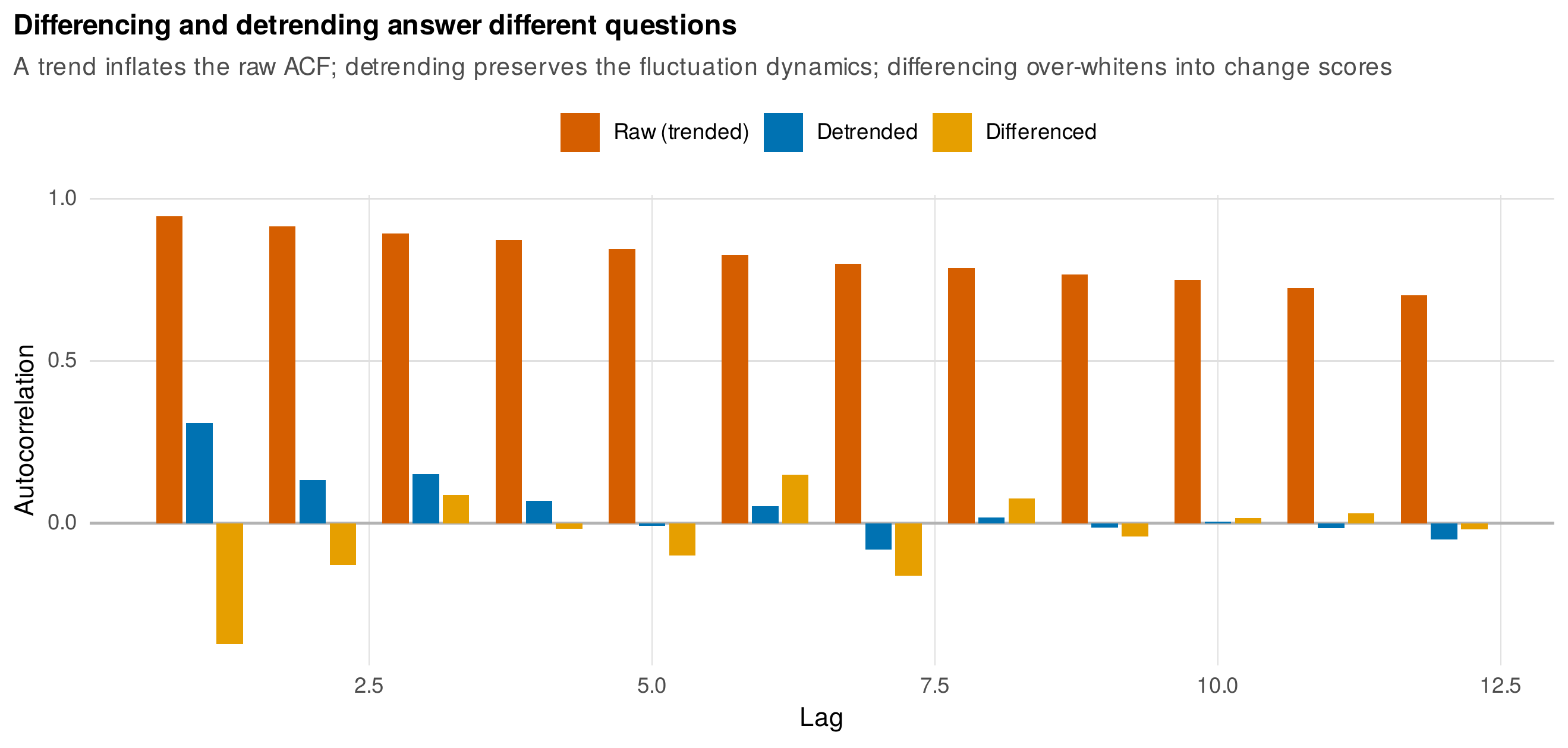
Note. Lag-wise autocorrelation of the same trended series left raw (red), detrended (blue), and differenced (orange). The trend inflates the raw autocorrelation toward one; detrending recovers the fluctuation dynamics; differencing over-whitens into a negative lag-one autocorrelation, the mark of a change-score series answering a different question.
Missing occasions are endemic in psychological series and are the point at which naive practice does the most quiet damage. The tempting fix, filling each gap by linear interpolation between its neighbors, manufactures autocorrelation, because an interpolated value is by construction a smooth blend of its surroundings and therefore more similar to them than a real observation would be. Figure 24.7 demonstrates the inflation on the worked series: the lag-one autocorrelation of the complete series is \(0.42\), and after deleting a fraction of occasions and filling them by interpolation it rises to \(0.57\), a spurious increase in apparent inertia of a third. The methodologically correct treatment, which does not distort the dynamics, is to keep the gaps and let a state-space model handle them through the Kalman filter, the subject of Chapter 26, or at minimum to fit the model on the observed occasions with a likelihood that respects the missingness rather than inventing data to fill it.
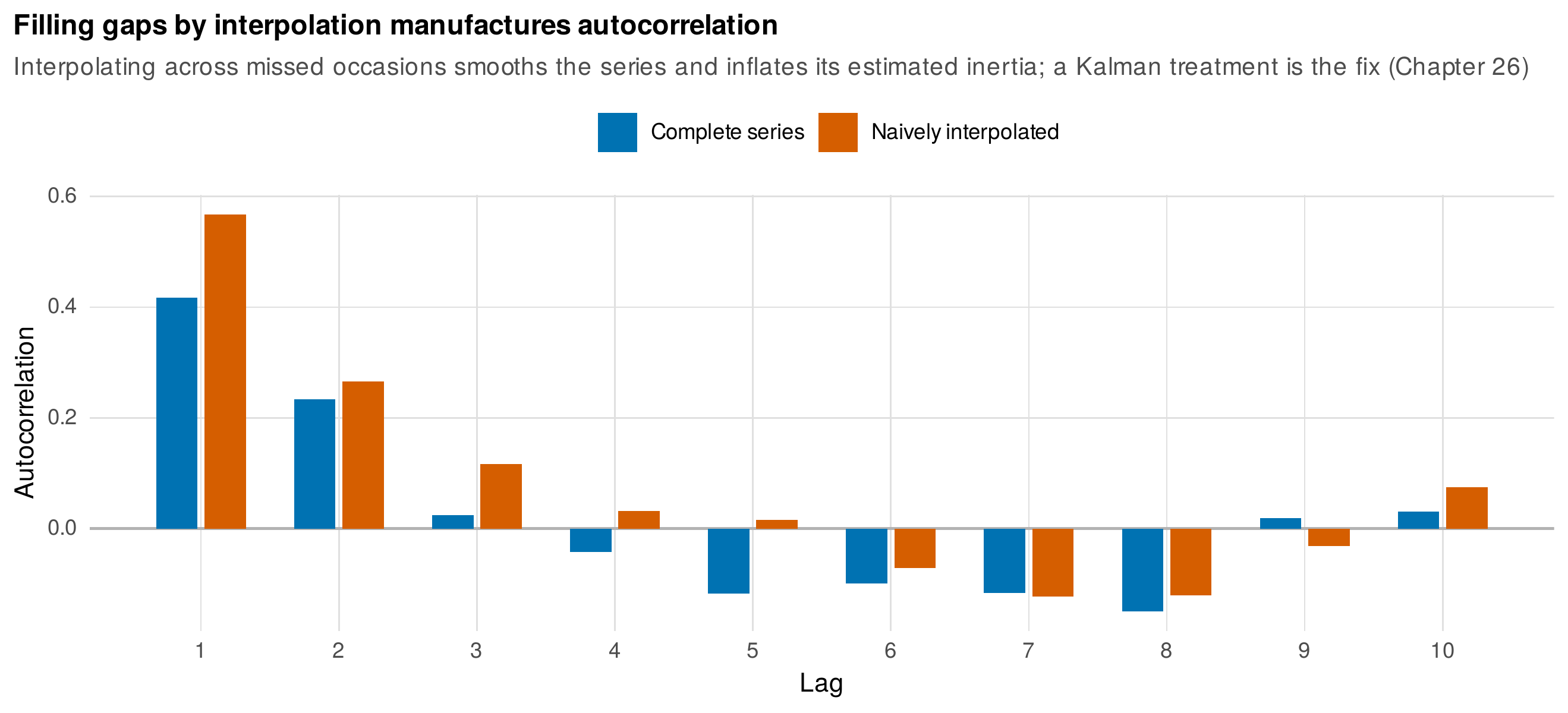
Note. Lag-wise autocorrelation of the complete series (blue) and of the same series after deleting occasions and filling them by linear interpolation (red). Interpolation smooths the series and inflates its estimated inertia, here raising the lag-one autocorrelation from \(0.42\) to \(0.57\). A Kalman treatment (Chapter 26) is the correct alternative.
Table 24.3 collects the parameters of the ARMA family with the psychological semantics that this chapter insists each one carries, because a coefficient reported without its meaning is a number a reviewer cannot evaluate and a clinician cannot use.
Table 24.3. ARMA parameter interpretation glossary.
| Parameter | Statistical meaning | Psychological semantics |
|---|---|---|
| \(\phi_1\) (AR1) | Lag-one autoregression | Inertia or carryover: how much of the present state persists from the last occasion; half-life \(\ln(0.5)/\ln|\phi_1|\) |
| \(\phi_2\) (AR2) | Lag-two autoregression | With \(\phi_1\), sets whether the process decays smoothly or oscillates; a negative \(\phi_2\) below the parabola gives regulatory overshoot |
| \(\theta\) (MA1) | Lag-one moving average | Shock persistence: how long a one-time disturbance is felt before it clears, independent of the state’s own memory |
| \(\sigma^2_\varepsilon\) | Innovation variance | Moment-to-moment lability: the size of the unpredictable disturbances entering the system |
| Complex roots | Roots of the AR polynomial off the real line | Damped oscillation: overshoot-and-return; period \(2\pi/\arccos(\phi_1/2\sqrt{-\phi_2})\) |
| Half-life | \(\ln(0.5)/\ln|\phi|\) | Occasions until a perturbation decays halfway; the clinician’s translation of inertia |
Note. Every parameter is reported with its psychological reading. The autoregressive coefficients are individual-differences constructs, not nuisance corrections; the innovation variance is lability; complex roots are regulatory oscillation.
Software Note • The R time-series ecosystem and an arima() naming trap
The base stats package supplies arima(), acf(), pacf(), ar(), and Box.test(), which cover everything in this chapter. Two ecosystems extend them. The older forecast package (Hyndman) provides auto.arima() for automatic order selection and a mature forecasting apparatus; the newer fable package, part of the tidyverts, reimplements the same modeling in a tidy, tibble-based interface and is the direction the ecosystem is moving, though forecast remains widely used and fully supported. For a single short series either is more machinery than the task needs; base arima() with a hand comparison of a few orders is transparent and sufficient. One naming trap deserves flagging: the intercept that arima() reports is not a regression intercept but the estimated process mean, printed under the label intercept in the coefficient vector. Reading it as the constant of the autoregressive equation, which would be the mean times \((1-\sum\phi)\), is a common and consequential error. When automatic selection is used, verify that the chosen order is stable across a reasonable sample and not an artifact of overfitting at short length.
24.4 Interrupted Time Series for Single-Case Research
The interrupted time series is the design that turns a single person’s series into a controlled comparison. Its logic is that the person serves as their own control: a baseline phase establishes the trajectory the person would have continued along, an intervention is introduced at a known point, and the change in the trajectory after that point, against the counterfactual of no intervention, is the treatment effect. The design has real threats, chief among them history, some other event coinciding with the intervention, and maturation, a trend that would have occurred anyway, and these are the reasons the baseline phase must be long enough to establish the counterfactual trajectory credibly and the reason multiple-baseline designs, staggering the intervention across behaviors or settings, strengthen the inference by making a coincident history implausible (McCleary et al., 2017; Kratochwill et al., 2010).
The statistical model is a segmented regression. Writing \(y_t\) for the outcome, \(t\) for time, and \(D_t\) for an indicator that switches from zero to one at the intervention, the model \(y_t = \beta_0 + \beta_1 t + \beta_2 D_t + \beta_3 (t - t^\ast) D_t + e_t\) estimates a baseline level \(\beta_0\), a baseline slope \(\beta_1\), an immediate level change \(\beta_2\) at the intervention, and a change in slope \(\beta_3\) thereafter. The level change is the discontinuous jump at the moment of intervention; the slope change is the difference in trajectory that accumulates afterward; and the two together decompose the intervention’s effect into an immediate shift and a change in trend. Figure 24.8 shows the anatomy on mood_ts, whose intervention was planted on day ninety-one as a level drop of six points and a slope change of five-hundredths of a point per day.
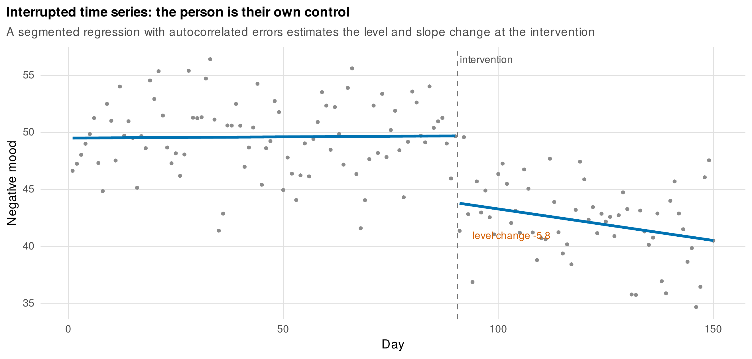
Note. One person’s daily negative mood (grey) with a segmented-regression fit (blue) before and after an intervention (dashed line, day ninety-one). The fit estimates a baseline level and slope, an immediate level change at the intervention, and a change in slope thereafter. Errors are modeled as first-order autoregressive.
The complication that distinguishes single-case time series from ordinary regression is that the errors are serially correlated, because consecutive daily moods are not independent, and ignoring that dependence has a specific and predictable consequence: the standard errors are understated, so the intervention looks more precisely estimated and more statistically significant than the data warrant. The remedy is to model the error autocorrelation, most simply by generalized least squares with a first-order autoregressive error structure, which estimates the residual autocorrelation jointly with the regression and inflates the standard errors to their honest size. Fitting the segmented model to mood_ts by generalized least squares recovers a level change of \(-5.85\) (against the planted \(-6\)) and a slope change of \(-0.057\) (against the planted \(-0.05\)), with an estimated residual autocorrelation of \(0.30\), and the point estimates are close to truth. The consequence of the autocorrelation is seen by comparing the two error treatments: ordinary least squares, which ignores the dependence, returns a standard error for the level change that is only three-quarters of the generalized-least-squares value, understating the uncertainty by a full quarter and correspondingly overstating the significance. The naive analysis would have reported a falsely precise effect.
The small-sample problem is more severe here than the point estimates suggest, and honesty requires stating it. With a baseline of ninety and a post-intervention segment of sixty, the series is at the upper end of what single-case studies achieve, yet the estimate of the error autocorrelation is itself uncertain, and at the shorter lengths typical of applied single-case work the generalized-least-squares standard errors, which treat the autocorrelation as known, are themselves optimistic. The remedies are a bootstrap that resamples the residual structure, or the small-sample corrections developed for exactly this design, and the reporting standard is to acknowledge the fragility rather than to present the asymptotic interval as final (Borckardt et al., 2008). Table 24.4 lays out the effect metrics and the inference options, including the nonoverlap effect sizes from the single-case design literature that complement the regression parameters and connect to the visual-analysis tradition (Parker et al., 2011).
Table 24.4. Interrupted time series: effect metrics and small-sample inference options.
| Quantity or option | What it estimates | Note for single-case use |
|---|---|---|
| Level change (\(\beta_2\)) | Immediate jump at the intervention | The discontinuity; report with an autocorrelation-corrected interval |
| Slope change (\(\beta_3\)) | Change in trajectory afterward | Accumulating effect; needs a long enough post phase to estimate |
| AR(1) error (\(\rho\)) | Residual serial dependence | Must be modeled; ignoring it understates all standard errors |
| GLS interval | Standard error treating \(\rho\) as known | Optimistic at short \(T\); the asymptotic default |
| Residual bootstrap | Resampled uncertainty | Preferred at short \(T\); respects the dependence structure |
| Nonoverlap effect sizes (Tau-U, NAP) | Distributional separation of phases | Complements the regression; links to visual analysis |
Note. Report the regression parameters with autocorrelation-corrected uncertainty, prefer a bootstrap to the asymptotic interval at short length, and treat visual analysis and statistical modeling as complementary rather than rival.
Common Pitfall • Four ways a single-subject time series misleads
First, estimating dynamics on a nonstationary series, so that a wandering mean is read as inertia and a trend as autocorrelation; check stationarity before interpreting any autoregressive coefficient. Second, over-identifying an ARMA model at short length, selecting a second moving-average term that fits the sample and will not replicate; keep the order low and corroborate the signature with an information criterion. Third, applying the Ljung-Box test without reducing its degrees of freedom by the number of fitted AR and MA parameters, which makes the whiteness check anticonservative and lets a misfit pass. Fourth, mistaking a bounded scale’s floor or ceiling for a dynamic, when a series pinned at the bottom of its range shows compressed variance and distorted autocorrelation that reflect the instrument, not the person; consider a transformation or a censoring-aware model, and never read a floor effect as regulation.
24.5 P-Technique and Person-Specific Structure
The idiographic analysis of structure, as opposed to dynamics, has a name and a history: P-technique factor analysis, introduced by Cattell in the nineteen-forties as one face of his data box, the three-way array of persons by variables by occasions (Cattell et al., 1947). The familiar factor analysis, R-technique, slices the box across persons at one occasion and asks how variables covary between people; P-technique slices it across occasions for one person and asks how that person’s variables covary over time. The output is a factor structure specific to the individual, an answer to the question of how this person’s affective states organize themselves, which need not match the structure that describes how people differ from one another. Nesselroade and Ford (1985) and Jones and Nesselroade (1990) developed the technique for lifespan and personality research precisely because the within-person organization is a distinct and often more relevant object than the between-person one.
Figure 24.9 applies P-technique to two people from affect_ema_items, factor-analyzing each person’s eight affect items across their occasions and displaying the loadings as heatmaps. The two structures differ. For one person the negative-affect items load cleanly on one factor and the positive-affect items on another, the textbook two-dimensional affect structure; for the other the pattern is shifted, with items cross-loading differently, so that the same eight items organize into a recognizably different personal architecture. The factor congruence coefficients between the two people’s matched factors are \(0.76\) and \(0.92\), high for the second factor and only moderate for the first, quantifying a genuine heterogeneity of structure. That two people can have different affect structures is not measurement error; it is the finding, and it is the empirical face of the nonergodicity that Section 24.1 argued for. The between-person R-technique structure, estimated across people, would report a single average architecture that describes neither person exactly, which is the ergodicity cash-out made concrete (Molenaar, 2004; Fisher et al., 2018).
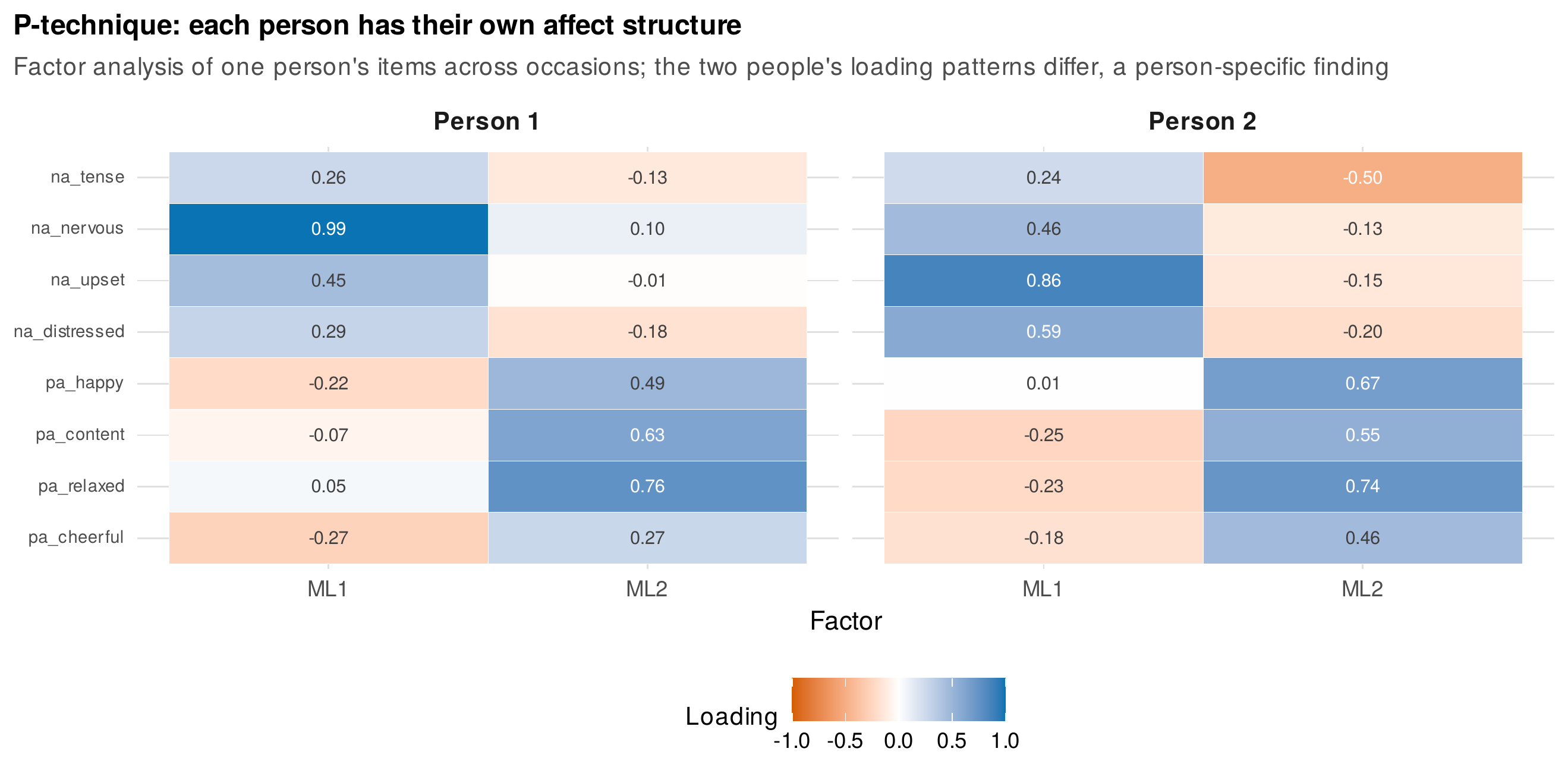
Note. Loading heatmaps from separate P-technique factor analyses of two people’s eight affect items across occasions in affect_ema_items. The two loading patterns differ, a person-specific finding: the same items organize into recognizably different personal structures, and a between-person analysis would report an average that fits neither exactly.
P-technique’s insight is real and its flaw is precise, and stating the flaw exactly is what motivates the next chapters. The technique factor-analyzes the occasions as though they were independent observations, exactly as R-technique treats persons, and thereby ignores the serial dependence that is the whole point of a time series. The consequence is not that the loadings are worthless, they are often roughly recoverable, but that the standard errors are wrong, because the effective number of independent observations is smaller than the occasion count, and that the technique says nothing about the dynamics, how the factors themselves evolve and predict one another over time. The repair is the dynamic factor model, which places a factor structure and a time-series structure in the same model, estimating person-specific factors that carry themselves and each other forward, and it is the subject of Chapter 26 (Hamaker et al., 2005; Molenaar, 2004). P-technique is thus best understood as the historically first and conceptually clearest statement of the idiographic-structure question, whose answer the state-space and dynamic-factor machinery of the following chapters supplies without its serial-dependence error.
24.6 How Long Must the Series Be?
The question that every reader with an intensive dataset must answer, and that the applied literature too often evades, is how many occasions the methods of this chapter actually require. The honest answer is not a single number but a function of the question asked, and it is best given by simulation rather than assertion, because the sampling behavior of these estimators at short length is exactly what the large-sample theory does not describe. The chapter therefore resources this section with a real simulation: stationary AR(1) series of length thirty, fifty, one hundred, and two hundred are generated with a known coefficient, the coefficient is re-estimated in each replication, and the bias, the root-mean-square error, and the width of the confidence interval are tabulated against series length.
The results, in Table 24.5 and Figure 24.10, are sobering and clarifying. At \(T=30\), the autoregressive coefficient is estimated with a downward bias of nearly a tenth, a root-mean-square error of \(0.19\), and a confidence interval \(0.65\) wide, so wide that it spans most of the admissible range and cannot distinguish a weakly persistent process from a strongly persistent one. Precision improves steadily with length: the root-mean-square error falls to \(0.13\) at \(T=50\), \(0.09\) at \(T=100\), and \(0.07\) at \(T=200\), and the interval narrows from \(0.65\) to \(0.49\) to \(0.34\) to \(0.24\). The downward bias, a known small-sample property of the autoregressive estimator, shrinks from nearly a tenth at \(T=30\) to about one part in a hundred at \(T=200\). The verdict is that an AR(1)-level question, estimating a single inertia coefficient to useful precision, is feasible at \(T\) of roughly fifty to one hundred, the reach of a two-week to one-month diary study at several beeps a day; but that a fine-grained question, a second-order oscillation, a moving-average term, or a full ARMA identification, needs considerably more, because each additional parameter is estimated from the same limited information and the identification itself becomes unstable at short length. The attenuation of the AR(2) fit in Section 24.3, \(0.38\) and \(-0.24\) recovered from generating values of \(0.55\) and \(-0.35\) at \(T=90\), is this table’s lesson in a single fit.
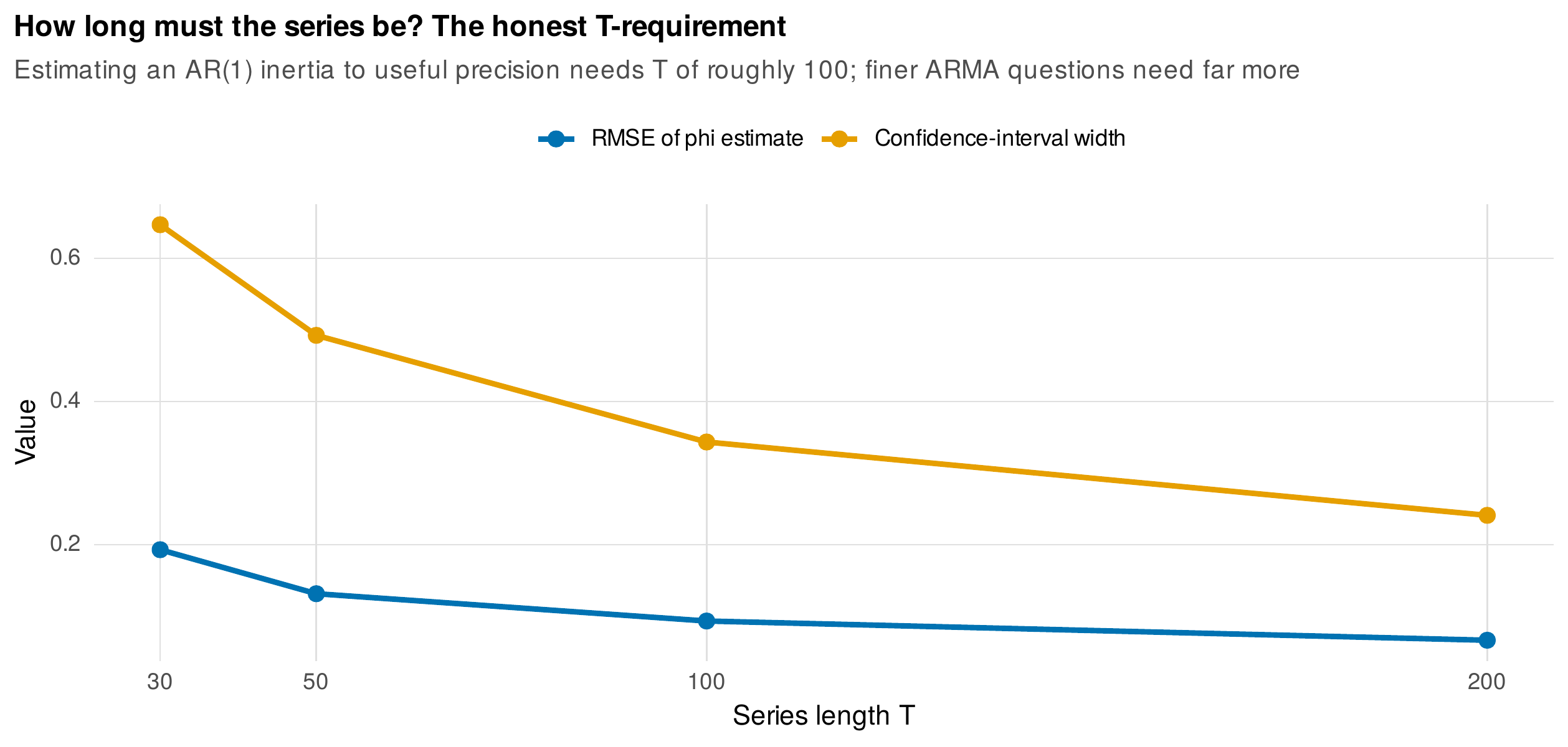
Note. Root-mean-square error (blue) and confidence-interval width (orange) for a first-order autoregressive coefficient, simulated against series length. Precision improves steadily with length; an inertia coefficient reaches useful precision near \(T=100\), while finer ARMA questions require substantially longer series.
Table 24.5. Series-length requirements: question type to honest minimum length.
| \(T\) | AR(1) bias | AR(1) RMSE | CI width | Verdict for the question type |
|---|---|---|---|---|
| 30 | \(-0.092\) | \(0.193\) | \(0.647\) | Too short for a trustworthy inertia estimate; interval spans most of the range |
| 50 | \(-0.047\) | \(0.132\) | \(0.492\) | Marginal for AR(1); adequate only for a strong, obvious effect |
| 100 | \(-0.027\) | \(0.093\) | \(0.343\) | Adequate for AR(1) inertia; the practical target for a diary study |
| 200 | \(-0.011\) | \(0.067\) | \(0.241\) | Good for AR(1); the floor for a credible AR(2) or ARMA question |
Note. Simulated bias, root-mean-square error, and ninety-five-percent interval width for a first-order autoregressive coefficient. An inertia question is feasible near \(T=100\); second-order and moving-average questions need more. The estimator is biased downward at short length, and the bias shrinks with \(T\).
This T-honesty is not a counsel of despair but the exact motivation for the chapters that follow. The field’s answer to the short-series problem is not to give up on the individual but to borrow strength across individuals, estimating each person’s dynamics while pooling information about the distribution of dynamics across the sample, which is the multilevel and dynamic-structural-equation machinery of Chapter 25. A person with only fifty occasions, too few to pin down their own oscillation, contributes to and benefits from a model that estimates the population of persons’ dynamics jointly, and their own estimate is stabilized by the shrinkage that pooling provides. The same two people whose AR(1) inertias were estimated here separately, ranging across the full ema_stress sample from essentially zero to above one-half with a mean near \(0.29\), become in Chapter 25 the random effects of a single model, and the heterogeneity that this chapter can only describe person by person becomes there a variance component to be estimated and explained.
24.7 Writing Up a Single-Subject Time-Series Analysis
Reporting an N=1 analysis credibly means making every analytic decision visible, because in a single-case study the decisions carry more weight than in a large sample and a reader cannot fall back on the law of large numbers to forgive them. The write-up should state the series length and the number and pattern of missing occasions, because these govern what can be estimated, and should report how the missingness was handled, whether by a likelihood that respects it or, if interpolation was used, with an acknowledgment of the autocorrelation it induces. It should document the stationarity assessment, the visual diagnosis and the ADF and KPSS results together, and any detrending or transformation applied, with the estimand that justified it. For the dynamics, it should report the identified order with the evidence for it, the autocorrelation and partial-autocorrelation signature and the information-criterion comparison, the fitted coefficients with their psychological reading, an inertia with its half-life, an oscillation with its period, and the residual diagnostic, the Ljung-Box result at the correct degrees of freedom, that certifies the model has whitened the series. For an interrupted time series, it should report the level and slope change with autocorrelation-corrected uncertainty, name the error structure, and confront the small-sample fragility rather than presenting the asymptotic interval as final. Throughout, the language should keep the psychological meaning attached to every number, because a coefficient reported without its meaning is uninterpretable, and it should state the generalization logic honestly, that a single person’s result is a single replication whose external validity rests on its recurrence in other persons, not on the significance of its own estimate.
A model paragraph reads: “One hundred eighty daily reports of negative mood were analyzed, with no missing occasions. The baseline segment (days 1 to 90) was stationary by visual inspection of the rolling mean and spread and by the ADF and KPSS tests (ADF \(=-7.02\), \(p<.01\); KPSS \(=0.05\), \(p>.10\)). The partial autocorrelation cut off after lag two, and an AR(2) model achieved the lowest AIC and BIC among the candidates considered. The fitted coefficients, \(\phi_1=0.38\) and \(\phi_2=-0.24\), imply a damped oscillation with a period of approximately 5.4 days, consistent with a regulatory dynamic that overshoots and returns; the residuals were white (Ljung-Box \(p=.93\), df corrected for the two estimated parameters). Given the series length, these second-order estimates should be read as attenuated, and the analysis is offered as one replication pending systematic replication across persons.” The practice box below distills the reporting standard into a checklist.
In Practice • Handling missed beeps, and a single-subject reporting checklist
Missed occasions are handled today by fitting on the observed data with a likelihood that respects the missingness, not by inventing values: base arima() accommodates internal missing values through its state-space likelihood, and the Kalman treatment of Chapter 26 is the principled general solution. Avoid mean-imputation and linear interpolation, which distort the autocorrelation. A single-subject report should state: (1) the series length and the number and pattern of missing occasions, with the missingness handling; (2) the stationarity assessment, visual and test-based, and any detrending or transformation with its estimand; (3) the identified order with its ACF/PACF and information-criterion evidence; (4) the fitted parameters with psychological interpretation, inertia with half-life, oscillation with period; (5) the residual whiteness diagnostic at corrected degrees of freedom; (6) for an ITS, the level and slope change with autocorrelation-corrected, and preferably bootstrapped, uncertainty; and (7) the replication logic for generalization, one person as one systematic replication, not a sample of one.
Chapter Summary
The single person measured densely over time is a legitimate object of analysis whose within-person structure need not match the between-person structure estimated across people, and the nonequivalence of the two levels is the intellectual charter of the idiographic program. Weak stationarity is the load-bearing precondition for every dynamic estimate, diagnosed first by the rolling mean and spread and second by the ADF and KPSS tests, whose opposite nulls are read jointly and whose power is low enough at psychological length that a small simulation is needed to state the fact, the ADF test rejecting a true unit-root alternative only about half the time at thirty occasions. The autoregressive coefficient is inertia, a psychological carryover with a half-life, not a nuisance to be corrected away, and a second-order autoregression with complex roots produces the damped oscillation that emotion researchers read as regulatory overshoot. The autocorrelation and partial-autocorrelation functions identify the order as signatures, corroborated at short length by information criteria that will otherwise overfit, and the fitted model is certified by a Ljung-Box test whose degrees of freedom must be reduced by the estimated parameters. Detrending and differencing remove a trend but answer different questions, and naive interpolation of missed occasions manufactures autocorrelation that a state-space treatment avoids. The interrupted time series makes the person their own control, estimating a level and a slope change against a baseline counterfactual with autocorrelated errors whose neglect understates every standard error, here by a quarter. P-technique factor analysis is the historical statement of the person-specific-structure question, insightful in its loadings and wrong in its standard errors because it ignores serial dependence, a flaw the dynamic factor model of Chapter 26 repairs. And the honest series-length requirement, an AR(1) inertia feasible near one hundred occasions and finer questions needing far more, is the exact motivation for the multilevel borrowing of Chapter 25, where the single person’s short series is stabilized by the population of persons around it.
Beltz, A. M., Wright, A. G. C., Sprague, B. N., & Molenaar, P. C. M. (2016). Bridging the nomothetic and idiographic approaches to the analysis of clinical data. Assessment, 23(4), 447–458. https://doi.org/10.1177/1073191116648209
Borckardt, J. J., Nash, M. R., Murphy, M. D., Moore, M., Shaw, D., & O’Neil, P. (2008). Clinical practice as natural laboratory for psychotherapy research: A guide to case-based time-series analysis. American Psychologist, 63(2), 77–95. https://doi.org/10.1037/0003-066X.63.2.77
Box, G. E. P., Jenkins, G. M., Reinsel, G. C., & Ljung, G. M. (2015). Time series analysis: Forecasting and control (5th ed.). John Wiley & Sons.
Cattell, R. B., Cattell, A. K. S., & Rhymer, R. M. (1947). P-technique demonstrated in determining psycho-physiological source traits in a normal individual. Psychometrika, 12(4), 267–288. https://doi.org/10.1007/BF02288941
Chatfield, C., & Xing, H. (2019). The analysis of time series: An introduction with R (7th ed.). Chapman and Hall/CRC. https://doi.org/10.1201/9781351259446
Fisher, A. J., Medaglia, J. D., & Jeronimus, B. F. (2018). Lack of group-to-individual generalizability is a threat to human subjects research. Proceedings of the National Academy of Sciences, 115(27), E6106–E6115. https://doi.org/10.1073/pnas.1711978115
Hamaker, E. L., Dolan, C. V., & Molenaar, P. C. M. (2005). Statistical modeling of the individual: Rationale and application of multivariate stationary time series analysis. Multivariate Behavioral Research, 40(2), 207–233. https://doi.org/10.1207/s15327906mbr4002_3
Hamilton, J. D. (1994). Time series analysis. Princeton University Press.
Jones, C. J., & Nesselroade, J. R. (1990). Multivariate, replicated, single-subject, repeated measures designs and P-technique factor analysis: A review of intraindividual change studies. Experimental Aging Research, 16(4), 171–183. https://doi.org/10.1080/03610739008253874
Kratochwill, T. R., Hitchcock, J., Horner, R. H., Levin, J. R., Odom, S. L., Rindskopf, D. M., & Shadish, W. R. (2010). Single-case designs technical documentation. What Works Clearinghouse. https://ies.ed.gov/ncee/wwc/Docs/ReferenceResources/wwc_scd.pdf
Kuppens, P., Allen, N. B., & Sheeber, L. B. (2010). Emotional inertia and psychological maladjustment. Psychological Science, 21(7), 984–991. https://doi.org/10.1177/0956797610372634
McCleary, R., McDowall, D., & Bartos, B. J. (2017). Design and analysis of time series experiments. Oxford University Press. https://doi.org/10.1093/oso/9780190661557.001.0001
Molenaar, P. C. M. (2004). A manifesto on psychology as idiographic science: Bringing the person back into scientific psychology, this time forever. Measurement: Interdisciplinary Research and Perspectives, 2(4), 201–218. https://doi.org/10.1207/s15366359mea0204_1
Molenaar, P. C. M., & Campbell, C. G. (2009). The new person-specific paradigm in psychology. Current Directions in Psychological Science, 18(2), 112–117. https://doi.org/10.1111/j.1467-8721.2009.01619.x
Nesselroade, J. R., & Ford, D. H. (1985). P-technique comes of age: Multivariate, replicated, single-subject designs for research on older adults. Research on Aging, 7(1), 46–80. https://doi.org/10.1177/0164027585007001003
Parker, R. I., Vannest, K. J., & Davis, J. L. (2011). Effect size in single-case research: A review of nine nonoverlap techniques. Behavior Modification, 35(4), 303–322. https://doi.org/10.1177/0145445511399147
Shumway, R. H., & Stoffer, D. S. (2017). Time series analysis and its applications: With R examples (4th ed.). Springer. https://doi.org/10.1007/978-3-319-52452-8
Suls, J., Green, P., & Hillis, S. (1998). Emotional reactivity to everyday problems, affective inertia, and neuroticism. Personality and Social Psychology Bulletin, 24(2), 127–136. https://doi.org/10.1177/0146167298242002
Velicer, W. F., & Fava, J. L. (2003). Time series analysis. In J. A. Schinka & W. F. Velicer (Eds.), Handbook of psychology: Research methods in psychology (Vol. 2, pp. 581–606). Wiley. https://doi.org/10.1002/0471264385.wei0223