Chapter 25
Vector Autoregression, Multilevel VAR, and Dynamic SEM
This is the flagship of Part VI, the chapter where the two threads that run the length of the book, the multivariate and the multilevel, are tied into a single knot. Chapter 24 taught the dynamics of one variable in one person; this chapter adds the other variables, so that the question becomes not how a mood carries itself forward but how a system of moods and stresses drives one another within the person over time, and then adds the other people, so that the dynamics themselves become random effects with a distribution across persons. The apparatus climbs in three deliberate steps on one dataset. The vector autoregression describes a single person’s system, its transition matrix a compact statement of who influences whom. Multilevel VAR lets that matrix vary across persons and estimates its average and its spread, recovering the temporal, contemporaneous, and between-person structure that a later chapter will dress as networks. Dynamic structural equation modeling completes the architecture by decomposing each observation into a latent person mean and a latent within-person process, which is what finally resolves the sample-mean centering bias flagged as far back as Chapter 13, and by making the autoregressions, the cross-lags, and even the innovation variances themselves random, distributions of dynamics rather than fixed numbers. The production standard for these models is Mplus, and its input is shown honestly; the estimation here is carried out with the tools at hand and with purpose-built simulations, so that every claim, the bias of sample-mean centering, the attenuation from measurement error, the accuracy bought by shrinkage, is auditable against a known truth rather than asserted.
Learning Objectives
After working through this chapter, you should be able to: (1) specify a VAR(1) for one person, read its transition matrix as autoregressive inertia on the diagonal and cross-lagged influence off it, judge stationarity from the eigenvalues, trace an impulse response, and state exactly what Granger prediction does and does not license; (2) specify multilevel VAR with person-specific transition matrices as random effects, distinguish its temporal, contemporaneous, and between-person matrices, and understand the two-stage versus joint estimation trade-off; (3) articulate the DSEM architecture, the latent decomposition into a between-person mean and a within-person process, random autoregressive, cross-lagged, and log-innovation-variance parameters, and the interval and missing-data handling; (4) explain why latent centering removes the sample-mean (Nickell and Lüdtke) bias and quantify that bias by series length; (5) read an Mplus DSEM analysis and its convergence diagnostics with the Bayesian literacy of Chapter 17; (6) navigate the bias landscape, sample-mean centering, measurement-error attenuation, random-effect shrinkage, and interval coarseness, with the remedy for each; and (7) choose among N=1 VAR, multilevel VAR, DSEM, and continuous-time models, and report a dynamic multilevel analysis with its required caveats.
25.1 One Person’s System: The Vector Autoregression
The vector autoregression generalizes the single-series autoregression of Chapter 24 to a vector of variables measured together over time. For a person observed on several variables at each occasion, collect the within-person deviations from that person’s own means into a vector \(\mathbf{y}_t\), and the first-order vector autoregression is \(\mathbf{y}_t = \boldsymbol{\Phi}\,\mathbf{y}_{t-1} + \boldsymbol{\varepsilon}_t\), where \(\boldsymbol{\Phi}\) is a square transition matrix and \(\boldsymbol{\varepsilon}_t\) is a vector of innovations with contemporaneous covariance \(\boldsymbol{\Sigma}\). The transition matrix is the object of interest, and its entries have sharp psychological readings. A diagonal entry \(\phi_{jj}\) is the carryover of variable \(j\), the same inertia the previous chapter named, the degree to which a variable’s own elevated state persists into the next occasion. An off-diagonal entry \(\phi_{jk}\) is a cross-lag, the degree to which variable \(k\) being elevated at one occasion predicts variable \(j\) at the next, over and above \(j\)’s own carryover. When two off-diagonal entries are both nonzero the system contains a feedback loop, each variable feeding the other forward in time, and the whole matrix is a compact statement of the person’s dynamic organization. Figure 25.1 labels the anatomy for a two-variable system of stress and negative affect.
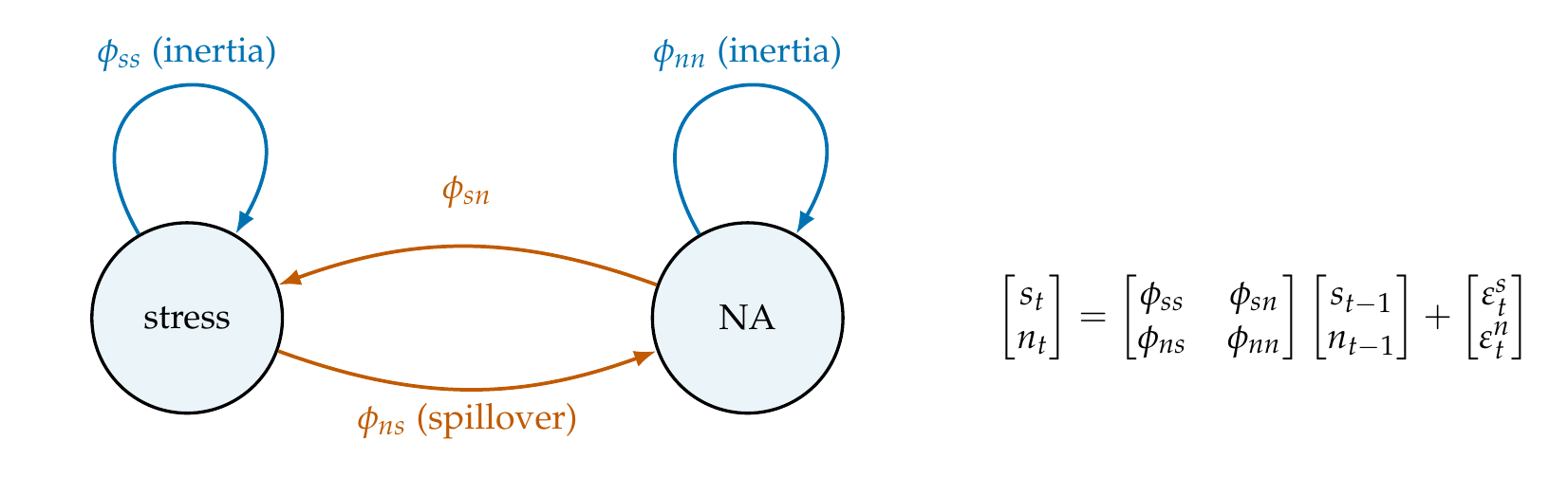
Note. A two-variable first-order vector autoregression. Diagonal coefficients (blue self-loops) are each variable’s inertia; off-diagonal coefficients (orange) are cross-lags, the lagged influence of one variable on the other. Two nonzero cross-lags make a feedback loop. The matrix equation on the right is the same statement in algebra.
Two properties govern whether such a system is well behaved. Stationarity, the precondition inherited from Chapter 24, now depends on the whole matrix rather than a single coefficient: the process is stationary when every eigenvalue of \(\boldsymbol{\Phi}\) lies strictly inside the unit circle of the complex plane, so that shocks decay rather than accumulate. Figure 25.2 shows the eigenvalues of a stable and an explosive two-variable system in the complex plane alongside the series each produces, the stable one fluctuating around its mean and the explosive one diverging without bound. The eigenvalues also carry the dynamics: real eigenvalues give smooth decay, complex eigenvalues give the damped oscillation the previous chapter met in the second-order autoregression, and the largest modulus sets the system’s overall persistence. The second property is the reading of the innovations. The contemporaneous covariance \(\boldsymbol{\Sigma}\) captures what the lagged structure did not predict, the shocks that arrive together at a single occasion, and its interpretation, whether a same-occasion association is a fast causal path or an unmodeled common cause, is deferred to the contemporaneous networks of Chapter 28; here it is a covariance to be estimated, not a claim to be made.
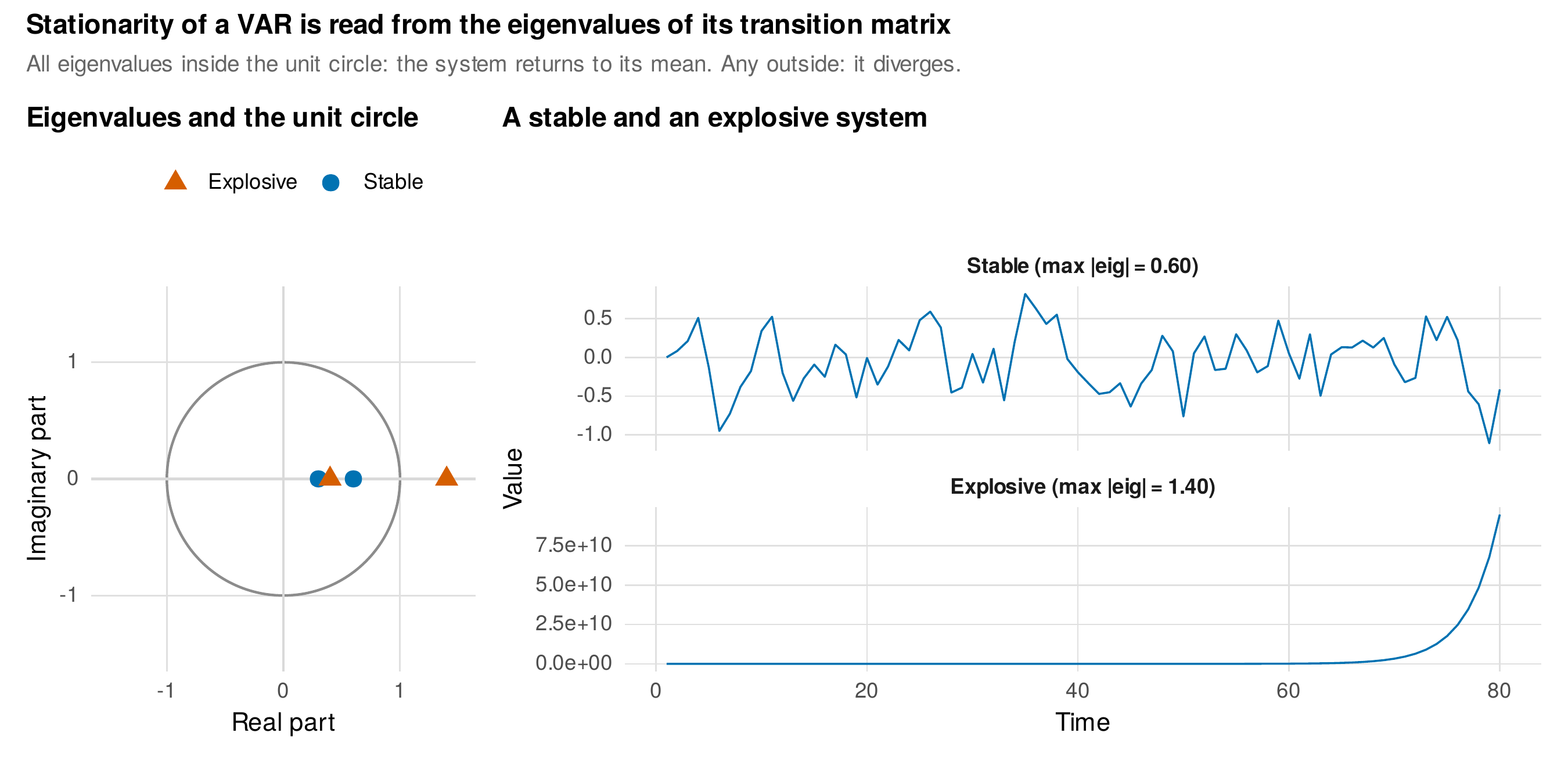
Note. Left: eigenvalues of a stable (blue) and an explosive (orange) transition matrix relative to the unit circle. Right: the series each system produces. All eigenvalues inside the circle means shocks decay and the system is stationary; an eigenvalue outside means the system diverges. The largest eigenvalue modulus summarizes overall persistence.
The dynamics of a fitted VAR are made vivid by the impulse-response function, which traces how a one-unit shock to one variable propagates through the system over subsequent occasions. Because the process is linear, the response at horizon \(h\) is \(\boldsymbol{\Phi}^{h}\) applied to the initial shock, and the resulting curves show both the decay of the shocked variable and its spillover into the others. Figure 25.3 shows the response to a stress shock in one person from the affect_ema data: stress decays from its impulse while negative affect rises to a delayed peak one occasion later and then subsides, the temporal signature of a spillover. The impulse-response reading is powerful but rests on assumptions that must be stated, linearity, stationarity, and an identification of which shock is primitive, and at psychological series lengths its sampling uncertainty is large, so it is best read qualitatively as the shape of a propagation rather than quantitatively as a precise forecast.
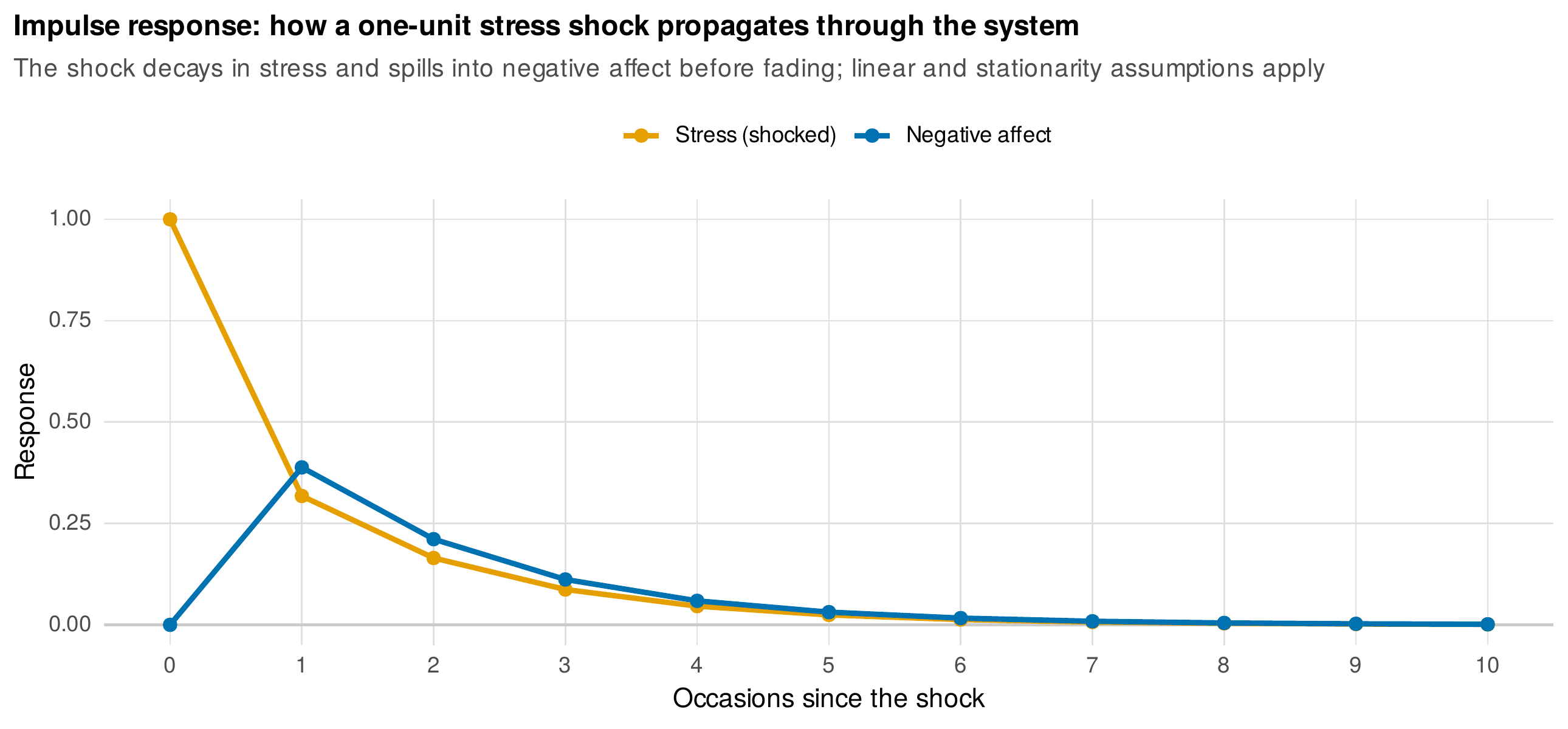
Note. The response of stress (orange) and negative affect (blue) over ten occasions following a one-unit shock to stress, for one affect_ema person. Stress decays; negative affect rises to a peak one occasion later before fading. The curves are \(\boldsymbol{\Phi}^{h}\) applied to the shock and assume linearity and stationarity.
Granger prediction deserves a precise statement because it is so often overread. A variable \(k\) Granger-causes a variable \(j\) if \(k\)’s past improves the prediction of \(j\) beyond what \(j\)’s own past provides, which is a statement about predictive content and nothing more. It is not evidence of a mechanism, because an omitted within-person variable that drives both can manufacture the predictive improvement, and it is dependent on the measurement interval, because a process that operates faster or slower than the sampling rate can appear or vanish. Fitted to one affect_ema person, lagged stress improves the prediction of negative affect beyond its own carryover, a significant Granger improvement, and the honest gloss is that the person’s stress carries predictive information about their next moment’s affect, not that stress was shown to cause it. The worked N=1 fit below estimates the transition matrix, checks its eigenvalues for stationarity, and runs the Granger test, and Table 25.1 collects the parameters with their psychological semantics.
# N=1 VAR(1) on one person: stress and negative affect
d1 <- subset(affect_ema, person == 59)
d1$cs <- d1$stress - mean(d1$stress, na.rm=TRUE)   # person-mean centering
d1$cn <- d1$na     - mean(d1$na,     na.rm=TRUE)
d1$Lcs <- c(NA, head(d1$cs, -1)); d1$Lcn <- c(NA, head(d1$cn, -1))
fit_s <- lm(cs ~ 0 + Lcs + Lcn, d1)      # stress equation
fit_n <- lm(cn ~ 0 + Lcs + Lcn, d1)      # negative-affect equation
Phi <- rbind(stress = coef(fit_s), na = coef(fit_n))   # transition matrix
Mod(eigen(Phi)$values)                    # all < 1 => stationary (max 0.53)
# Granger: does lagged stress add to predicting NA beyond NA's own lag?
anova(lm(cn ~ 0 + Lcn, d1), lm(cn ~ 0 + Lcn + Lcs, d1))   # p = 0.021
Table 25.1. VAR parameters and their psychological semantics.
| Parameter | Statistical meaning | Psychological semantics |
|---|---|---|
| \(\phi_{jj}\) (diagonal) | Lagged effect of a variable on itself | Inertia or carryover of variable \(j\); its resistance to returning to baseline |
| \(\phi_{jk}\) (off-diagonal) | Lagged effect of \(k\) on \(j\) | Spillover or transmission: \(k\) now forecasts \(j\) next, beyond \(j\)’s own carryover |
| Eigenvalues of \(\boldsymbol{\Phi}\) | Spectrum of the transition matrix | Inside unit circle: stable regulation; complex: oscillation; largest modulus: overall persistence |
| \(\boldsymbol{\Sigma}\) (innovations) | Contemporaneous covariance of shocks | What arrives together and was not predicted; same-occasion coupling (network reading in Ch 28) |
| Impulse response \(\boldsymbol{\Phi}^{h}\) | System response to a unit shock | How a perturbation propagates and spills over before decaying |
| Granger improvement | Predictive gain from another series’ past | Predictive, not causal; interval-dependent; vulnerable to omitted within-person confounders |
Note. Every coefficient carries a within-person reading. The diagonal is inertia, the off-diagonal is transmission, the eigenvalues govern stability and oscillation, and Granger content is prediction, not mechanism.
The reason one person’s VAR is only the starting point is that the transition matrix is not the same for everyone. Fitting the same reduced-form VAR to a sample of affect_ema persons and reading off one coefficient, the lagged effect of stress on next-moment negative affect, produces Figure 25.4: the estimates scatter widely across people, some strongly reactive and some barely, and each person’s estimate carries a wide confidence interval because a single person supplies only a few dozen usable transitions. The spread is the phenomenon, the same lesson as the random slopes of Chapter 23, and the wide intervals are the problem, the same short-series limitation as Chapter 24. Both point to the same move: model the person-specific matrices as random effects and borrow strength across people, which is multilevel VAR.
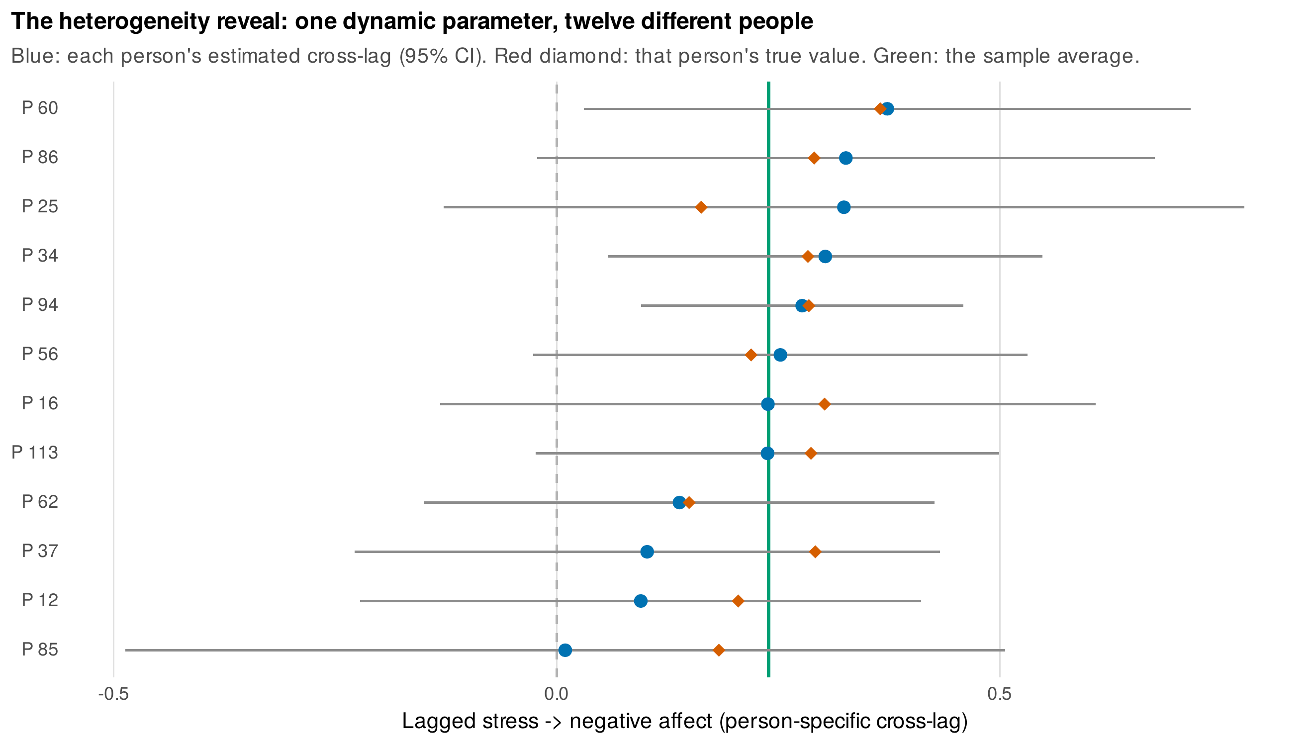
Note. Each person’s estimated lagged effect of stress on negative affect (blue point) with its 95% confidence interval, twelve affect_ema persons, the true value for each (red diamond), and the sample average (green line). The dynamics differ across people, and each single-person estimate is imprecise, the two facts that motivate multilevel pooling.
Foundations Box • The VAR stationary distribution and the sample-mean bias
A stationary VAR(1) has a stationary distribution whose covariance \(\boldsymbol{\Gamma}_0\) satisfies the discrete Lyapunov equation \(\boldsymbol{\Gamma}_0 = \boldsymbol{\Phi}\,\boldsymbol{\Gamma}_0\,\boldsymbol{\Phi}^{\top} + \boldsymbol{\Sigma}\), the multivariate generalization of the AR(1) variance \(\sigma^2_\varepsilon/(1-\phi^2)\); solving it gives the process variance implied by the dynamics and the innovation covariance together, and its existence requires the eigenvalues of \(\boldsymbol{\Phi}\) inside the unit circle. The lagged autocovariance is \(\boldsymbol{\Gamma}_1 = \boldsymbol{\Phi}\,\boldsymbol{\Gamma}_0\), so the transition matrix is recovered as \(\boldsymbol{\Phi} = \boldsymbol{\Gamma}_1 \boldsymbol{\Gamma}_0^{-1}\), the multivariate Yule-Walker relation. The catch, central to this chapter, is that the deviations \(\mathbf{y}_t\) are formed by subtracting each person’s mean, and that mean is not known but estimated from the same short series. The estimated mean is pulled toward the very observations it will be subtracted from, so the centered deviations are slightly negatively correlated with their own past by construction, and the autoregression is biased downward. This is the Nickell (1981) bias in its dynamic-panel guise and the Lüdtke et al. (2008) contextual-effect bias in its multilevel guise, one phenomenon with two names, and it is the reason a latent treatment of the person mean, deferred to Section 25.3, is worth the machinery it costs.
25.2 Multilevel VAR
Multilevel VAR treats each person’s transition matrix as a draw from a population of transition matrices. The within-person model is the vector autoregression of the previous section; the multilevel layer makes each person’s autoregressive and cross-lagged coefficients random effects, with fixed effects that estimate the average dynamics and random-effect variances that estimate their heterogeneity, exactly the random-slope logic of Chapter 23 applied now to lagged predictors and to several equations at once. The estimation produces three matrices, and keeping them distinct is essential. The temporal matrix is the fixed-effect transition matrix, the average lagged dynamics. The contemporaneous matrix is the partial-correlation structure of the within-person innovations, the same-occasion associations that remain after the lagged structure is removed. The between-person matrix is the covariance of the person means, how people who are higher on one variable on average tend to sit on the others. These are the three network layers that Chapter 28 will interpret as graphs; here they are statistical objects to be estimated and, because affect_ema was generated from a known multilevel VAR, to be checked against their truth.
That check is the chapter’s most satisfying exhibit. Figure 25.5 places the estimated temporal, contemporaneous, and between-person matrices beside the data-generating values, each cell showing the multilevel estimate with the truth beneath it. The temporal matrix recovers the planted structure: the diagonal inertias near their generating values, the lagged spillover of stress into negative affect at \(0.24\) against a true \(0.24\), and the near-zero entries where the truth is zero. The diagonal estimates sit slightly below their true values, the visible fingerprint of the sample-mean bias derived in the foundations box, an average carryover recovered as \(0.31\) where the truth is \(0.35\). The contemporaneous matrix recovers the positive stress-affect coupling and the negative affect-positive-affect coupling; the between-person matrix recovers the correlations of the person means. An estimator that reproduces a known transition matrix, a known innovation structure, and a known between-person structure from noisy, missing, bounded data is one a reader can trust on data whose truth is unknown.
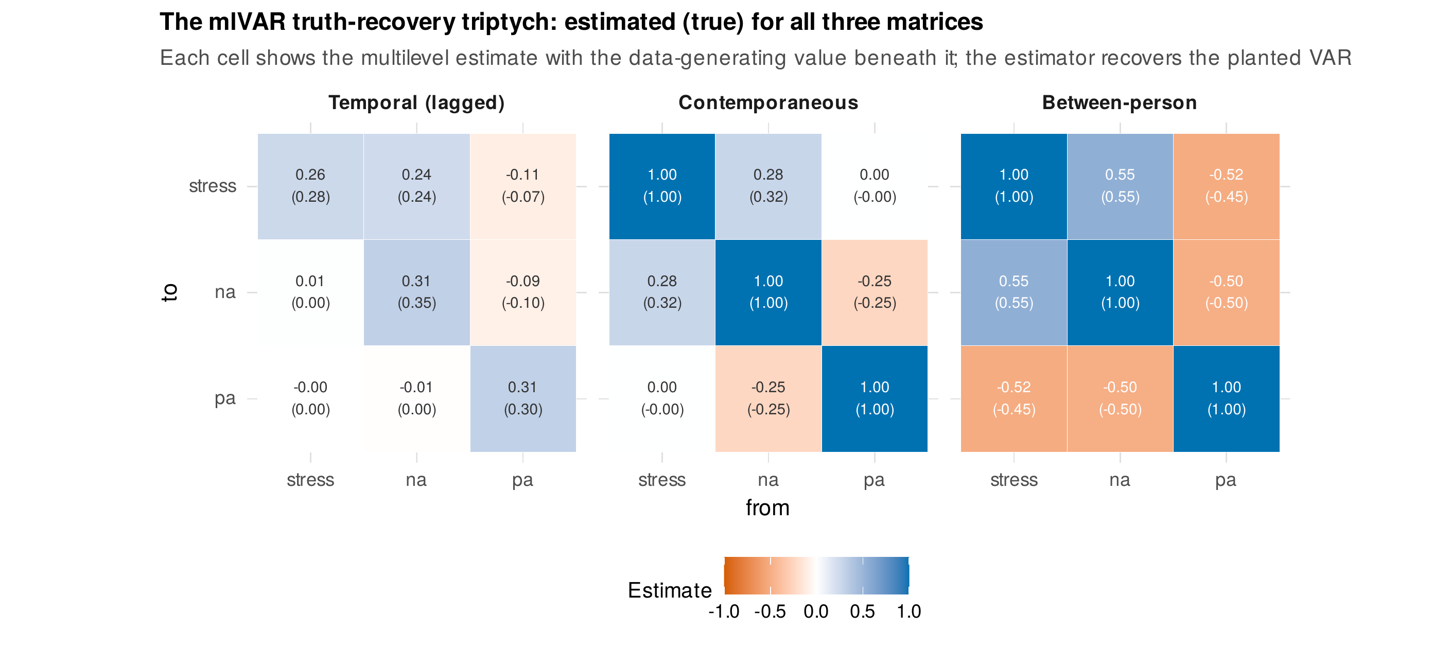
Note. Estimated (and, in parentheses, true) entries of the temporal, contemporaneous, and between-person matrices from a multilevel VAR fit to affect_ema, whose data-generating process is a known multilevel VAR. Fill encodes the estimate. The estimator recovers all three matrices; the diagonal temporal entries sit slightly low, the sample-mean bias of the foundations box.
There are two routes to these estimates, and the contrast between them is the conceptual ladder to DSEM. The transparent route is two-stage: fit a separate VAR to each person, then pool the person-specific coefficients by averaging or meta-analysis. It is easy to explain and easy to compute, but it is biased when series are short, because each person’s estimate carries the small-sample bias of the previous section and the meta-analytic step treats those noisy estimates as if they were precise. The better route is joint estimation, fitting all persons together in one multilevel model so that each person’s dynamics are estimated with the population as a prior, which shrinks noisy person-specific estimates toward the average and improves their accuracy. Figure 25.6 shows the payoff: the raw per-person cross-lags scatter widely around their true values, while the shrunken multilevel estimates cluster closer to the truth line, and the root-mean-square error falls from \(0.142\) to \(0.088\), a substantial gain bought entirely by borrowing strength. The shrunken estimates are visibly flatter than the raw ones, deliberately so, because when a person’s own data are too thin to pin down their dynamics, the honest estimate is pulled toward what the population says is likely. The package ecosystem for multilevel VAR fits this model nodewise, one multilevel regression per variable, which is the workflow the run-it-in-R panel sketches.
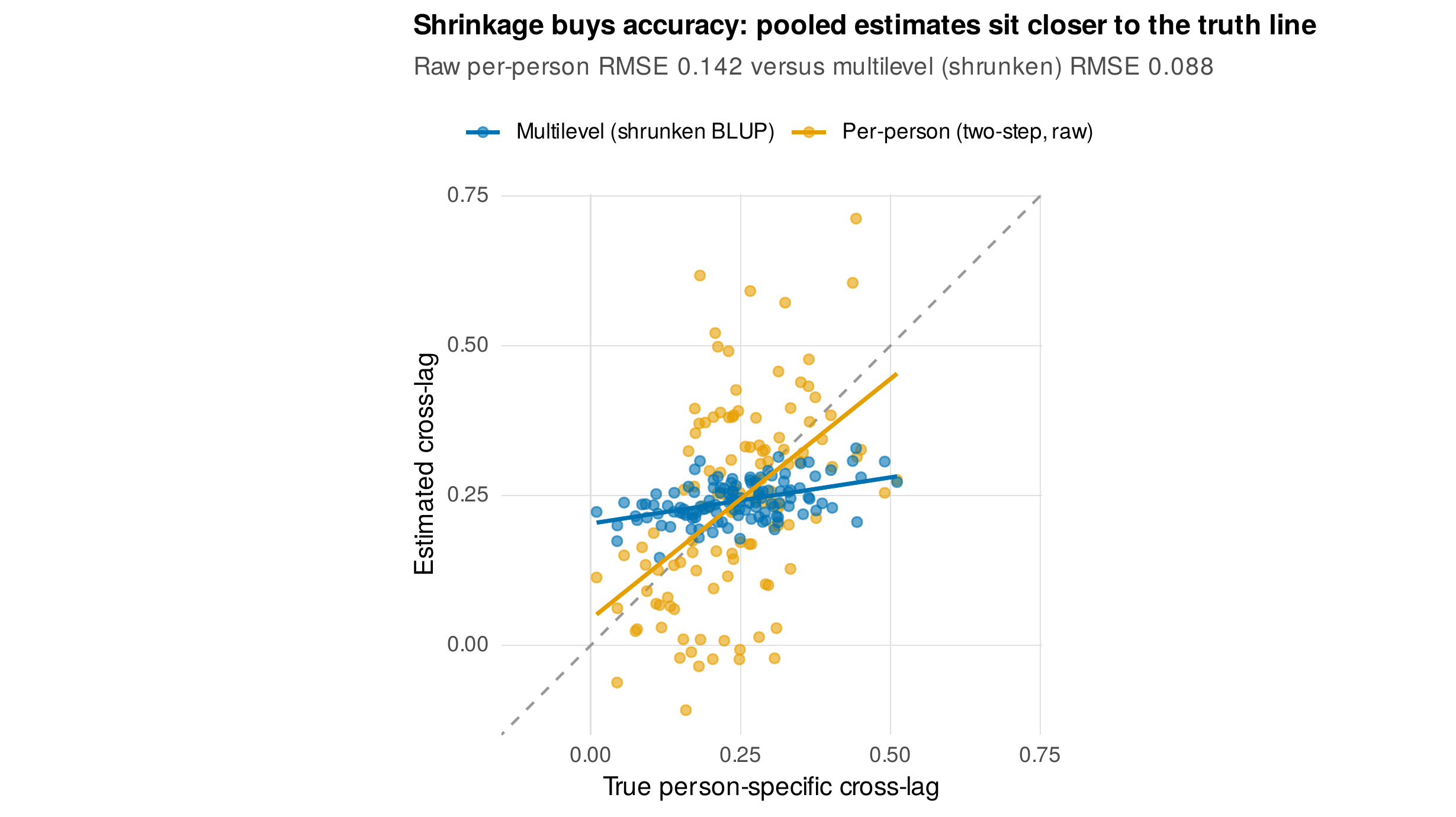
Note. Person-specific cross-lags plotted against their true values: raw per-person (two-step) estimates in orange, multilevel shrunken estimates in blue, with the dashed line marking perfect recovery. Shrinkage pulls the noisy per-person estimates toward the population and lowers the root-mean-square error from \(0.142\) to \(0.088\).
# Multilevel VAR, nodewise (one multilevel regression per variable).
# Person-mean-center each variable and its lag first (columns c_*, Lc_*).
library(lme4)
m_na <- lmer(c_na ~ Lc_stress + Lc_na + Lc_pa +
                    (1 + Lc_na + Lc_stress | person), data = d)
fixef(m_na)                       # a row of the temporal matrix (avg dynamics)
coef(m_na)$person[, "Lc_stress"]  # person-specific cross-lags (shrunken BLUPs)
# contemporaneous: partial correlations of the nodewise residuals
# between-person: correlations of the person means
Table 25.2. Two-step, multilevel VAR, and DSEM compared.
| Feature | Two-step per-person | Multilevel VAR | DSEM |
|---|---|---|---|
| Centering | Sample mean | Sample mean | Latent (unbiased) |
| Person dynamics | Independent fits | Random effects, shrunken | Random effects, shrunken |
| Small-\(T\) bias | Full Nickell bias | Nickell bias remains | Removed by latent mean |
| Measurement error | Attenuates \(\phi\) | Attenuates \(\phi\) | Repairable via latent indicators |
| Innovation variance | Per person, ad hoc | Usually fixed or random | Random (log scale) |
| Missing data | Listwise on pairs | Available pairs | Model-based (Kalman) |
| Estimation | OLS then pool | (RE)ML, nodewise | Bayesian (MCMC) |
| Typical software | any | mlVAR | Mplus, dynr, Stan |
Note. The three approaches ascend in what they correct. Two-step is transparent but biased; multilevel VAR adds shrinkage but keeps the sample-mean bias; DSEM adds latent centering, latent measurement, model-based missingness, and random innovation variance at the cost of Bayesian machinery.
25.3 Dynamic Structural Equation Modeling
Dynamic structural equation modeling is the multilevel VAR rebuilt on a latent-variable foundation, and its defining move is a decomposition. Each observed score is written as the sum of a between-person part and a within-person part, \(y_{it} = \mu_i + \tilde{y}_{it}\), where \(\mu_i\) is the person’s latent mean, a random effect at the between level, and \(\tilde{y}_{it}\) is the latent within-person deviation that carries the serial dynamics. The autoregression and cross-lags operate on the latent \(\tilde{y}\), not on the observed score minus a sample average, and this is precisely what removes the bias of the foundations box: because \(\mu_i\) is a parameter estimated with information borrowed across persons rather than a within-person sample mean, the deviations are not mechanically correlated with their own past, and the dynamics are recovered without the downward pull. Figure 25.7 draws the architecture, the between level supplying each person’s latent mean and their person-specific dynamic parameters, the within level running the vector autoregression on the latent deviations.
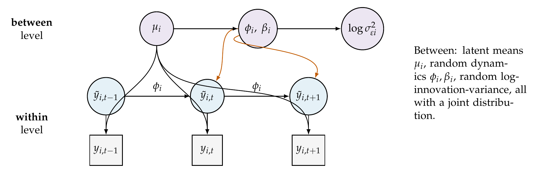
Note. Each observed score \(y_{it}\) is the sum of a latent person mean \(\mu_i\) (between level) and a latent within-person deviation \(\tilde{y}_{it}\) (within level) that carries the autoregressive and cross-lagged dynamics. The dynamic parameters \(\phi_i,\beta_i\) and the log-innovation-variance are themselves random effects with a joint between-person distribution. Latent centering on \(\mu_i\), rather than on a sample mean, is what removes the small-sample bias.
The payoff of latent centering is quantified in Figure 25.8, the chapter’s methodological centerpiece. A two-level autoregression with a known coefficient of \(0.40\) is estimated three ways at increasing series length: by subtracting each person’s observed mean, by subtracting the person’s true mean, an oracle no analyst has, and by treating the mean as a latent parameter in a hierarchical Bayesian model, which is what DSEM does. Sample-mean centering is badly biased downward at short series, recovering \(0.23\) at ten occasions and \(0.32\) at twenty, and only creeps toward the truth as the series lengthens. Oracle centering is unbiased at every length. Latent centering tracks the oracle closely, removing almost all of the bias even at twenty occasions, with only a small upward wobble at the extreme of ten occasions where the between and within parts are barely separable. The lesson is direct: at the series lengths psychology actually collects, sample-mean centering understates every autoregression and cross-lag, and the latent decomposition is the practical fix.
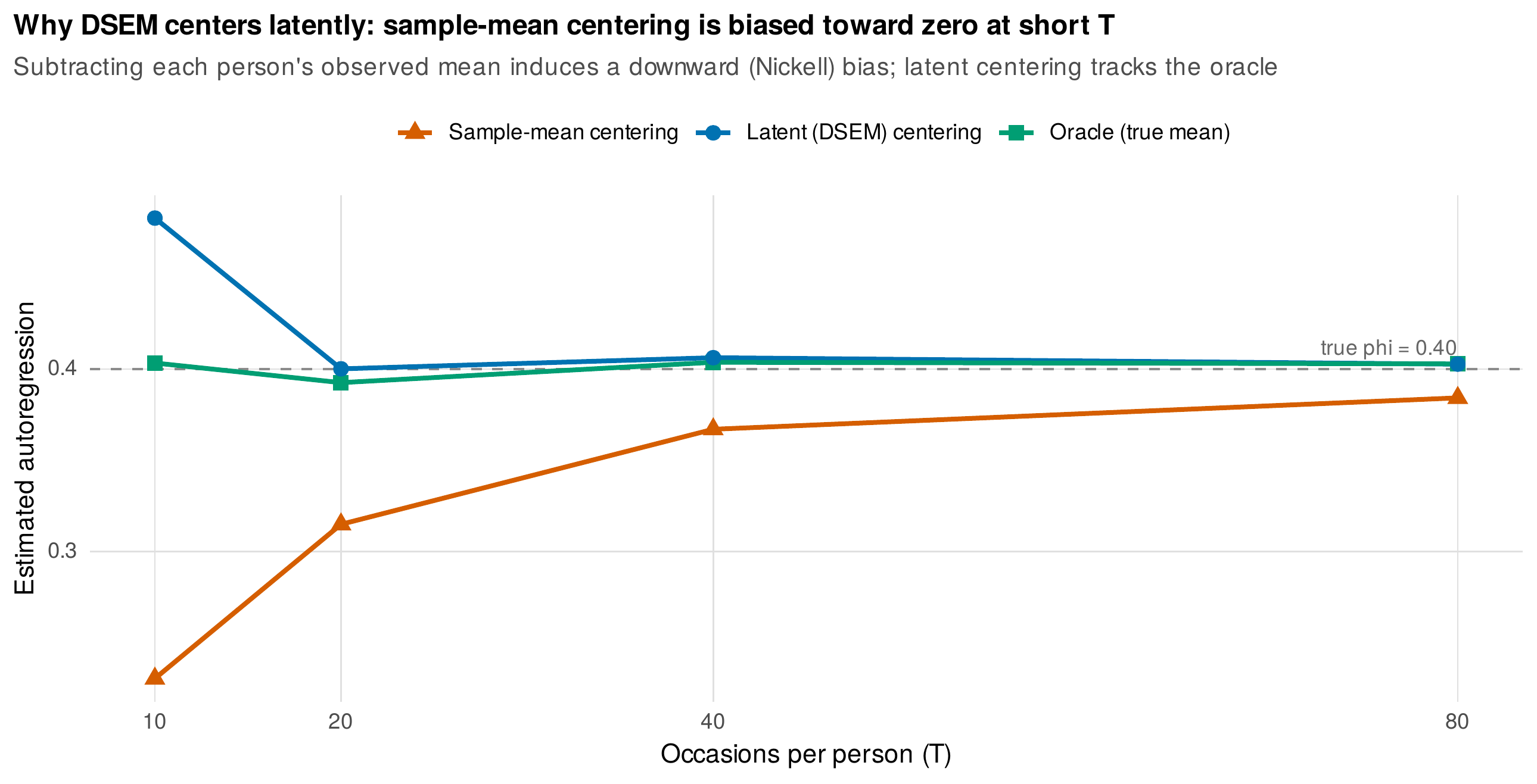
Note. An autoregression with true value \(0.40\) estimated by sample-mean centering (orange), oracle true-mean centering (green), and latent hierarchical centering (blue), against series length. Sample-mean centering is biased toward zero at short series; latent centering tracks the oracle. The gap is the bias DSEM removes.
The architecture buys three further capabilities. The dynamic parameters are random, so DSEM estimates not a single transition matrix but a distribution of them, and it can ask whether a person’s dynamics covary with their mean level, whether, for instance, people who are more stressed on average also transmit stress into affect more strongly. Figure 25.9 shows the distribution of person-specific cross-lags across the sample and their relationship to mean stress level, which in these data is essentially null, itself a finding, that spillover strength and average level are separate individual differences. The innovation variance is also allowed to be random, on the log scale, so that people differ not only in their dynamics but in their moment-to-moment volatility, which is the location-scale idea of Chapter 16 reborn in a dynamic model. Figure 25.10 shows the spread of person-specific innovation standard deviations, the volatility that a fixed-variance model would wrongly assume constant. And the measurement layer can be made latent: a DSEM with multiple indicators per construct estimates the dynamics of a latent factor rather than of a single fallible item, which matters because measurement error attenuates autoregressive estimates toward zero. Figure 25.11 demonstrates that attenuation, an autoregression of \(0.50\) recovered as \(0.38\) at a reliability of \(0.8\) and as \(0.23\) at a reliability of \(0.5\), and the multiple-indicator DSEM is the repair, the P-technique of Chapter 24 redeemed at scale and equipped with the serial structure it lacked.
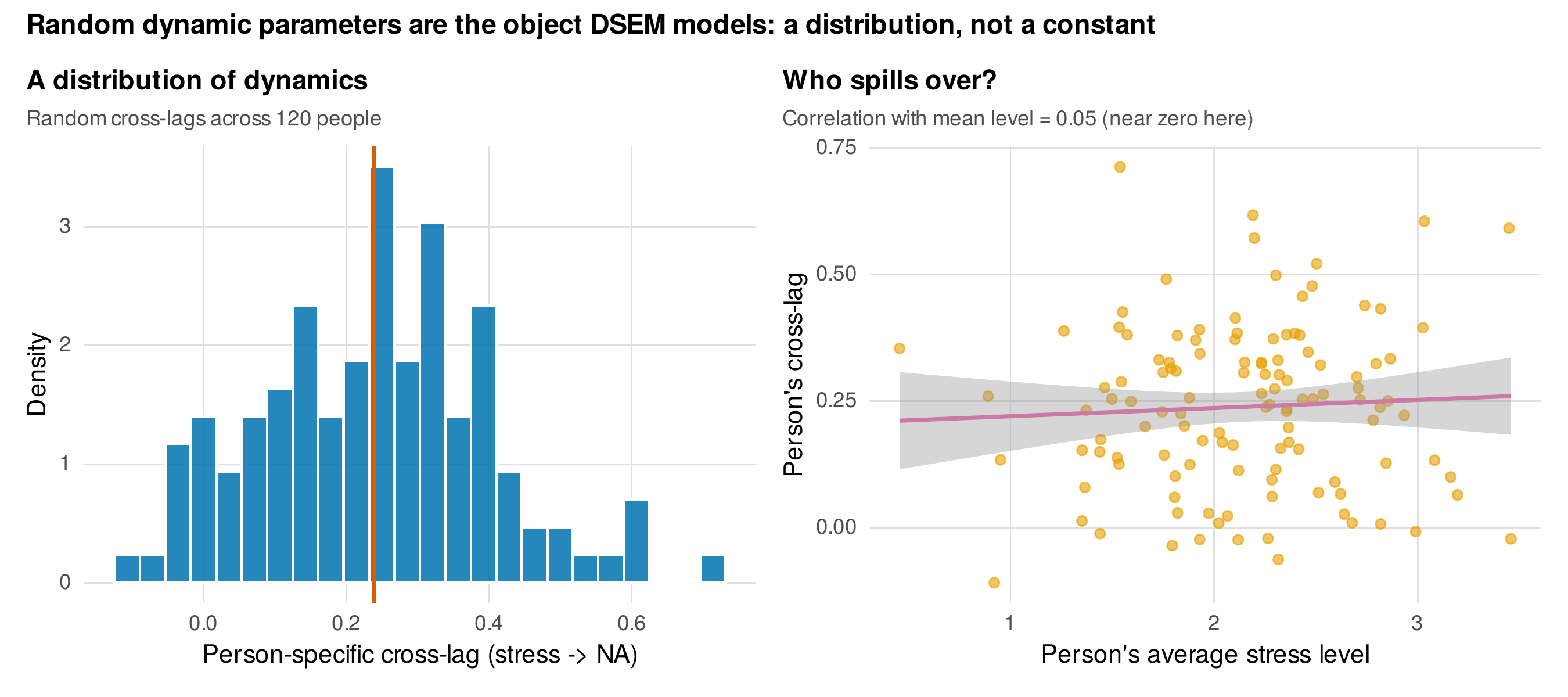
Note. Left: the distribution of person-specific cross-lags (stress into negative affect) across 120 people, with the average marked. Right: those cross-lags against each person’s average stress level; the near-zero correlation says spillover strength and mean level are distinct individual differences in these data. DSEM models this distribution directly.
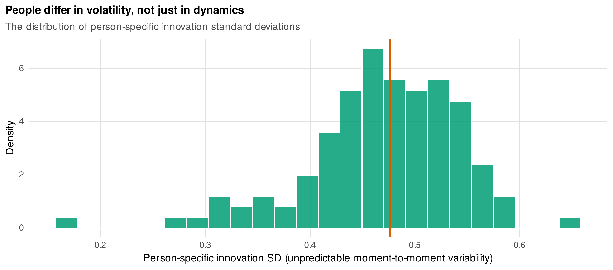
Note. The distribution of person-specific innovation standard deviations, the size of the unpredictable moment-to-moment shocks. DSEM lets this vary across people as a random log-innovation-variance, the location-scale model of Chapter 16 carried into the dynamic setting.
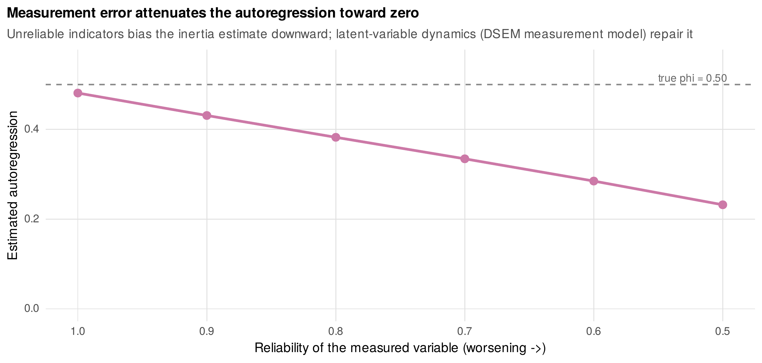
Note. The estimated autoregression as a single fallible indicator’s reliability declines, with the true value \(0.50\) marked. Unreliable measurement biases the inertia estimate toward zero; a multiple-indicator DSEM that models a latent construct repairs the attenuation.
The estimation is Bayesian, and for good reason: the latent decomposition, the random dynamics, and the random variances together make the likelihood difficult for maximum-likelihood methods, whereas Markov chain Monte Carlo handles the latent means and random effects naturally. In practice the field standard is Mplus, whose DSEM implementation reads intensive longitudinal data, decomposes it into the latent within and between parts, places priors on the parameters, and returns posterior summaries with convergence diagnostics in the Bayesian dialect of Chapter 17, the potential scale reduction factor in place of the R-hat named there but the same quantity. The input below specifies the stress-to-affect spillover model with random cross-lags; the &1 notation forms the lag, the vertical bar names a random slope, and the TINTERVAL option discretizes the unequal spacing between beeps, the bridge to Chapter 27’s continuous-time treatment. Table 25.3 translates the settings into the decisions they encode.
! Mplus two-level DSEM: random AR and random stress->NA cross-lag
VARIABLE:  NAMES = person day beep stress na pa;
           USEVARIABLES = stress na;
           CLUSTER = person;             ! persons are the clusters
           LAGGED = stress(1) na(1);     ! form lag-1 predictors
           MISSING = ALL(-999);
ANALYSIS:  TYPE = TWOLEVEL RANDOM;
           ESTIMATOR = BAYES;            ! MCMC; ML struggles here
           PROCESSORS = 2;
           BITERATIONS = (2000);         ! minimum; grow until PSR settles
MODEL:
  %WITHIN%
    phi  | na     ON na&1;               ! random AR of negative affect
    beta | na     ON stress&1;           ! random cross-lag: stress -> NA
    phis | stress ON stress&1;           ! random AR of stress
  %BETWEEN%
    na WITH stress;                      ! between-person mean covariance
    phi beta phis WITH na stress;        ! do dynamics covary with level?
OUTPUT:    TINTERVAL STANDARDIZED;
Table 25.3. DSEM settings in Mplus and the decisions they encode.
| Setting | What it controls | Guidance |
|---|---|---|
ESTIMATOR = BAYES | MCMC estimation | Required; ML cannot handle the latent decomposition with random dynamics |
BITERATIONS | Number of MCMC iterations | Set a minimum and grow until the scale-reduction factor stabilizes; do not accept the default uncritically |
| Priors | Prior distributions on parameters | Defaults are weakly informative; report them and run a sensitivity check on any that matter |
| Scale-reduction factor | Convergence diagnostic | The Mplus name for R-hat (Ch 17); values near \(1.0\) indicate convergence; inspect trace plots |
LAGGED, &1 | Lag construction | Lags are within cluster; verify they respect the intended time structure |
TINTERVAL | Interval discretization | Aligns unequal spacing to a grid; coarse grids distort dynamics (Section 25.4; Ch 27) |
Note. DSEM inherits the Bayesian workflow of Chapter 17. Convergence is judged by the scale-reduction factor and trace plots, iterations are grown until it settles, and priors are reported and probed rather than accepted silently.
Common Pitfall • Four ways a dynamic multilevel analysis is over-read
First, reading a cross-lag as a within-person causal effect, when it is a predictive association vulnerable to omitted within-person confounders and dependent on the measurement interval; the honest claim is prediction, and the causal language belongs only to a design that earns it. Second, comparing transition matrices across persons or groups without invariance thinking, when the coefficients may be on different within-person scales; standardize deliberately, and prefer a within-person standardization whose meaning is stated, because the unstandardized and standardized cross-lags answer different questions. Third, ignoring the discretization of unequal intervals, so that a coefficient estimated across beeps of different real duration is interpreted as a single lag effect; state the interval and, when spacing varies badly, move to continuous time (Chapter 27). Fourth, treating a person-specific DSEM estimate as that person’s unvarnished truth, when it is a posterior shrunken toward the population; the shrinkage is a feature, but it means the estimate speaks partly for the sample, and extreme individual claims should be made cautiously.
Software Note • The dynamic-modeling software landscape
This landscape moves quickly, and the honest matrix is as follows. For a single person’s VAR, base tools and the vars package suffice. For multilevel VAR, the mlVAR package estimates the temporal, contemporaneous, and between matrices nodewise and pairs naturally with the network displays of Chapter 28; graphicalVAR estimates the regularized within-person version. For full DSEM, with latent centering, random dynamics, random innovation variances, latent measurement, and model-based missingness, Mplus is the production standard through the MplusAutomation round-trip, and Bayesian implementations in Stan and the dynr package for state-space dynamics cover much of the same ground in R with more assembly required. The analyses in this chapter were fit with base tools, lme4 for the multilevel VAR, and purpose-built simulations and a small hand-written Gibbs sampler for the DSEM mechanisms, so that the latent-centering bias, the shrinkage gain, and the measurement-error attenuation could each be shown against a known truth rather than taken on faith. Readers with production needs should reach for Mplus or a Stan implementation; readers who want to understand what those engines do will find the mechanisms reproduced in the shipped scripts.
25.4 The Bias Landscape
The value of the preceding machinery is clearest when its failure modes are gathered in one place, because each is a specific bias with a specific remedy, and a practitioner who knows the landscape can anticipate which way an estimate is wrong before collecting a single datum. Four biases have appeared in this chapter, each demonstrated by simulation against a known truth. Sample-mean centering biases the autoregression downward at short series, by nearly half at ten occasions and by a tenth even at forty, and the remedy is latent centering. Measurement error attenuates the autoregression toward zero in proportion to unreliability, and the remedy is a latent measurement model. Two-step estimation inflates the apparent heterogeneity of dynamics because it treats noisy person-specific estimates as precise, and the remedy is joint estimation with shrinkage. And interval coarseness, treating unequally spaced occasions as though they were evenly spaced, biases the dynamics because transitions of different real duration are pooled into one coefficient. Figure 25.12 demonstrates the last of these: a continuous-time process whose true one-step autoregression is \(0.67\) is estimated at \(0.56\) by a naive equal-interval fit, a downward bias of a tenth, and is recovered at \(0.66\) once the intervals are respected, the continuous-time correction of Chapter 27. Table 25.4 states each bias, what drives its magnitude, and its remedy, and Table 25.5 gives honest series-length and sample-size guidance for the questions this chapter’s models are asked to answer.
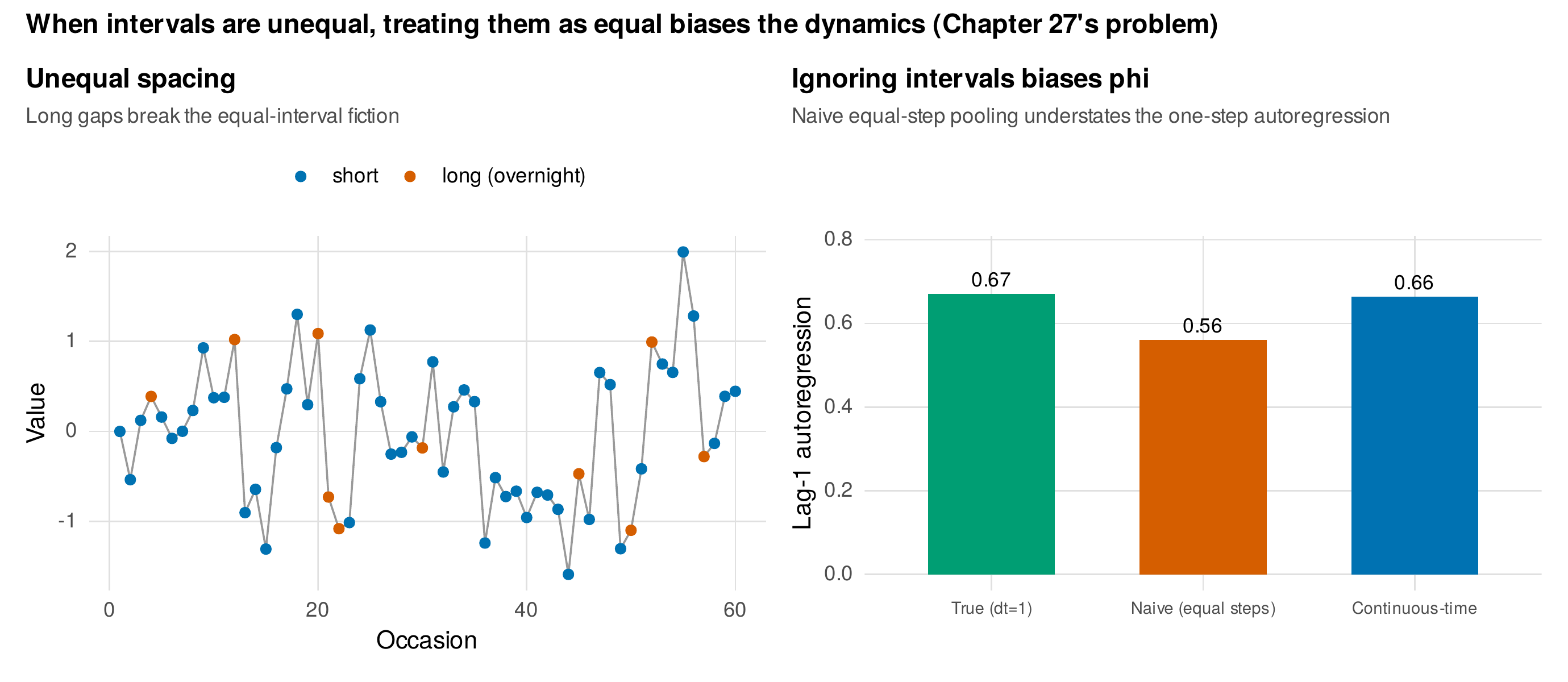
Note. Left: a continuous-time process sampled at unequal intervals, with the long (overnight) gaps marked. Right: the true one-step autoregression (\(0.67\)), the biased naive equal-interval estimate (\(0.56\)), and the continuous-time recovered value (\(0.66\)). Ignoring the spacing understates the autoregression; Chapter 27 models it directly.
Table 25.4. The bias landscape: issue, magnitude drivers, and remedy.
| Bias | Direction | Magnitude driver | Remedy |
|---|---|---|---|
| Sample-mean centering | Toward zero | Short \(T\); small between-person variance | Latent centering (DSEM) |
| Measurement error | Toward zero | Low reliability of the indicator | Latent measurement model (multi-indicator DSEM) |
| Two-step heterogeneity | Inflated spread | Short \(T\); noisy per-person fits | Joint estimation with shrinkage |
| Interval coarseness | Usually toward zero | Unequal, long gaps treated as equal | Continuous-time model (Ch 27); TINTERVAL with care |
| Omitted within-person confound | Either direction | Unmeasured driver of both series | Design and theory; not fixable post hoc |
Note. Each row is a bias with a known direction and a known remedy. Knowing the landscape lets the analyst predict the direction of error and choose the estimator that removes it before, not after, drawing conclusions.
Table 25.5. Series length and sample size for dynamic questions (simulation-based).
| Question | Feasible design | Caveat |
|---|---|---|
| One person’s AR inertia | \(T \approx 50\)–\(100\) | Wide intervals; sample-mean bias at the low end |
| One person’s full VAR(\(p\)) | \(T \gtrsim 150\)–\(200\) | Each added variable and lag costs precision |
| Average dynamics (multilevel) | Moderate \(N\), \(T \approx 30\)–\(50\) | Borrowing strength rescues short series |
| Heterogeneity of dynamics (random-effect variance) | Larger \(N\) and \(T\) (e.g. \(N \gtrsim 100\), \(T \gtrsim 50\)) | Random-effect variances need both dimensions |
| Person-specific dynamics for one individual | Large \(T\) for that person | DSEM shrinks; extreme individual claims are fragile |
| Dynamics covarying with level or trait | Large \(N\) and \(T\) | The scarcest design; report uncertainty honestly |
Note. Average dynamics are cheap because pooling rescues short series; the variance of dynamics and person-specific estimates are expensive because they need information in both the person and the occasion dimension. Match the design to the question, not the reverse.
In Practice • Running DSEM in practice: convergence, sensitivity, reporting
Expect DSEM to be slow and to demand attention to convergence: grow the iterations until the scale-reduction factor settles near one and the trace plots mix, and do not read a model that has not converged. Run the sensitivity analyses reviewers now expect: refit with a longer lag to confirm the lag-1 conclusions, refit with and without detrending to show the dynamics are not a trend artifact, and probe any prior that carries weight. Report the centering (latent), the lag structure, the random effects included, the priors and iterations, the convergence diagnostics, and the interval handling, because each is a decision that changes the estimand. When the design is too thin for the question, a diary of forty persons at thirty occasions cannot support a rich random-dynamics DSEM, say so and retreat to the model the data can bear, a multilevel VAR of the average dynamics or a well-reported set of person-specific VARs, rather than fitting a model the data cannot identify.
25.5 Choosing Your Dynamic Tool
The models of this chapter are not rivals but a graded family, and the choice among them follows from the question, the data, and the tolerance for machinery. Figure 25.13 lays out the decision as a flowchart, and its logic is worth stating in prose. When the interest is one individual studied intensively, with a long series, the single-person VAR is the right and sufficient tool, idiographic by design. When the interest is a sample and the goal is the average dynamics and their heterogeneity, estimated quickly and displayed as networks, multilevel VAR is the workhorse. When the questions demand what only the latent architecture provides, unbiased centering at short series, dynamics that covary with person means, random innovation variances, latent measurement of constructs, or principled handling of missingness, DSEM earns its cost. When the intervals between observations vary so much that treating them as equal distorts the dynamics, the continuous-time models of Chapter 27 take over. And when the structure of the dynamics is itself heterogeneous, when different people have qualitatively different systems rather than different values of the same coefficients, the group-search methods of Chapter 28 address a question none of the models here can. Table 25.6 closes the chapter with a reporting checklist for dynamic multilevel analyses.
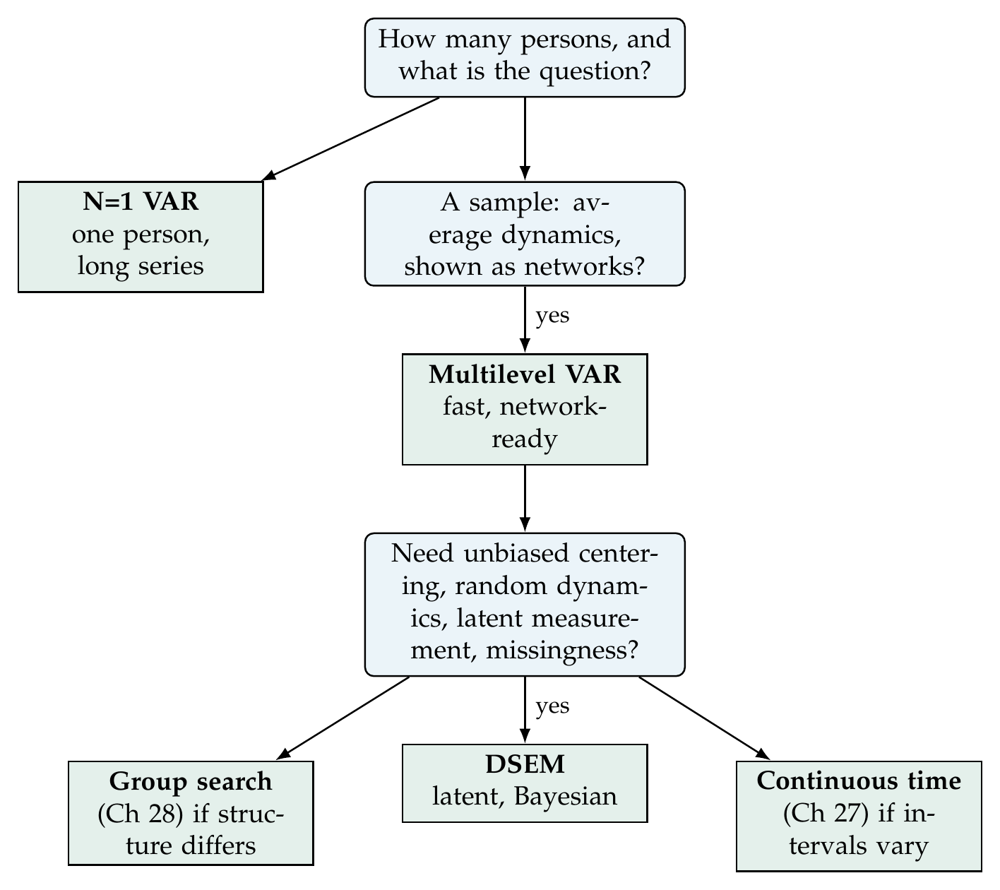
Note. The models form a graded family. One person with a long series calls for a VAR; a sample’s average dynamics call for multilevel VAR; latent centering, random dynamics, latent measurement, or missingness call for DSEM; badly unequal intervals call for continuous time (Chapter 27); qualitatively different structures across persons call for group search (Chapter 28).
Writing up a dynamic multilevel analysis extends the reporting discipline of the previous chapters with the decisions specific to these models. The report should state the model fit, VAR, multilevel VAR, or DSEM, and the centering used, because latent and sample-mean centering answer with different biases. It should give the estimated dynamics with their psychological reading, the average transition matrix as inertias and spillovers, and the heterogeneity as random-effect variances, with uncertainty. For DSEM it should report the estimator, the priors, the iterations, the convergence diagnostics, and the interval handling, and it should describe the sensitivity analyses run. Throughout it should keep the causal language calibrated to the design, reporting cross-lags as predictive within-person associations rather than as effects, and it should acknowledge the shrinkage of person-specific estimates and the series-length limits on what could be identified. A model paragraph reads: “A two-level DSEM was fit to negative affect and momentary stress (120 persons, up to 84 occasions each) in Mplus with the Bayesian estimator, latent person-mean centering, and random autoregressive and cross-lagged coefficients. The average within-person cross-lag from stress to next-moment negative affect was 0.24 (95% credible interval [.., ..]); it varied across persons (random-effect SD ..), and did not covary appreciably with mean stress level. Convergence was satisfactory (scale-reduction factor \(<1.05\); trace plots mixed), and the lag-1 conclusions were robust to a lag-2 specification. Cross-lags are interpreted as within-person predictive associations, not causal effects.”
Table 25.6. Reporting checklist for dynamic multilevel models.
| Element | What to report |
|---|---|
| Model and centering | VAR / multilevel VAR / DSEM; sample-mean vs latent centering |
| Design | Number of persons, occasions per person, interval structure, missingness |
| Dynamics | Average transition matrix (inertias, cross-lags) with uncertainty; psychological reading |
| Heterogeneity | Random-effect variances of the dynamics; covariances with person means |
| Innovations | Contemporaneous structure; random innovation variance if modeled |
| Estimation (DSEM) | Estimator, priors, iterations, scale-reduction factor, trace-plot check |
| Intervals | Interval handling (TINTERVAL grid or continuous-time model) |
| Sensitivity | Lag order, detrending variants, prior sensitivity |
| Interpretation | Cross-lags as prediction, not cause; shrinkage of person-specific estimates |
Note. The checklist extends the intensive-longitudinal reporting of Chapter 23 with the centering, random-dynamics, estimation, and interval decisions that are specific to the dynamic models, each of which changes what is being estimated.
Chapter Summary
The vector autoregression describes one person’s multivariate dynamics in a transition matrix whose diagonal is inertia and whose off-diagonal is cross-lagged transmission, whose eigenvalues govern stationarity and oscillation, and whose impulse response traces how a shock propagates, with Granger content that is predictive and interval-dependent rather than causal. Because the transition matrix differs across people, and because a single person’s series estimates it imprecisely, the multilevel VAR treats the person-specific matrices as random effects and recovers three distinct objects, the temporal, contemporaneous, and between-person matrices, which on affect_ema reproduce a known multilevel-VAR truth, the diagonal inertias sitting slightly low as the fingerprint of sample-mean bias. Joint estimation with shrinkage beats two-step pooling, lowering the error of person-specific estimates by pulling noisy fits toward the population. Dynamic structural equation modeling completes the architecture by decomposing each score into a latent person mean and a latent within-person process, which removes the sample-mean bias that afflicts short series, and by making the autoregressions, cross-lags, and log-innovation-variances random, distributions of dynamics with covariances that answer who has strong spillover and who is volatile, and by admitting a latent measurement layer that repairs the attenuation measurement error inflicts on autoregressions. Its estimation is Bayesian, its production standard is Mplus, and its convergence is read with the diagnostics of Chapter 17. The bias landscape, sample-mean centering, measurement error, two-step inflation, and interval coarseness, is a set of specific, directional errors each with a specific remedy, and the choice among VAR, multilevel VAR, DSEM, and the continuous-time and group-search models to come follows from the question, the data, and the machinery it justifies.
Asparouhov, T., Hamaker, E. L., & Muthén, B. (2018). Dynamic structural equation models. Structural Equation Modeling: A Multidisciplinary Journal, 25(3), 359–388. https://doi.org/10.1080/10705511.2017.1406803
Bringmann, L. F., Vissers, N., Wichers, M., Geschwind, N., Kuppens, P., Peeters, F., Borsboom, D., & Tuerlinckx, F. (2013). A network approach to psychopathology: New insights into clinical longitudinal data. PLoS ONE, 8(4), Article e60188. https://doi.org/10.1371/journal.pone.0060188
Bulteel, K., Mestdagh, M., Tuerlinckx, F., & Ceulemans, E. (2018). VAR(1) based models do not always outpredict AR(1) models in typical psychological applications. Psychological Methods, 23(4), 740–756. https://doi.org/10.1037/met0000178
Bulteel, K., Tuerlinckx, F., Brose, A., & Ceulemans, E. (2016). Clustering vector autoregressive models: Capturing qualitative differences in within-person dynamics. Frontiers in Psychology, 7, Article 1540. https://doi.org/10.3389/fpsyg.2016.01540
Epskamp, S. (2020). Psychometric network models from time-series and panel data. Psychometrika, 85(1), 206–231. https://doi.org/10.1007/s11336-020-09697-3
Epskamp, S., Waldorp, L. J., Mõttus, R., & Borsboom, D. (2018). The Gaussian graphical model in cross-sectional and time-series data. Multivariate Behavioral Research, 53(4), 453–480. https://doi.org/10.1080/00273171.2018.1454823
Gates, K. M., & Molenaar, P. C. M. (2012). Group search algorithm recovers effective connectivity maps for individuals in homogeneous and heterogeneous samples. NeuroImage, 63(1), 310–319. https://doi.org/10.1016/j.neuroimage.2012.06.026
Hamaker, E. L. (2012). Why researchers should think “within-person”: A paradigmatic rationale. In M. R. Mehl & T. S. Conner (Eds.), Handbook of research methods for studying daily life (pp. 43–61). Guilford Press.
Hamaker, E. L., Asparouhov, T., Brose, A., Schmiedek, F., & Muthén, B. (2018). At the frontiers of modeling intensive longitudinal data: Dynamic structural equation models for the affective measurements from the COGITO study. Multivariate Behavioral Research, 53(6), 820–841. https://doi.org/10.1080/00273171.2018.1446819
Hamaker, E. L., Dolan, C. V., & Molenaar, P. C. M. (2005). Statistical modeling of the individual: Rationale and application of multivariate stationary time series analysis. Multivariate Behavioral Research, 40(2), 207–233. https://doi.org/10.1207/s15327906mbr4002_3
Hamaker, E. L., & Muthén, B. (2020). The fixed versus random effects debate and how it relates to centering in multilevel modeling. Psychological Methods, 25(3), 365–379. https://doi.org/10.1037/met0000239
Jongerling, J., Laurenceau, J.-P., & Hamaker, E. L. (2015). A multilevel AR(1) model: Allowing for inter-individual differences in trait-scores, inertia, and innovation variance. Multivariate Behavioral Research, 50(3), 334–349. https://doi.org/10.1080/00273171.2014.1003772
Krone, T., Albers, C. J., & Timmerman, M. E. (2017). A comparative simulation study of AR(1) estimators in short time series. Quality & Quantity, 51(1), 1–21. https://doi.org/10.1007/s11135-015-0290-1
Lüdtke, O., Marsh, H. W., Robitzsch, A., Trautwein, U., Asparouhov, T., & Muthén, B. (2008). The multilevel latent covariate model: A new, more reliable approach to group-level effects in contextual studies. Psychological Methods, 13(3), 203–229. https://doi.org/10.1037/a0012869
McNeish, D., & Hamaker, E. L. (2020). A primer on two-level dynamic structural equation models for intensive longitudinal data in Mplus. Psychological Methods, 25(5), 610–635. https://doi.org/10.1037/met0000250
Molenaar, P. C. M. (1985). A dynamic factor model for the analysis of multivariate time series. Psychometrika, 50(2), 181–202. https://doi.org/10.1007/BF02294246
Nickell, S. (1981). Biases in dynamic models with fixed effects. Econometrica, 49(6), 1417–1426. https://doi.org/10.2307/1911408
Haslbeck, J. M. B., Bringmann, L. F., & Waldorp, L. J. (2021). A tutorial on estimating time-varying vector autoregressive models. Multivariate Behavioral Research, 56(1), 120–149. https://doi.org/10.1080/00273171.2020.1743630
Schuurman, N. K., Ferrer, E., de Boer-Sonnenschein, M., & Hamaker, E. L. (2016). How to compare cross-lagged associations in a multilevel autoregressive model. Psychological Methods, 21(2), 206–221. https://doi.org/10.1037/met0000062
Schuurman, N. K., & Hamaker, E. L. (2019). Measurement error and person-specific reliability in multilevel autoregressive modeling. Psychological Methods, 24(1), 70–91. https://doi.org/10.1037/met0000188