Chapter 26
Dynamic Factor Analysis and State-Space Models
The previous chapters built a series of dynamic models, one for a single autoregressive series, one for a vector of them, one that added a latent decomposition and random dynamics, and each arrived with its own notation and its own estimator. This chapter shows that they are one model. The linear Gaussian state-space form has two equations, a state equation that lets a latent process evolve and an observation equation that measures it with error, and by choosing what the state contains and how the matrices are populated it becomes an autoregression, a moving average, a vector autoregression, a latent growth curve, or a dynamic factor model. The Kalman filter is its inferential engine, a single recursion that delivers the likelihood for estimation, the exact treatment of missing occasions promised since Chapter 24, and the residuals for diagnosis, all as by-products of the same forward pass. The unification is not the chapter’s only purpose. The state-space form draws the line, blurred in every previous chapter, between measurement error and process noise, between the noise in the assessment and the genuine shocks to the person’s state, and it shows that conflating them biases the dynamics, the central psychometric payoff. And the dynamic factor model, the state-space form with a latent factor that both evolves and is measured, is the repair of the P-technique whose flaw Chapter 24 flagged: a person-specific factor structure that finally carries its own serial dependence. The matrices are introduced gently, each with a psychological sentence, because the models are latent-variable models over time, the cousins of the structural equation models of Part V, not artifacts of control engineering.
Learning Objectives
After working through this chapter, you should be able to: (1) write the state-space form, its state and observation equations, and populate its matrices for an AR(1) with measurement error, a local linear trend, a VAR(1), and a dynamic factor model, the “one form, many models” competence; (2) explain the Kalman filter and smoother as a predict-update recursion, read the Kalman gain as a reliability weight in the shrinkage sense of Chapter 13, and distinguish filtered from smoothed estimates; (3) separate measurement error from process noise and show why conflating them attenuates the dynamics, extending the measurement-error line of Chapter 25; (4) specify a dynamic factor model, distinguish the process-factor and direct-autoregressive-score forms, and state its identification requirements; (5) fit single-person and multi-person dynamic factor models and interpret person-specific measurement and dynamics; (6) diagnose a state-space fit through its standardized innovations, checking whiteness, normality, and outliers; and (7) know when the state-space machinery is worth its overhead relative to the tools of Chapter 25.
26.1 One Form to Hold Them All
The state-space form is two equations. The observation equation, \(\mathbf{y}_t = \mathbf{Z}\,\boldsymbol{\alpha}_t + \boldsymbol{\varepsilon}_t\) with \(\boldsymbol{\varepsilon}_t \sim N(\mathbf{0}, \mathbf{H})\), says that what is measured at occasion \(t\) is a loading matrix \(\mathbf{Z}\) times a latent state \(\boldsymbol{\alpha}_t\), plus measurement error \(\boldsymbol{\varepsilon}_t\). The state equation, \(\boldsymbol{\alpha}_t = \mathbf{T}\,\boldsymbol{\alpha}_{t-1} + \boldsymbol{\eta}_t\) with \(\boldsymbol{\eta}_t \sim N(\mathbf{0}, \mathbf{Q})\), says that the latent state evolves according to a transition matrix \(\mathbf{T}\), driven by process noise \(\boldsymbol{\eta}_t\). The two noise terms are not the same thing, and keeping them apart is the whole point. The measurement error \(\boldsymbol{\varepsilon}_t\) is assessment noise, the unreliability of the instrument, the part of a mood rating that reflects the vagueness of the item rather than the person’s actual state. The process noise \(\boldsymbol{\eta}_t\) is the genuine shock, the true change in the person’s state from one occasion to the next. Every previous chapter that regressed an observed score on its own lag silently fused these two, and this chapter separates them. Figure 26.1 draws the two equations with their psychological glosses.
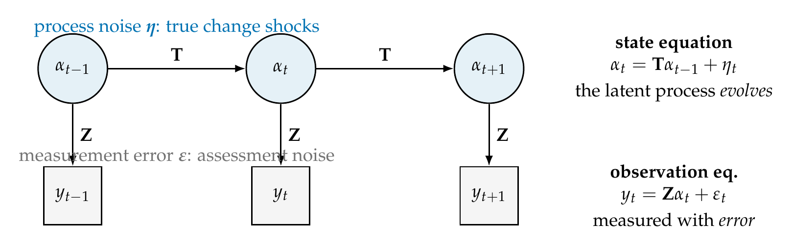
Note. The state equation lets a latent state \(\alpha_t\) evolve through a transition matrix \(\mathbf{T}\), disturbed by process noise (true change). The observation equation measures the state through a loading matrix \(\mathbf{Z}\), corrupted by measurement error (assessment noise). Separating the two noises is the form’s central psychometric contribution. The diagram is reused in Chapters 27 and 32.
The immediate payoff of the separation is a fact that reframes Chapter 24. An autoregression of order one observed with measurement error is not an autoregression at all; algebraically it is an ARMA(1,1), and its naive lag-one autocorrelation understates the true carryover in proportion to the unreliability of the measure. The mechanism is exactly the attenuation that measurement error inflicts on any correlation, applied here to the correlation of a series with its own past. Figure 26.2 makes this concrete on kalman_n1, a single-subject series generated from a latent AR(1) with true carryover \(0.60\) observed with error at a reliability of \(0.65\). The left panel shows the naive autoregression falling steadily as reliability worsens, reaching well below the true value; on this series the naive lag-one autocorrelation is \(0.46\), badly short of the generating \(0.60\). The right panel shows the repair and its cost together: a Kalman-based maximum-likelihood fit that models the measurement error separately recovers a carryover of \(0.61\), and across a hundred simulated series it is unbiased on average, but its per-series estimate is noisy, because separating two variances from one short series is a demanding request. The separation succeeds in expectation and must be reported with its uncertainty.
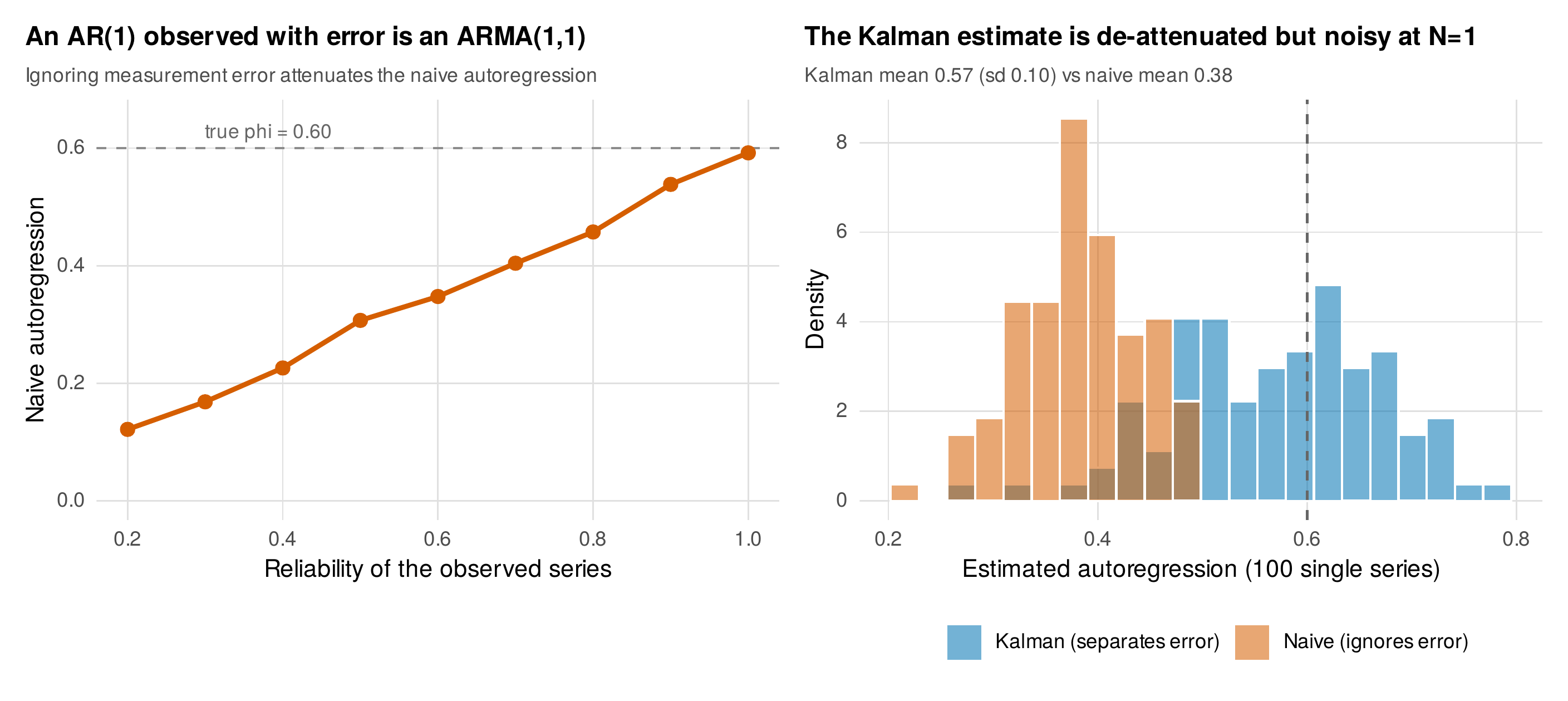
Note. Left: the naive autoregression of an error-laden series falls below the true carryover (\(0.60\)) as reliability worsens. Right: sampling distributions across 100 single series; the Kalman estimate that models measurement error separately is centered near the truth while the naive estimate is attenuated toward zero. The separation is unbiased on average but imprecise from one series.
The same two equations, with different matrices, become the familiar models, and filling those matrices is the competence this section builds. Figure 26.3 shows five cards. An AR(1) with measurement error has a scalar state, \(\mathbf{T} = \phi\), \(\mathbf{Z} = 1\), process variance \(\mathbf{Q} = \sigma^2_\eta\), and measurement variance \(\mathbf{H} = \sigma^2_\varepsilon\). A local linear trend, the structural time-series model of a level that drifts with a slowly changing slope, has a two-dimensional state of level and slope with a transition matrix that carries the slope into the level. A VAR(1) has a vector state and a full transition matrix, the model of Chapter 25 with \(\mathbf{H} = \mathbf{0}\) when measured without error or \(\mathbf{H} \neq \mathbf{0}\) when not. A dynamic factor model has a latent factor state that evolves and a loading matrix that measures it through several indicators. And the latent growth curve of Chapter 19 is a state-space model with a state of intercept and slope, a transition matrix that holds them constant, and a time-varying loading matrix that reads the slope onto successive occasions, which unifies Parts V and VI under one form. Table 26.1 names each matrix with its dimension, its psychological meaning, and its structural-equation or multilevel analogue, and Table 26.2 states what each of the five models puts in each matrix.
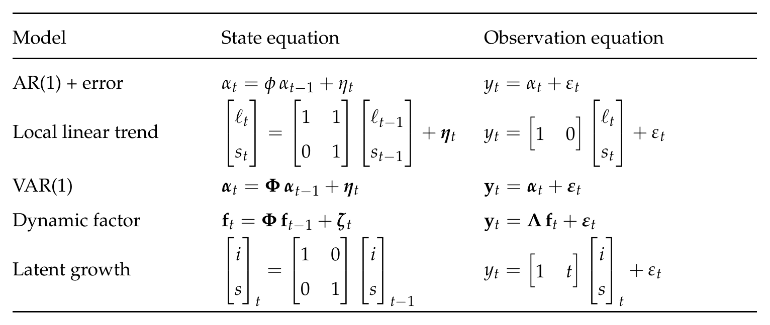
Note. Each familiar model is the state-space form with particular matrices. The autoregression, the trend model, the vector autoregression, the dynamic factor model, and the latent growth curve differ only in what the state contains, how the transition matrix moves it, and how the loading matrix reads it. The latent growth loading is time-varying, which is how a static growth model becomes a state-space model.
Table 26.1. State-space objects and their analogues.
| Object | Name | Psychological meaning | SEM/MLM analogue |
|---|---|---|---|
| \(\boldsymbol{\alpha}_t\) | State vector | The person’s latent state now | Latent factor / random effect |
| \(\mathbf{T}\) | Transition matrix | How the state carries and couples forward | Autoregression / cross-lag |
| \(\mathbf{Q}\) | Process covariance | Size of true change shocks | Innovation / disturbance variance |
| \(\mathbf{Z}\) | Loading matrix | How the state shows in the measures | Factor loadings |
| \(\mathbf{H}\) | Measurement covariance | Assessment noise | Residual / unique variance |
| \(\boldsymbol{\alpha}_1, \mathbf{P}_1\) | Initial state | Where the process starts | Exogenous mean/variance |
Note. Every state-space object has a familiar cousin. The transition matrix is the autoregression, the loading matrix is the factor loadings, the process covariance is the innovation variance, and the measurement covariance is the unique variance of a measurement model.
Table 26.2. What each model puts in each matrix.
| Model | State dim | \(\mathbf{T}\) | \(\mathbf{Z}\) | \(\mathbf{H}\) |
|---|---|---|---|---|
| AR(1) + error | 1 | \(\phi\) | \(1\) | \(\sigma^2_\varepsilon > 0\) |
| Local linear trend | 2 | \(\left[\begin{smallmatrix}1&1\\0&1\end{smallmatrix}\right]\) | \([1\ 0]\) | \(\sigma^2_\varepsilon\) |
| VAR(1) | \(p\) | \(\boldsymbol{\Phi}\) (full) | \(\mathbf{I}\) | \(\mathbf{0}\) or diag |
| Dynamic factor | \(k\) (factors) | \(\boldsymbol{\Phi}\) (factor VAR) | \(\boldsymbol{\Lambda}\) (loadings) | diag \(> 0\) |
| Latent growth | 2 | \(\mathbf{I}\) | \([1\ \ t]\) (time-varying) | \(\sigma^2_\varepsilon\) |
Note. The models differ in state dimension and in which matrices are free, fixed, or time-varying. Fixing \(\mathbf{H}=\mathbf{0}\) turns a state-space model into an observed-score model, the simplification the chapter warns against when measurement error is real.
26.2 The Kalman Engine
The Kalman filter is a single recursion that walks forward through the series, and at each occasion it does two things. It predicts: given the best estimate of the state at the previous occasion, the transition matrix carries it forward to a prediction of the state now, and the uncertainty grows by the process noise. It updates: the new observation arrives, its discrepancy from what the prediction implied is the innovation, and the state estimate is corrected toward the observation by an amount called the Kalman gain. Figure 26.4 draws the loop. The gain is the heart of the matter and it is a reliability weight in exactly the sense of Chapter 13’s shrinkage. When the measurement is precise relative to the state uncertainty, the gain is large and the estimate moves most of the way to the observation; when the measurement is noisy, the gain is small and the estimate stays close to the model’s prediction. The filter is optimally trading a prior forecast against a noisy datum, precision against precision, which is the same weighted-average logic that shrinks a person’s estimate toward a group mean, now operating in time.
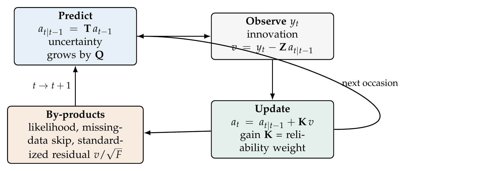
Note. At each occasion the filter predicts the state from the transition matrix (uncertainty growing by the process noise), then updates toward the new observation by the Kalman gain, a reliability weight that is large when the measurement is precise and small when it is noisy. The likelihood, the missing-data handling, and the standardized residuals fall out of the same pass.
Three things fall out of that single forward pass, and together they are why the state-space form is worth its machinery. The likelihood comes free through the prediction-error decomposition: each innovation, standardized by its own variance, contributes a Gaussian term, and their sum is the exact log-likelihood, so maximum-likelihood estimation of the transition, loading, and variance parameters is an optimization over repeated filter runs. Missing data are handled exactly and without imputation: when an occasion is unobserved, the update step is simply skipped, the prediction carries forward, and the state uncertainty grows until the next observation arrives, which is the principled repair of the naive interpolation that Chapter 24 showed inflates autocorrelation. And the standardized one-step-ahead innovations are the residuals for diagnosis, white and normal when the model is right. The foundations box states the likelihood decomposition and the AR-plus-error algebra formally.
Foundations Box • The prediction-error decomposition and the AR-plus-error algebra
Run the filter and collect, at each observed occasion, the innovation \(v_t = y_t - \mathbf{Z}\,a_{t|t-1}\) and its variance \(F_t = \mathbf{Z}\,P_{t|t-1}\mathbf{Z}^{\top} + \mathbf{H}\). Because the innovations are, by construction, mutually independent and Gaussian, the log-likelihood of the whole series factorizes into their contributions, \(\log L = -\tfrac{1}{2}\sum_t \big(\log 2\pi + \log F_t + v_t^2/F_t\big)\), the prediction-error decomposition. This is what makes maximum likelihood feasible for the entire state-space family from one recursion. For the AR-plus-error case, let the latent state be \(\alpha_t = \phi\,\alpha_{t-1} + \eta_t\) with \(\mathrm{Var}(\alpha) = \sigma^2_\eta/(1-\phi^2)\), observed as \(y_t = \alpha_t + \varepsilon_t\) with \(\mathrm{Var}(\varepsilon) = \sigma^2_\varepsilon\). The observed lag-one autocorrelation is \(\rho_1 = \phi\,\mathrm{Var}(\alpha)/(\mathrm{Var}(\alpha) + \sigma^2_\varepsilon) = \phi\,R\), where \(R\) is the reliability, and higher lags decay as \(\phi^k R\), the autocorrelation signature of an ARMA(1,1). The naive estimate returns \(\phi R\), attenuated by exactly the reliability, and only a model that carries \(\sigma^2_\varepsilon\) as a separate parameter recovers \(\phi\) itself.
The Kalman arc on kalman_n1 demonstrates the separation. Fitting the AR-plus-error model by maximizing the filter likelihood recovers a carryover of \(0.61\) against the generating \(0.60\), and the smoother then produces the best retrospective estimate of the latent state at each occasion. Figure 26.5 shows the filtered and smoothed latent paths with their uncertainty ribbons beneath the noisy observations. The filtered estimate uses only the past and is available in real time; the smoothed estimate uses the whole series and is tighter and closer to the true latent state, the retrospective best guess. The choice between them is a choice of estimand, set out in Table 26.3: filtering is for monitoring as data arrive, the clinical use that Chapter 33 develops for just-in-time interventions, while smoothing is for the historical reconstruction that a completed study wants.
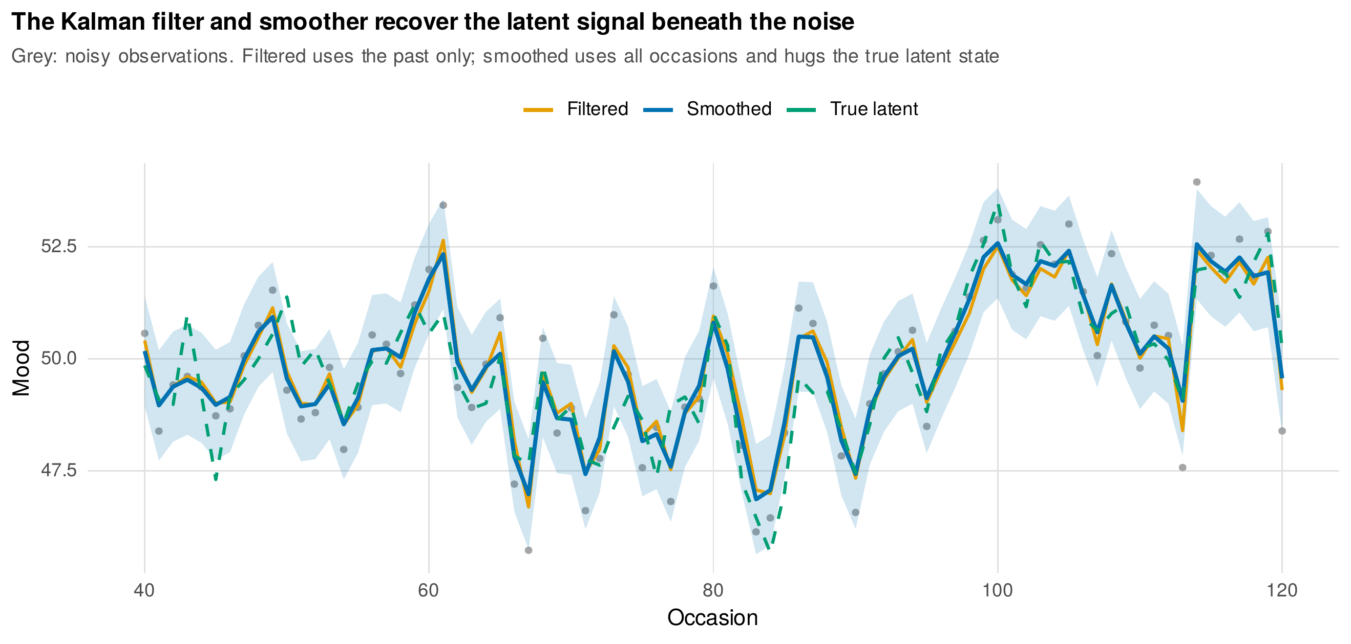
Note. The filtered (past only) and smoothed (whole series) estimates of the latent state on kalman_n1, with the smoothed uncertainty ribbon, against the noisy observations and the true latent path. Both recover the signal beneath the assessment noise; the smoother is tighter and tracks the truth more closely.
Table 26.3. Filtering versus smoothing.
| Filtering | Smoothing | |
|---|---|---|
| Uses | Observations up to \(t\) only | All observations in the series |
| Estimand | State now, given the past | State at \(t\), given everything |
| Uncertainty | Wider | Tighter |
| Availability | Real time, as data arrive | Retrospective, after the study |
| Use case | Monitoring, forecasting, JITAI (Ch 33) | Historical reconstruction, analysis |
Note. The two estimates answer different questions. Filtering is causal in time and suited to real-time monitoring; smoothing conditions on the whole series and is the right choice for after-the-fact analysis of a completed study.
The missing-data repair is the payoff Chapter 24 promised. Masking a stretch of kalman_n1 and running the filter, the state estimate through the gap is not a straight line but a curve that reverts toward the process mean while its uncertainty ribbon widens to reflect the absence of data, and closes again when observations resume. Figure 26.6 contrasts this with linear interpolation, which draws a confident straight line through the gap and thereby claims a certainty it does not have. The consequences are measurable: the Kalman smoother reconstructs the latent trajectory in the gap with a root-mean-square error of \(1.43\) against the true latent state, while interpolation manages only \(2.04\), and the carryover estimated on the gapped series by the Kalman method, \(0.57\), stays close to the full-data value, whereas interpolating and then estimating naively inflates the observed autocorrelation. The filter treats a missing occasion as what it is, an absence of information, rather than as a value to invent. The run-it-in-R panel carries the whole arc.
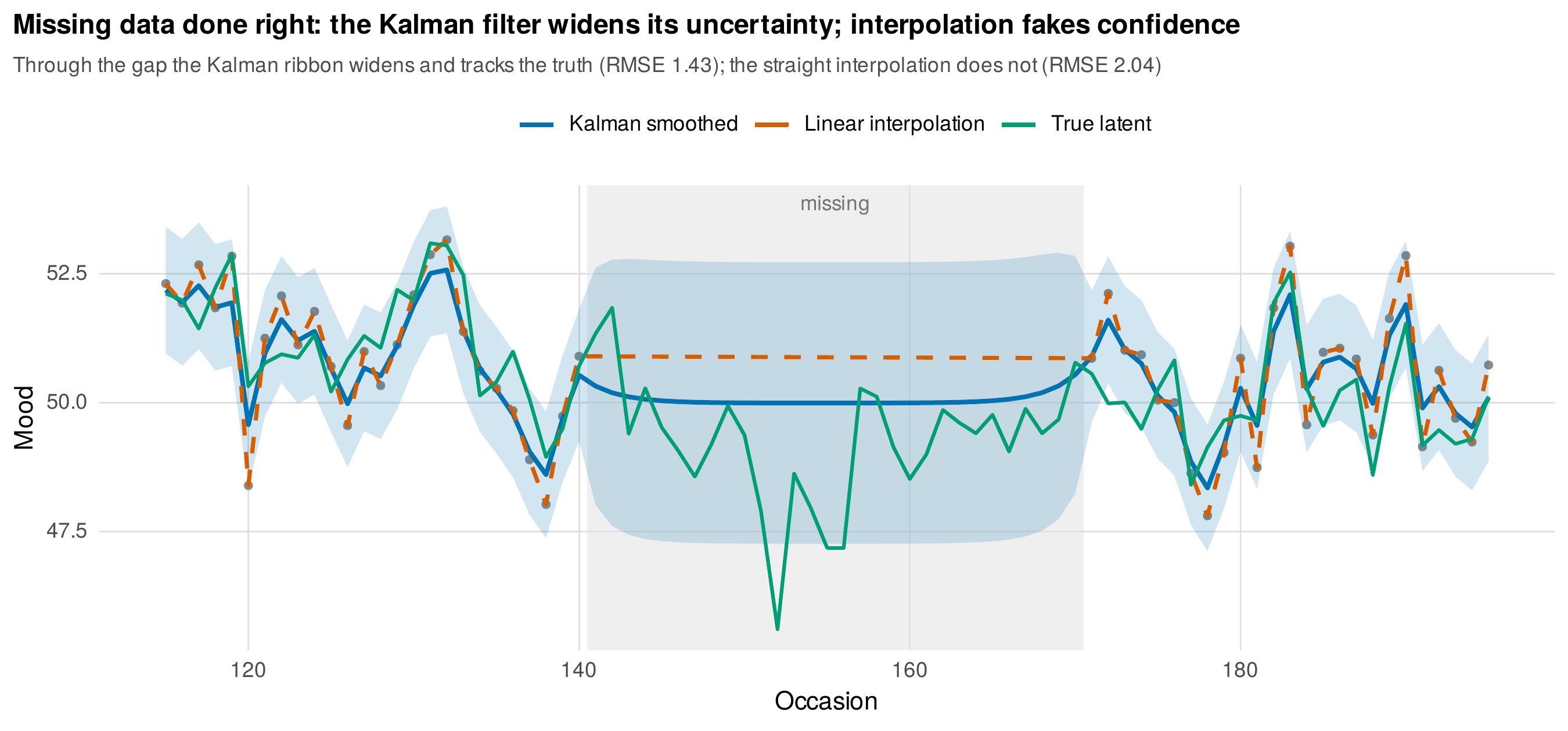
Note. Through a masked stretch of kalman_n1, the Kalman smoother’s uncertainty ribbon widens and its estimate reverts toward the mean, tracking the true latent state (RMSE \(1.43\)); linear interpolation draws a confident straight line that does not (RMSE \(2.04\)). The filter represents missingness as absence of information, not as an invented value.
# The Kalman arc on kalman_n1: separate measurement error from process noise
d <- readRDS("Examples/data/kalman_n1.rds")            # y (observed), eta_true (latent)
yc <- d$y - mean(d$y)
# maximize the filter likelihood over (phi, process var q, measurement var r)
negll <- function(par) {                               # kalman_filter() hand-rolled in ch26_analysis
  phi <- tanh(par[1]); q <- exp(par[2]); r <- exp(par[3])
  -kalman_filter(matrix(yc), matrix(phi), matrix(1), matrix(q), matrix(r),
                 a1 = 0, P1 = matrix(q/(1-phi^2)))$loglik
}
fit <- optim(c(atanh(.3), 0, 0), negll, method = "BFGS")
tanh(fit$par[1])                                       # phi ~ 0.61 (naive lag-1 autocorr = 0.46)
# smoothed latent state + widening uncertainty across a masked gap:
kf <- kalman_filter(matrix(d$y_gap - mean(d$y_gap, na.rm=TRUE)), ...)  # NA occasions skipped
ks <- kalman_smoother(kf, matrix(tanh(fit$par[1])))
26.3 Dynamic Factor Models
The dynamic factor model is the state-space form with a latent factor for its state, and it is the repair of the P-technique that Chapter 24 left broken. P-technique factor-analyzed one person’s items across occasions but treated the occasions as independent, discarding the serial dependence that is the point of a time series. The dynamic factor model keeps the factor structure, a small number of latent factors that load onto the observed items, and adds dynamics, letting the factors evolve as a vector autoregression, so that the latent process both is measured, through the loading matrix, and carries itself forward, through the transition matrix. The result is a person-specific measurement model with person-specific dynamics, idiographic measurement realized. Two canonical forms exist and the distinction is worth stating, as Figure 26.7 draws it. In the process-factor form, the tradition of Molenaar, the latent factor follows the autoregression and the measurement is contemporaneous and clean, so the dynamics live entirely in the factor. In the direct-autoregressive form, the autoregression is written on the factor scores with lagged loadings, distributing the memory across the measurement. The forms can be made equivalent under conditions, and Table 26.4 states when each is preferred and what each requires for identification.
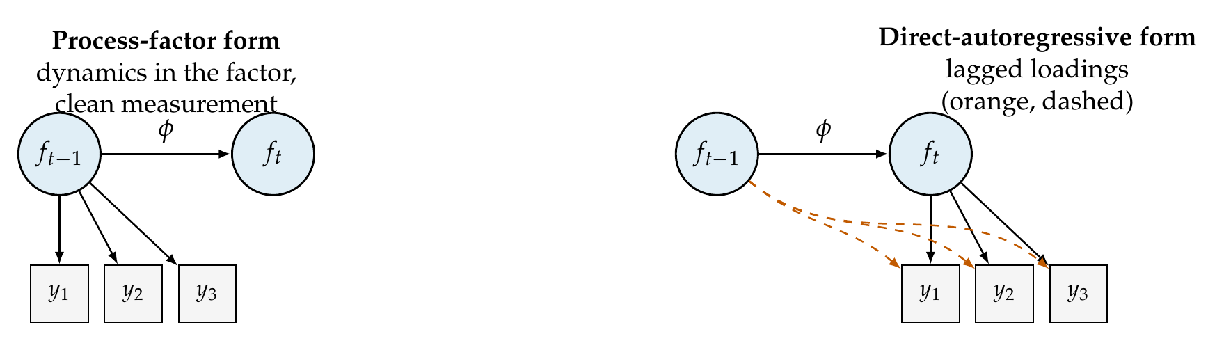
Note. Process-factor form (left): the latent factor follows the autoregression and the loadings measure the current factor cleanly, so all dynamics reside in the factor. Direct-autoregressive form (right): the memory is carried by lagged loadings from earlier factor scores onto current indicators. The forms coincide under conditions; the process-factor form is the more common in psychology.
Table 26.4. Dynamic factor model variants.
| Form | Structure | Identification and use |
|---|---|---|
| Process-factor (white-noise) | Factor follows VAR; contemporaneous clean loadings | Scale set by an anchor loading or unit factor variance; preferred when dynamics are a factor property |
| Direct-autoregressive score | Autoregression on scores; lagged loadings | Lag structure must be constrained; useful when memory is measurement-carried |
| Multi-factor | Several factors with a factor VAR | Needs enough indicators per factor and enough occasions; cross-lags identify with care |
Note. Identification requires setting the factor scale (an anchor loading fixed to one, or the factor variance fixed) and a defensible lag structure. With few occasions, a rich multi-factor model is not identifiable; simplify or pool across persons.
That the model recovers a known structure is shown on dfm_sim, a two-factor series with a known loading matrix and a known factor transition, fit here by a hand-written expectation-maximization algorithm whose expectation step is the Kalman smoother and whose maximization step updates the loadings, the transition, and the variances in closed form. Figure 26.8 shows the recovery: the loadings return close to their generating values, the factor transition recovers the autoregressive diagonal and the cross-lag from the second factor into the first, and the smoothed factor scores correlate with the true factors at \(0.94\) and \(0.91\). The estimator reconstructs a latent dynamic structure from noisy multivariate indicators, the validation that licenses its use where truth is unknown.
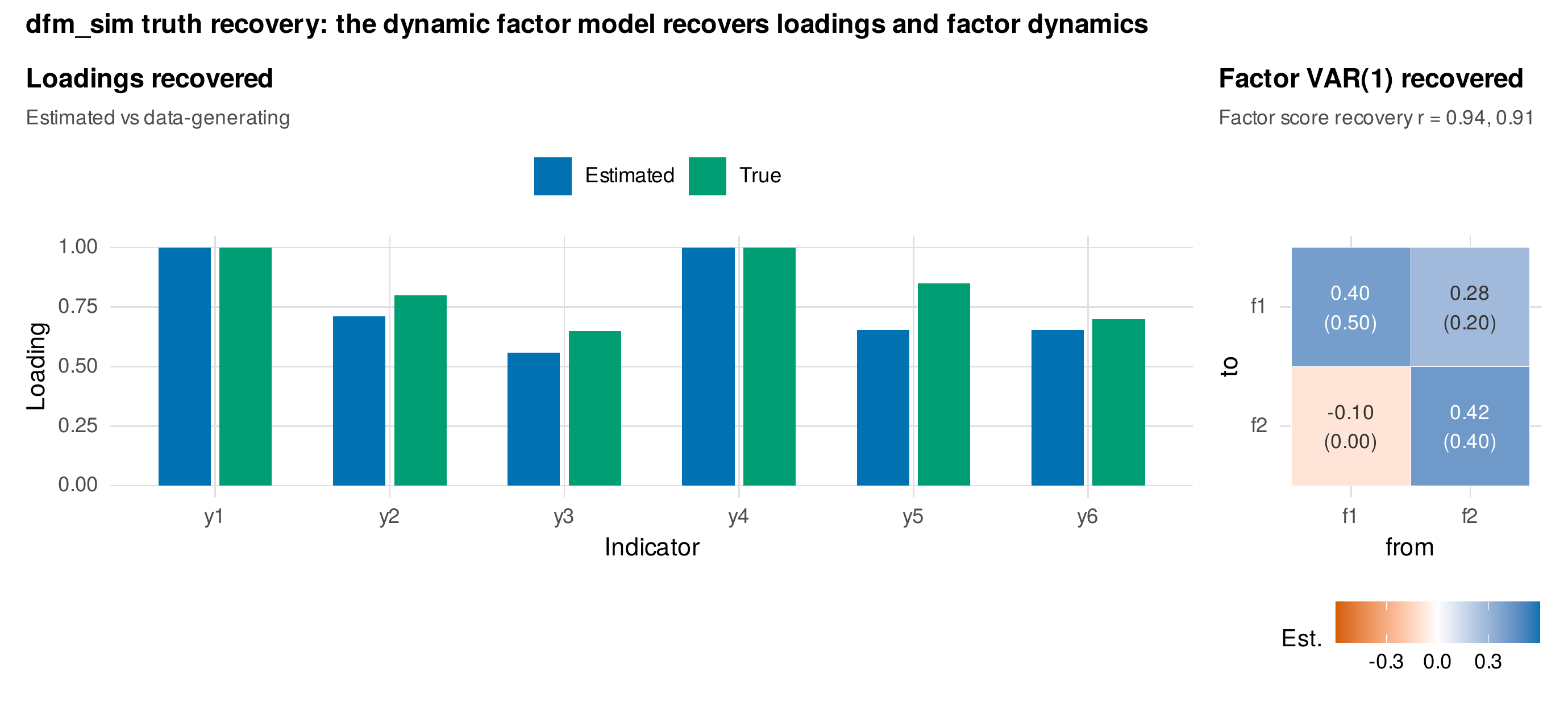
dfm_sim.Note. Estimated versus generating loadings (left) and factor transition matrix (right, estimated with the true value in parentheses) for a two-factor dynamic factor model fit to dfm_sim by Kalman-EM. The loadings and the factor VAR are recovered, and the smoothed factor scores correlate with the true factors at \(0.94\) and \(0.91\).
The idiographic promise is realized on real items. Fitting a one-factor dynamic factor model to the four negative-affect items of two affect_ema persons, with the factor free to follow its own autoregression, returns two genuinely different pictures, shown in Figure 26.9. For the first person the negative-affect factor is coherent and persistent: all four items relate substantially to it, feeling nervous most strongly, and the factor carries a moderate inertia of \(0.41\), so their negative affect lingers. For the second person the factor has almost no carryover, an inertia of \(0.06\), and a different indicator profile: feeling tense is its strongest sign while feeling nervous is nearly unrelated to it. The same four items assemble into different personal structures with different dynamics, which is the nonergodicity of Chapter 24 made concrete at the level of measurement itself, and it is precisely what a single between-person factor analysis, imposing one loading pattern and no dynamics on everyone, cannot represent. Multi-person strategies follow two routes: the replicated single-subject approach fits each person separately and summarizes the distribution of their structures and dynamics, while the state-of-the-art multilevel dynamic factor model pools them, which is the measurement layer of the DSEM of Chapter 25, the same idea reached from the factor-analytic side.
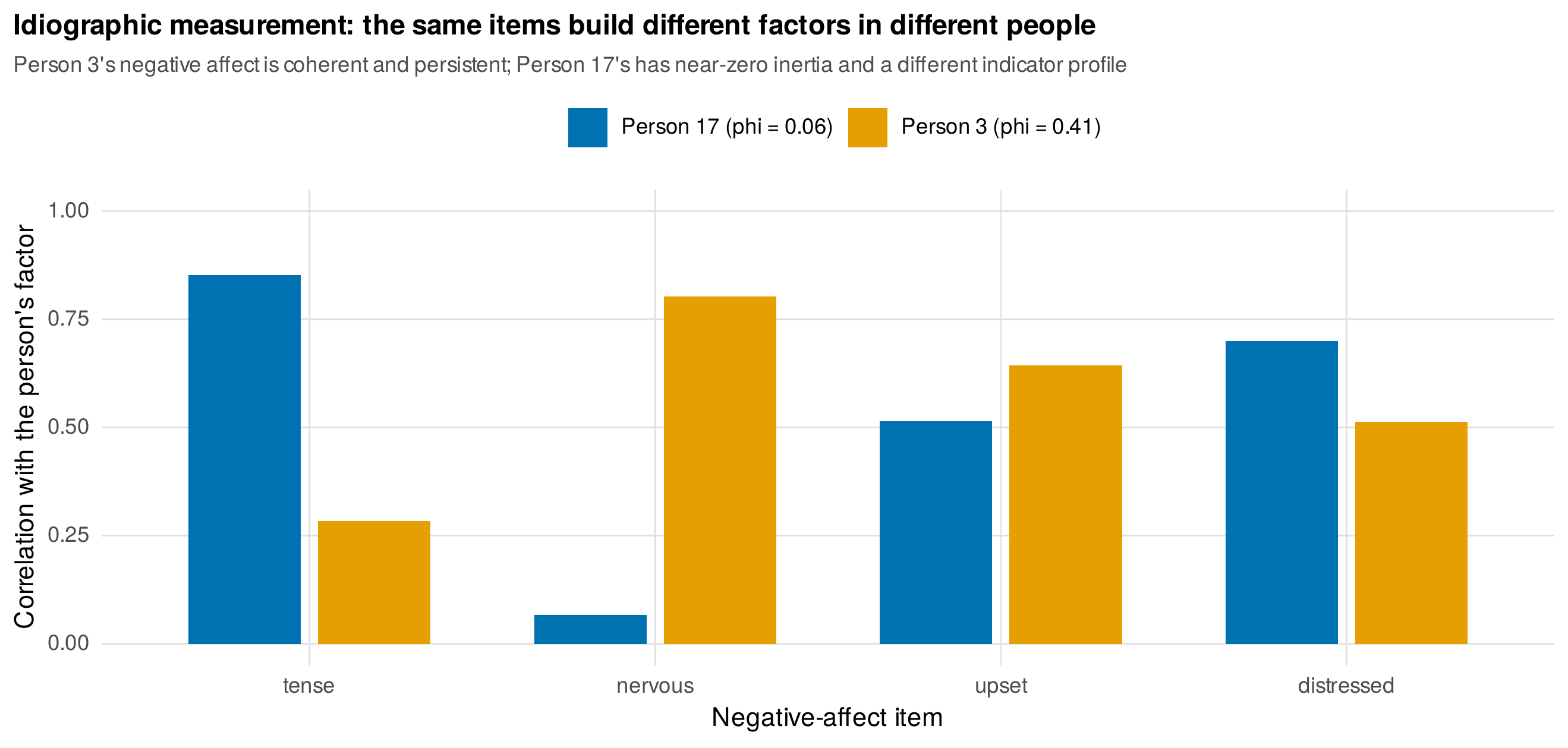
Note. One-factor dynamic factor models of four negative-affect items for two affect_ema persons, showing each item’s correlation with the person’s factor. Person 3’s factor is coherent and persistent (inertia \(0.41\)); Person 17’s has near-zero inertia (\(0.06\)) and a different indicator profile. Person-specific measurement and dynamics, which a single between-person model cannot capture.
26.4 Diagnostics and Selection
A fitted state-space model is judged, like any time-series model, by whether it has left white noise behind, and the object of scrutiny is the standardized one-step-ahead innovation, the filter’s residual divided by its own predicted standard deviation. If the model is correctly specified these standardized innovations are independent and standard normal, so three checks apply. Their autocorrelation should be negligible, confirmed by eye and by a Ljung-Box test, because remaining serial structure means the dynamics are misspecified. Their distribution should be normal, checked by a quantile plot and a normality test, because heavy tails signal outliers or a non-Gaussian process. And individual large values flag outliers, which in a psychological series are often not nuisances to be trimmed but substantive events, a stressor, a crisis, a change of regime, to be understood rather than discarded, the pointer to Chapter 32. Figure 26.10 shows the panel for the AR-plus-error fit on kalman_n1: the standardized innovations scatter within their bands, their autocorrelation is negligible with a Ljung-Box \(p\) of \(0.93\), and their quantile plot is straight with a normality \(p\) of \(0.23\), so the model has whitened the series and is retained.
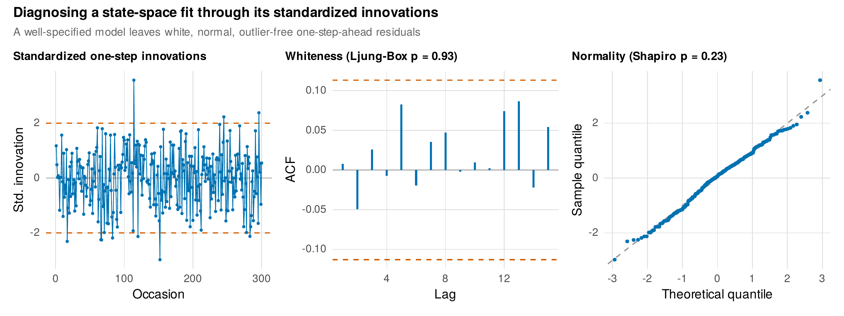
Note. Standardized one-step-ahead innovations from the AR-plus-error fit on kalman_n1: their series within \(\pm 2\) bands (left), their autocorrelation with the Ljung-Box result (center), and their normal quantile plot (right). White, normal, outlier-free residuals indicate an adequate model.
Selection among specifications follows the parsimony doctrine that this book has urged throughout, sharpened by the reality of psychological series lengths. Nested models, an AR-plus-error against a plain AR, or a one-factor against a two-factor dynamic model, are compared by a likelihood-ratio test using the prediction-error likelihood; non-nested ones by an information criterion. The temptation to enrich the state, to add a second factor, a higher lag, a time-varying parameter, must be resisted at the series lengths psychology collects, because a state-space model with more parameters than the data can identify will converge to a boundary, report a variance component pinned at zero, or fit the sample and fail to replicate, the same Heywood-case and over-parameterization hazards that Chapter 13 raised for variance components. The pitfalls box collects the specific ways these models mislead.
Common Pitfall • Four ways a state-space analysis misleads
First, fixing the measurement error to zero for simplicity, which is the chapter’s own central hook violated: an observed-score dynamic model attributes assessment noise to the process and attenuates every autoregression, so measurement error should be modeled, not assumed away, whenever the measure is fallible. Second, over-specifying the state at psychological length, adding factors, lags, or time-varying parameters that a series of a hundred occasions cannot identify, producing boundary estimates and non-replicable fits. Third, interpreting the filtered or smoothed states as if they were observed data, forgetting that they are posterior estimates with uncertainty, so that a plot of smoothed states without their ribbons overstates what is known and a downstream analysis that treats them as data understates its own uncertainty. Fourth, reporting a smoothed state estimate as the person’s true score, when it is a model-dependent posterior that would shift under a different specification of the dynamics or the measurement.
26.5 Software and When the Machinery Pays
The state-space form is served by several R packages whose strengths differ, and Figure 26.11 and Table 26.5 lay out the landscape. The KFAS package is fast and exact for linear Gaussian models and their exponential-family extensions, the workhorse for the filtering and smoothing of this chapter. The MARSS package specializes in multivariate autoregressive state-space models with an accessible interface for ecological and psychological time series. The dynr package, whose model-cooking conventions recur in Chapter 32, adds regime-switching and nonlinear dynamics, the readiness for the change-point and oscillator models to come. And OpenMx defines state-space models in a structural-equation environment with definition variables, the natural home for readers fluent in SEM. Mplus, through its dynamic structural equation modeling, is the adjacent production tool whose distinctive addition is multilevel pooling across persons; the distinction worth holding is that DSEM adds the multilevel layer while the state-space packages add structural freedom, the ability to specify custom transition and measurement structures that a fixed DSEM template does not expose. None of these packages was used for the analyses here, which were built from a hand-written filter, smoother, and EM algorithm so that every object could be checked against a known truth; readers with production needs should reach for the packages, and readers who want to understand what the packages do will find the mechanisms in the shipped scripts.
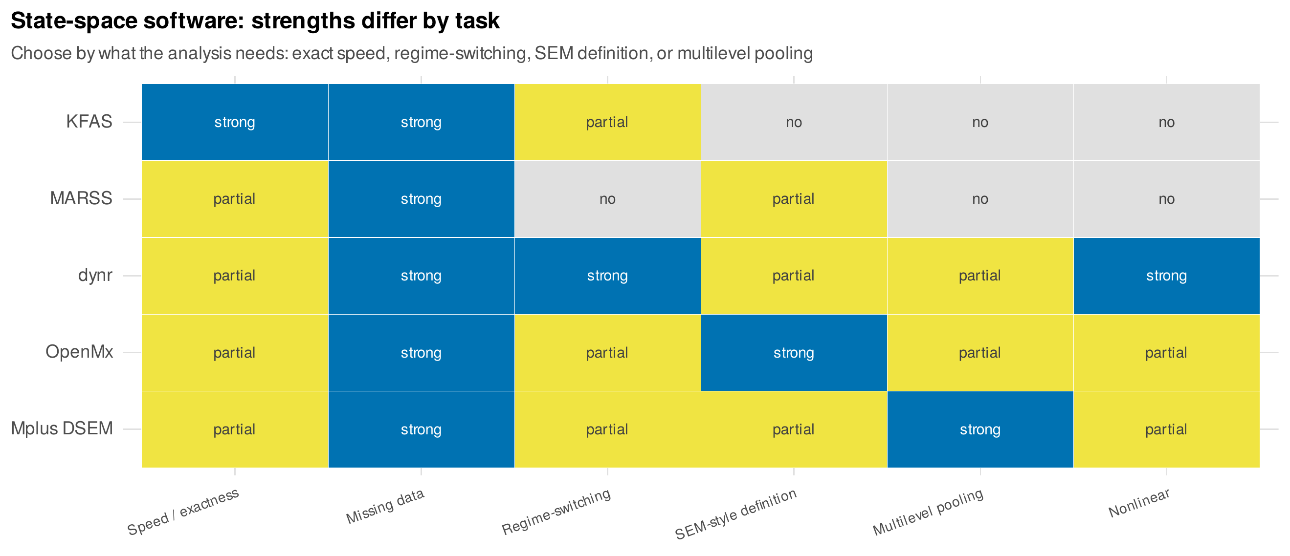
Note. A capability matrix for the main state-space tools. Strengths differ: KFAS for exact speed, dynr for regime-switching and nonlinearity, OpenMx for SEM-style definition, and Mplus DSEM for multilevel pooling. The choice follows what the analysis needs.
Table 26.5. State-space software feature comparison.
| Tool | Strength | Watch for | Best when |
|---|---|---|---|
| KFAS | Fast, exact linear Gaussian | Linear/Gaussian only | Filtering, smoothing, ML on a fixed model |
| MARSS | Accessible MARSS interface | Larger models slow | Multivariate AR state-space, teaching |
| dynr | Regime-switching, nonlinear | Steeper setup | Change-points (Ch 32), nonlinear dynamics |
| OpenMx | SEM-native, definition vars | Verbose specs | SEM-fluent readers; custom structures |
| Mplus DSEM | Multilevel pooling | Fixed template | Many persons, random dynamics (Ch 25) |
Note. The state-space packages add structural freedom; Mplus DSEM adds multilevel pooling. Choose by whether the analysis most needs exactness, regime-switching, SEM definition, or pooling across persons.
When the state-space machinery earns its overhead is the practical question, and the answer is specific. It pays when measurement error must be separated from process noise, because no observed-score model can do that; when data are missing and the missingness must be handled exactly rather than imputed; when the target is a latent multivariate process, a dynamic factor structure that no single-indicator model reaches; and when the structure is custom, a transition or measurement matrix that a packaged model does not offer. It does not pay when a multilevel VAR of Chapter 25 answers the question with less assembly and the measurement error is negligible, in which case the simpler tool is the honest choice. The continuous-time models of the next chapter are the same state-space architecture with the transition governed by a differential equation rather than a discrete step, which is how the form accommodates the unequal intervals that Chapter 25 flagged, and the regime-switching models of Chapter 32 let the transition matrix itself change, which is how the form accommodates the change points this chapter’s outliers hinted at.
In Practice • Numerical hygiene and runtime for state-space fits
Initialize with care: when the initial state is genuinely unknown, use a diffuse prior, a large initial variance that lets the data speak, rather than a tight guess that biases the early estimates. Scale the variables to comparable ranges before fitting, because the optimizer and the matrix inversions behave badly when variances differ by orders of magnitude. Parameterize variances on the log scale and autoregressions through a bounded transform so the optimizer cannot wander into negative variances or explosive dynamics. Expect the expectation-maximization algorithm to be reliable but slow to its last digits, and direct maximum likelihood to be faster but more sensitive to starting values, so run from several starts and confirm the likelihood agrees. And confirm convergence by inspecting the standardized innovations, not merely by the optimizer’s report of success, because a converged optimizer on a misspecified model is still a misspecified model.
Writing up a state-space or dynamic factor analysis extends the reporting of the previous chapters with the decisions specific to the form. The report should state the state-space model fit, what the state contains and how the transition and measurement matrices are specified, and in particular whether measurement error was modeled or fixed to zero, because that single choice governs whether the dynamics are attenuated. It should give the estimated dynamics with their psychological reading and their uncertainty, report how missing data were handled, and present the convergence and residual diagnostics, the standardized-innovation checks, that certify the fit. For a dynamic factor model it should state the identification, the anchor or scale constraint and the lag structure, and for an idiographic analysis it should be explicit that the structure and dynamics are person-specific and not assumed to generalize. A model sentence reads: “A one-factor dynamic factor model with a latent AR(1) factor and freely estimated measurement-error variances was fit to the four negative-affect items by Kalman-EM; the factor’s inertia was \(0.41\) for Person 3 and \(0.06\) for Person 17, and the two persons’ loading profiles differed, indicating person-specific measurement and dynamics; standardized innovations were white and approximately normal.”
Chapter Summary
The linear Gaussian state-space form is the mother model of this part: a state equation that lets a latent process evolve through a transition matrix, disturbed by process noise, and an observation equation that measures the state through a loading matrix, corrupted by measurement error. Populating the matrices yields the autoregression, the trend model, the vector autoregression, the latent growth curve, and the dynamic factor model as special cases, one form holding them all. The Kalman filter is its engine, a predict-update recursion whose gain is a reliability weight in the shrinkage sense, and from a single forward pass fall the likelihood by the prediction-error decomposition, the exact handling of missing occasions by skipped updates, and the standardized innovations for diagnosis. The form’s central psychometric contribution is to separate measurement error from process noise: an autoregression observed with error is an ARMA(1,1) whose naive estimate is attenuated by the reliability, and only a model that carries the measurement variance separately recovers the true carryover, which on kalman_n1 it does, though a single short series estimates the split with real imprecision. The missing-data repair promised in Chapter 24 is delivered, the filter widening its uncertainty through a gap and reconstructing the latent trajectory more accurately than the interpolation that fakes confidence. The dynamic factor model repairs P-technique by giving a person-specific factor structure its own dynamics, recovers a known loading matrix and factor transition on dfm_sim, and reveals on real items that two people build different factors from the same measures with different inertias, idiographic measurement realized. A fit is judged by the whiteness and normality of its innovations and chosen with the parsimony that psychological series lengths demand, and the machinery is worth its overhead exactly when measurement error, missing data, latent multivariate dynamics, or custom structure make the simpler tools of Chapter 25 insufficient.
Browne, M. W., & Nesselroade, J. R. (2005). Representing psychological processes with dynamic factor models: Some promising uses and extensions of ARMA time series models. In A. Maydeu-Olivares & J. J. McArdle (Eds.), Contemporary psychometrics: A festschrift for Roderick P. McDonald (pp. 415–452). Lawrence Erlbaum Associates.
Chow, S.-M., Ferrer, E., & Nesselroade, J. R. (2007). An unscented Kalman filter approach to the estimation of nonlinear dynamical systems models. Multivariate Behavioral Research, 42(2), 283–321. https://doi.org/10.1080/00273170701360423
Chow, S.-M., Ho, M.-H. R., Hamaker, E. L., & Dolan, C. V. (2010). Equivalence and differences between structural equation modeling and state-space modeling techniques. Structural Equation Modeling: A Multidisciplinary Journal, 17(2), 303–332. https://doi.org/10.1080/10705511003661553
Durbin, J., & Koopman, S. J. (2012). Time series analysis by state space methods (2nd ed.). Oxford University Press. https://doi.org/10.1093/acprof:oso/9780199641178.001.0001
Harvey, A. C. (1989). Forecasting, structural time series models and the Kalman filter. Cambridge University Press. https://doi.org/10.1017/CBO9781107049994
Helske, J. (2017). KFAS: Exponential family state space models in R. Journal of Statistical Software, 78(10), 1–39. https://doi.org/10.18637/jss.v078.i10
Holmes, E. E., Ward, E. J., & Wills, K. (2012). MARSS: Multivariate autoregressive state-space models for analyzing time-series data. The R Journal, 4(1), 11–19. https://doi.org/10.32614/RJ-2012-002
Hunter, M. D. (2018). State space modeling in an open source, modular, structural equation modeling environment. Structural Equation Modeling: A Multidisciplinary Journal, 25(2), 307–324. https://doi.org/10.1080/10705511.2017.1369354
Kalman, R. E. (1960). A new approach to linear filtering and prediction problems. Journal of Basic Engineering, 82(1), 35–45. https://doi.org/10.1115/1.3662552
Molenaar, P. C. M. (1985). A dynamic factor model for the analysis of multivariate time series. Psychometrika, 50(2), 181–202. https://doi.org/10.1007/BF02294246
Molenaar, P. C. M., De Gooijer, J. G., & Schmitz, B. (1992). Dynamic factor analysis of nonstationary multivariate time series. Psychometrika, 57(3), 333–349. https://doi.org/10.1007/BF02295422
Nesselroade, J. R., McArdle, J. J., Aggen, S. H., & Meyers, J. M. (2002). Dynamic factor analysis models for representing process in multivariate time-series. In D. S. Moskowitz & S. L. Hershberger (Eds.), Modeling intraindividual variability with repeated measures data: Methods and applications (pp. 235–265). Lawrence Erlbaum Associates.
Ou, L., Hunter, M. D., & Chow, S.-M. (2019). What’s for dynr: A package for linear and nonlinear dynamic modeling in R. The R Journal, 11(1), 91–111. https://doi.org/10.32614/RJ-2019-012
Ram, N., Brose, A., & Molenaar, P. C. M. (2013). Dynamic factor analysis: Modeling person-specific process. In T. D. Little (Ed.), The Oxford handbook of quantitative methods: Vol. 2. Statistical analysis (pp. 441–457). Oxford University Press. https://doi.org/10.1093/oxfordhb/9780199934898.013.0021
Schuurman, N. K., & Hamaker, E. L. (2019). Measurement error and person-specific reliability in multilevel autoregressive modeling. Psychological Methods, 24(1), 70–91. https://doi.org/10.1037/met0000188
Shumway, R. H., & Stoffer, D. S. (2017). Time series analysis and its applications: With R examples (4th ed.). Springer. https://doi.org/10.1007/978-3-319-52452-8
Song, H., & Ferrer, E. (2009). State-space modeling of dynamic psychological processes via the Kalman smoother algorithm: Rationale, finite sample properties, and applications. Structural Equation Modeling: A Multidisciplinary Journal, 16(2), 338–363. https://doi.org/10.1080/10705510902751432
Zhang, Z., Hamaker, E. L., & Nesselroade, J. R. (2008). Comparisons of four methods for estimating a dynamic factor model. Structural Equation Modeling: A Multidisciplinary Journal, 15(3), 377–402. https://doi.org/10.1080/10705510802154281