Chapter 27
Continuous-Time Models
Every dynamic model in the preceding chapters shares a hidden dependence that this chapter drags into the light. The lag coefficients of a cross-lagged panel model, the autoregressions of a vector autoregression, the carryover of a diary study, all of them are functions of the interval between observations, so that two studies of the same process measured a month apart and six months apart estimate different numbers, and can even disagree about which of two variables leads the other. This is not a nuisance to be footnoted; it is a threat to the comparability of an entire literature. The continuous-time model dissolves the problem by refusing to work in the discrete steps that create it. Instead of a lag coefficient tied to one interval, it parameterizes the underlying process itself with a drift matrix that governs how the system flows through time, and it treats the observation times, however irregular, as data rather than as a fixed grid. The discrete effect at any interval is then recovered from the drift by a single relation, the matrix exponential, which acts as a lag-translator. The chapter’s job is first conviction, that interval dependence is real and consequential, carried by the effect-versus-interval curve that should become every reader’s reflex; and then empowerment, that the continuous-time model is fittable, interpretable through the half-life of a perturbation, and worth its conceptual overhead precisely because it yields a currency, the drift matrix, in which studies with different designs can finally be compared. The engine is the state-space form of Chapter 26 with its transition governed by a differential equation, so the machinery is already in hand.
Learning Objectives
After working through this chapter, you should be able to: (1) demonstrate and explain interval dependence through the relation \(\boldsymbol{\Phi}(\Delta t) = e^{\mathbf{A}\Delta t}\), and show how a cross-lagged conclusion changes with the interval; (2) interpret the drift matrix \(\mathbf{A}\), its negative diagonals as mean-reversion rates with half-lives \(\ln 2 / |a_{ii}|\) and its off-diagonals as continuous-time coupling, alongside the diffusion; (3) translate a fitted continuous-time model into implied discrete effects at any interval, delivering the effect-versus-interval curve; (4) read the Ornstein-Uhlenbeck process as a continuous-time AR(1) with an equilibrium and a reversion rate; (5) fit continuous-time models to single-subject, intensive, and unequally spaced panel data and recover person-specific half-lives; (6) diagnose the identification and sampling-rate realities, including oscillatory drift and aliasing; and (7) decide when continuous-time modeling is worth its overhead against the discretization strategies of Chapter 25.
27.1 The Scandal of the Interval
The uncomfortable fact that motivates the whole chapter is that a discrete-time dynamic coefficient has no meaning without its interval. Consider a continuous process in which stress pushes negative affect upward over time. Three research teams study it, one sampling every half unit of time, one every two units, one every four, and each fits a cross-lagged model and reports the effect of stress on later negative affect. Figure 27.1 shows what they find: cross-lagged effects of \(0.10\), \(0.19\), and \(0.14\). The teams appear to disagree, and a reader comparing their papers might conclude that the effect is fragile or that the studies conflict, when in fact all three are correct estimates of the same underlying system sampled at different rates. The discrete cross-lag is not a property of the process alone; it is a property of the process crossed with the interval, and reporting it without the interval is like reporting a speed without a unit of time.
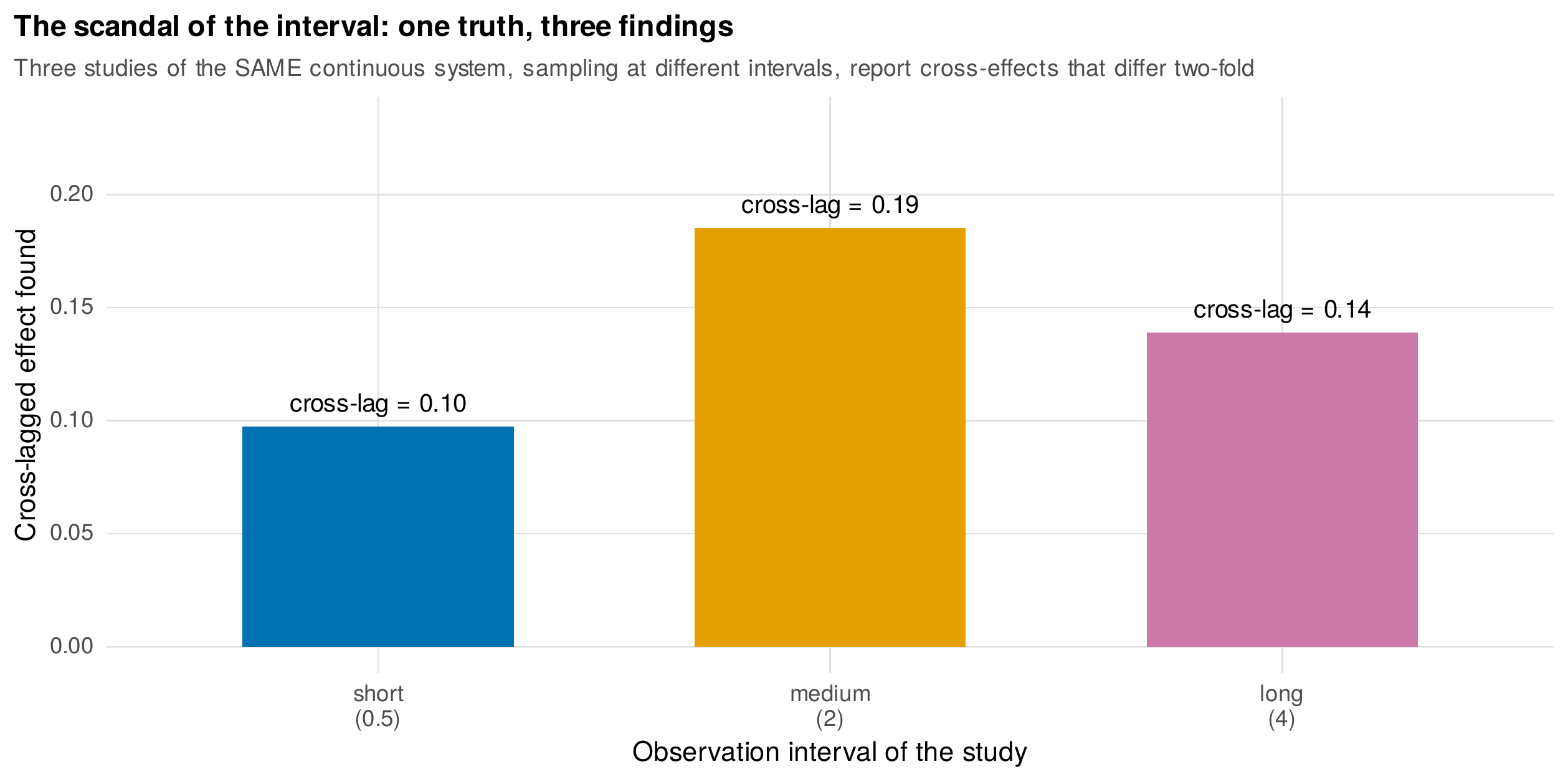
Note. Three studies of the same continuous-time system, sampling at intervals of \(0.5\), \(2\), and \(4\) time units, report cross-lagged effects that differ roughly two-fold. None is wrong; each reads the same underlying process at a different interval. The discrete cross-lag is meaningless without its interval.
The relation that generates this behavior is the chapter’s master equation, and it is worth meeting numerically before formally. If the underlying continuous dynamics are governed by a drift matrix \(\mathbf{A}\), then the discrete transition matrix over an interval \(\Delta t\), the matrix of autoregressions and cross-lags a discrete model would estimate at that spacing, is the matrix exponential \(\boldsymbol{\Phi}(\Delta t) = e^{\mathbf{A}\Delta t}\). Feeding a single drift matrix through this relation at a range of intervals produces the effect-versus-interval curves of Figure 27.2, the central graphic of the chapter and the one to internalize. The auto-effects, the diagonal entries, decay monotonically from one toward zero as the interval grows, because a variable’s dependence on its own distant past fades. The cross-effect, the off-diagonal, does something more interesting: it starts near zero at very short intervals, because an influence has had no time to accumulate, rises to a peak at an intermediate interval, here near \(\Delta t = 2\), and then declines as the whole system washes out. A study sampling at a very short interval finds almost no cross-effect and might conclude there is none; a study at the peak finds it strong; a study at a long interval finds it weakening again. There is an optimal interval at which an effect is most detectable, a point developed by Dormann and Griffin (2015), and the single number a discrete study reports is just one sample from this curve. In systems with feedback the two cross-effects can even change their ordering across intervals, so that which variable appears to lead depends on the spacing, a hazard analyzed by Kuiper and Ryan (2018). This reframes the interval caveats raised for the latent change score in Chapter 20, the cross-study comparability problem of Chapter 21, and the discretization coarseness of Chapter 25, all as facets of one underlying truth.
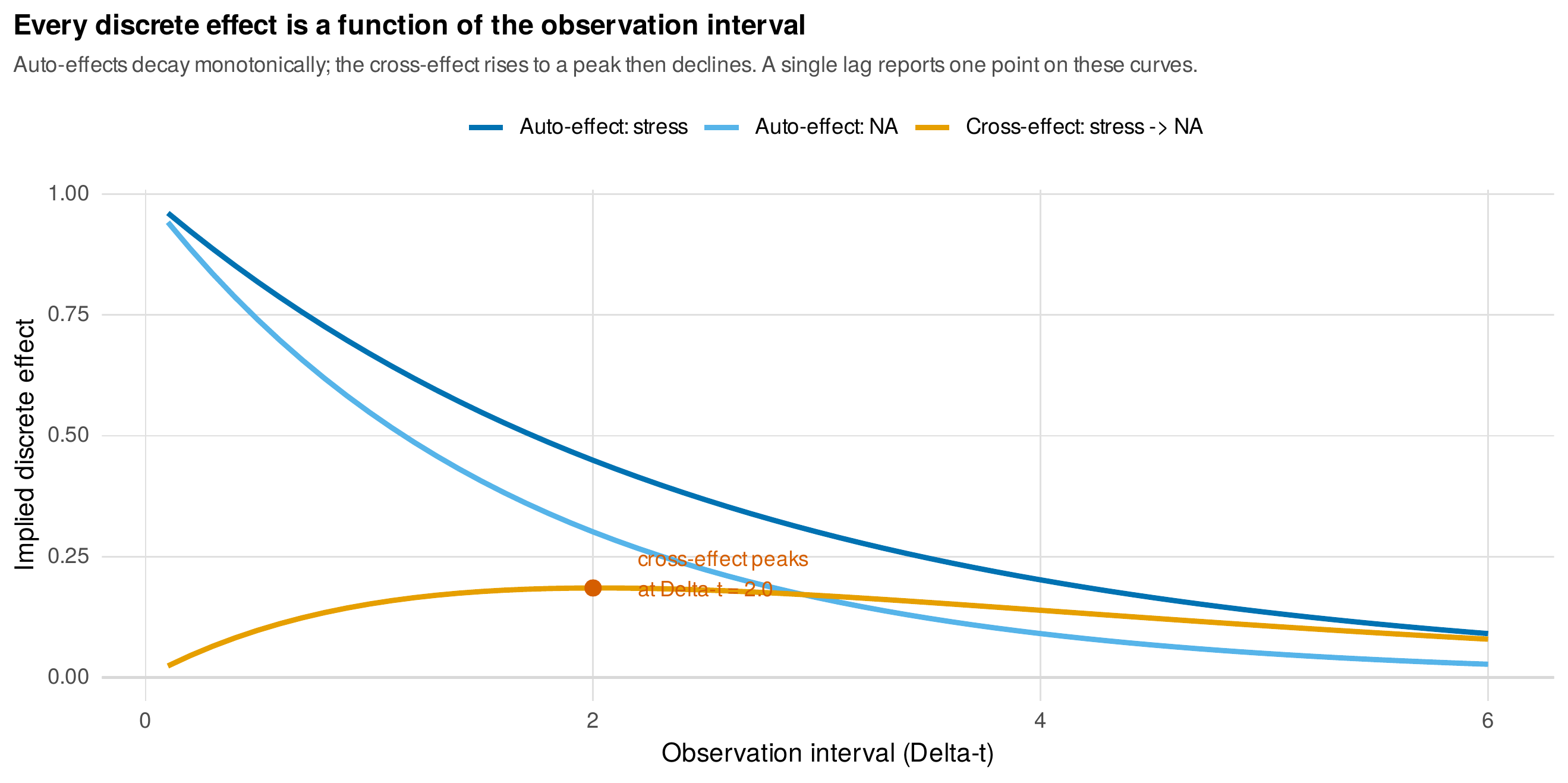
Note. Discrete auto-effects and cross-effects implied by a fixed drift matrix, as functions of the interval \(\Delta t\), via \(\boldsymbol{\Phi}(\Delta t) = e^{\mathbf{A}\Delta t}\). Auto-effects decay monotonically; the cross-effect rises to a peak near \(\Delta t = 2\) and then declines. Any discrete study reports a single point on these curves. This is the chapter’s reflex figure.
27.2 The Continuous-Time Model
The model underneath the curves is a stochastic differential equation, and its symbols carry psychological meaning that survives the formalism. Writing \(\boldsymbol{\eta}(t)\) for the vector of latent states at continuous time \(t\), the equation \(d\boldsymbol{\eta}(t) = \big(\mathbf{A}\,\boldsymbol{\eta}(t) + \mathbf{b}\big)\,dt + \mathbf{G}\,d\mathbf{W}(t)\) has three parts. The drift term \(\mathbf{A}\,\boldsymbol{\eta}(t)\,dt\) is the deterministic pull: at any instant the system is drawn in a direction set by the drift matrix acting on the current state, and for a mean-reverting process this pull is back toward equilibrium. The intercept \(\mathbf{b}\) locates that equilibrium. The diffusion term \(\mathbf{G}\,d\mathbf{W}(t)\) is the ongoing stochastic input, the continuous analogue of the innovations, where \(\mathbf{W}(t)\) is a Wiener process, a random walk in continuous time whose increments are independent and Gaussian, the source of the perpetual small shocks that keep the system alive. No measure theory is needed to use the model; the drift is where the system is pulled, and the diffusion is how hard it is jostled along the way.
The drift matrix is the object to interpret, and its diagonal is the most interpretable currency the chapter offers. A negative diagonal entry \(a_{ii}\) is a mean-reversion rate: the more negative it is, the faster the variable is pulled back to equilibrium after a perturbation. That rate translates into a half-life, the time for a disturbance to decay to half its size, given by \(\ln 2 / |a_{ii}|\), the same interpretive move Chapter 24 made for the autoregression but now in continuous time and independent of any sampling interval. A drift auto-effect of \(-0.40\) is a half-life of \(1.73\) time units; one of \(-0.60\) is a half-life of \(1.16\). The off-diagonal entries are continuous-time cross-effects, the instantaneous coupling of one variable to another, and they carry the same interpretive discipline as the discrete cross-lags of Chapter 25: they are conditional, system-embedded quantities, not isolated causal arrows, and they must not be compared across variables measured on different scales without standardization. Table 27.1 sets the continuous and discrete vocabularies side by side, and Table 27.2 interprets the drift parameters with their half-lives.
Table 27.1. Discrete and continuous-time correspondence.
| Discrete-time object | Continuous-time object | Relation |
|---|---|---|
| Transition matrix \(\boldsymbol{\Phi}(\Delta t)\) | Drift matrix \(\mathbf{A}\) | \(\boldsymbol{\Phi}(\Delta t) = e^{\mathbf{A}\Delta t}\) |
| Autoregression \(\phi_{ii}(\Delta t)\) | Mean-reversion rate \(a_{ii}<0\) | Half-life \(\ln 2 / |a_{ii}|\) |
| Cross-lag \(\phi_{ij}(\Delta t)\) | Continuous cross-effect \(a_{ij}\) | Nonmonotonic in \(\Delta t\) |
| Innovation covariance \(\mathbf{Q}(\Delta t)\) | Diffusion \(\mathbf{G}\mathbf{G}^{\top}\) | Van Loan integral |
| Intercept | Equilibrium \(-\mathbf{A}^{-1}\mathbf{b}\) | Long-run mean |
Note. The drift matrix is the interval-free parameterization; the discrete transition at any spacing is recovered by the matrix exponential. The diffusion is the continuous-time source of the innovation covariance, which itself depends on the interval.
Table 27.2. Interpreting the drift matrix, with half-lives.
| Drift entry | Value | Half-life | Reading |
|---|---|---|---|
| \(a_{\text{stress}}\) (auto) | \(-0.40\) | \(1.73\) | Stress reverts to equilibrium with a half-life of \(1.73\) units |
| \(a_{\text{na}}\) (auto) | \(-0.60\) | \(1.16\) | Negative affect reverts faster, half-life \(1.16\) |
| \(a_{\text{na,stress}}\) (cross) | \(+0.25\) | — | Stress continuously pushes negative affect upward |
| \(a_{\text{stress,na}}\) (cross) | \(0.00\) | — | No feedback from affect to stress in this system |
Note. Auto-effects are mean-reversion rates read as half-lives, the interval-free interpretable currency. Cross-effects are continuous couplings whose discrete magnitude at any interval follows the effect-versus-interval curve. Values from ct_sim.
The reason continuous time subsumes any spacing is the exact discrete solution. Over an interval \(\Delta t\), the process satisfies \(\boldsymbol{\eta}_{t} = e^{\mathbf{A}\Delta t}\,\boldsymbol{\eta}_{t-1} + \mathbf{w}_t\) exactly, with \(\mathbf{w}_t\) Gaussian with a covariance that is itself an integral of the diffusion over the interval, computed by the Van Loan method the foundations box records. This means the same drift matrix generates the correct discrete dynamics at every interval simultaneously, so a dataset with mixed spacings, short gaps within a day and a long gap overnight, is handled without pretending the gaps are equal. The measurement layer is exactly the state-space observation equation of Chapter 26: the continuous state is observed through a loading matrix with measurement error, and the engine that fits the model is the Kalman filter of that chapter with a transition matrix recomputed from the drift at each occasion’s interval. The Ornstein-Uhlenbeck process, the continuous-time AR(1), is the scalar case and the one to build intuition on. Figure 27.3 shows its sample paths: each is pulled back toward the equilibrium at a rate set by the auto-effect, perpetually knocked away by the diffusion and perpetually drawn back, with the half-life marking how quickly a departure decays. The stationary distribution has a variance the foundations box gives, and the whole picture formalizes the vector-field and attractor intuitions previewed in Chapters 9 and 20.
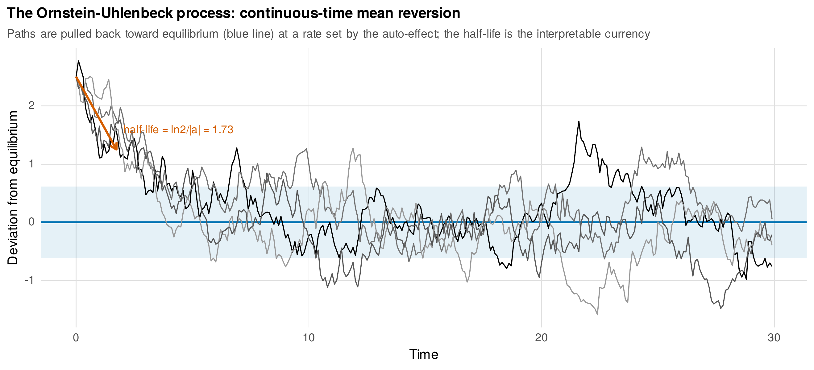
Note. Four sample paths of an Ornstein-Uhlenbeck process, the continuous-time AR(1). Each is pulled toward equilibrium (blue line) at the rate set by the auto-effect and jostled by the diffusion; the shaded band is one stationary standard deviation. The half-life, the red arrow, is the interpretable summary of the reversion rate.
Foundations Box • The matrix exponential, the exact discrete solution, and the OU variance
The matrix exponential is defined by the same series as the scalar one, \(e^{\mathbf{A}\Delta t} = \mathbf{I} + \mathbf{A}\Delta t + \tfrac{1}{2}(\mathbf{A}\Delta t)^2 + \tfrac{1}{6}(\mathbf{A}\Delta t)^3 + \cdots\), and for a diagonalizable drift \(\mathbf{A} = \mathbf{V}\boldsymbol{\Lambda}\mathbf{V}^{-1}\) it is computed cleanly as \(\mathbf{V}\,e^{\boldsymbol{\Lambda}\Delta t}\,\mathbf{V}^{-1}\), where \(e^{\boldsymbol{\Lambda}\Delta t}\) just exponentiates the eigenvalues. For the scalar drift \(a = -0.40\) and \(\Delta t = 2\) this gives \(e^{-0.8} = 0.449\), the discrete autoregression a two-unit-lag study would estimate. The exact discrete solution follows: integrating the stochastic differential equation over \([t-\Delta t, t]\) gives \(\boldsymbol{\eta}_t = e^{\mathbf{A}\Delta t}\boldsymbol{\eta}_{t-1} + \mathbf{w}_t\) with \(\mathrm{Cov}(\mathbf{w}_t) = \int_0^{\Delta t} e^{\mathbf{A}s}\,\mathbf{G}\mathbf{G}^{\top}\,e^{\mathbf{A}^{\top}s}\,ds\), the integrated diffusion, obtained without numerical integration by the Van Loan trick: exponentiate the block matrix \(\left[\begin{smallmatrix} -\mathbf{A} & \mathbf{G}\mathbf{G}^{\top} \\ \mathbf{0} & \mathbf{A}^{\top}\end{smallmatrix}\right]\Delta t\) and read the covariance from its upper-right block times the transition. For the scalar Ornstein-Uhlenbeck process the stationary variance is \(\sigma^2 = -g^2/(2a)\), so a stronger reversion (more negative \(a\)) or a weaker diffusion gives a tighter equilibrium band, the continuous-time analogue of \(\sigma^2_\varepsilon/(1-\phi^2)\).
The character of the whole system is decided by the eigenvalues of the drift matrix, which is where continuous time makes contact with the oscillators of Chapter 32. Figure 27.4 shows two systems. When the eigenvalues are real and negative, the system decays smoothly back to equilibrium after a perturbation, the mean-reverting behavior of the worked example. When the eigenvalues are complex, with negative real parts and nonzero imaginary parts, the system oscillates as it returns, overshooting the equilibrium and swinging back in a damped rhythm, the continuous-time face of the second-order oscillation Chapter 24 met and the bridge to the differential-equation oscillators of Chapter 32. The real part of the eigenvalue governs how fast the system settles, the imaginary part how fast it oscillates. Figure 27.5 draws the same dynamics as a vector field, each arrow the instantaneous pull the drift matrix exerts at that point in the state space, all of them flowing toward the equilibrium and bent by the cross-effect, which formalizes the attractor pictures the book has shown in preview since Chapter 9.
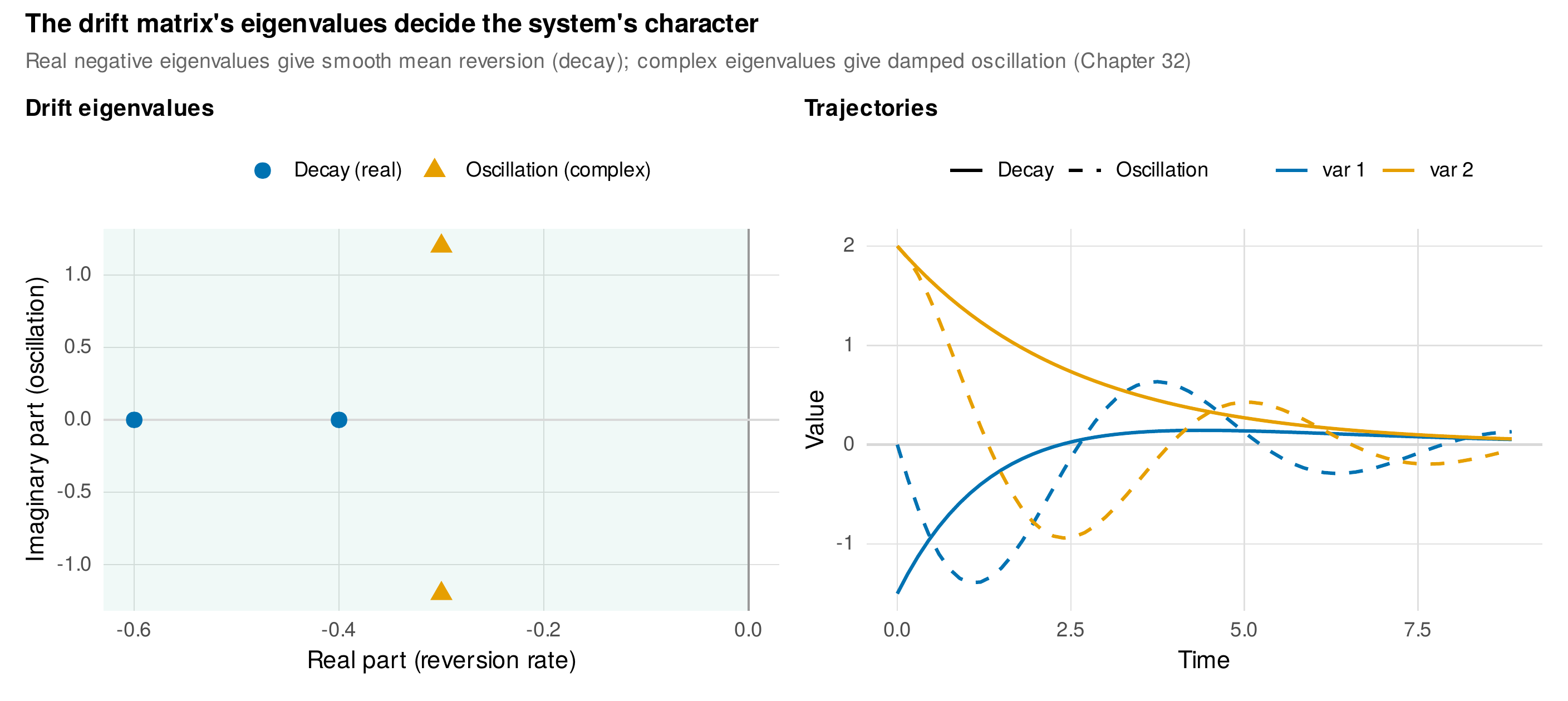
Note. Left: eigenvalues of a decay system (real, negative) and an oscillatory system (complex) in the plane; the shaded region marks stability (negative real parts). Right: the trajectories each produces, a smooth return versus a damped oscillation. The imaginary part of the eigenvalue is the source of oscillation, the bridge to Chapter 32.
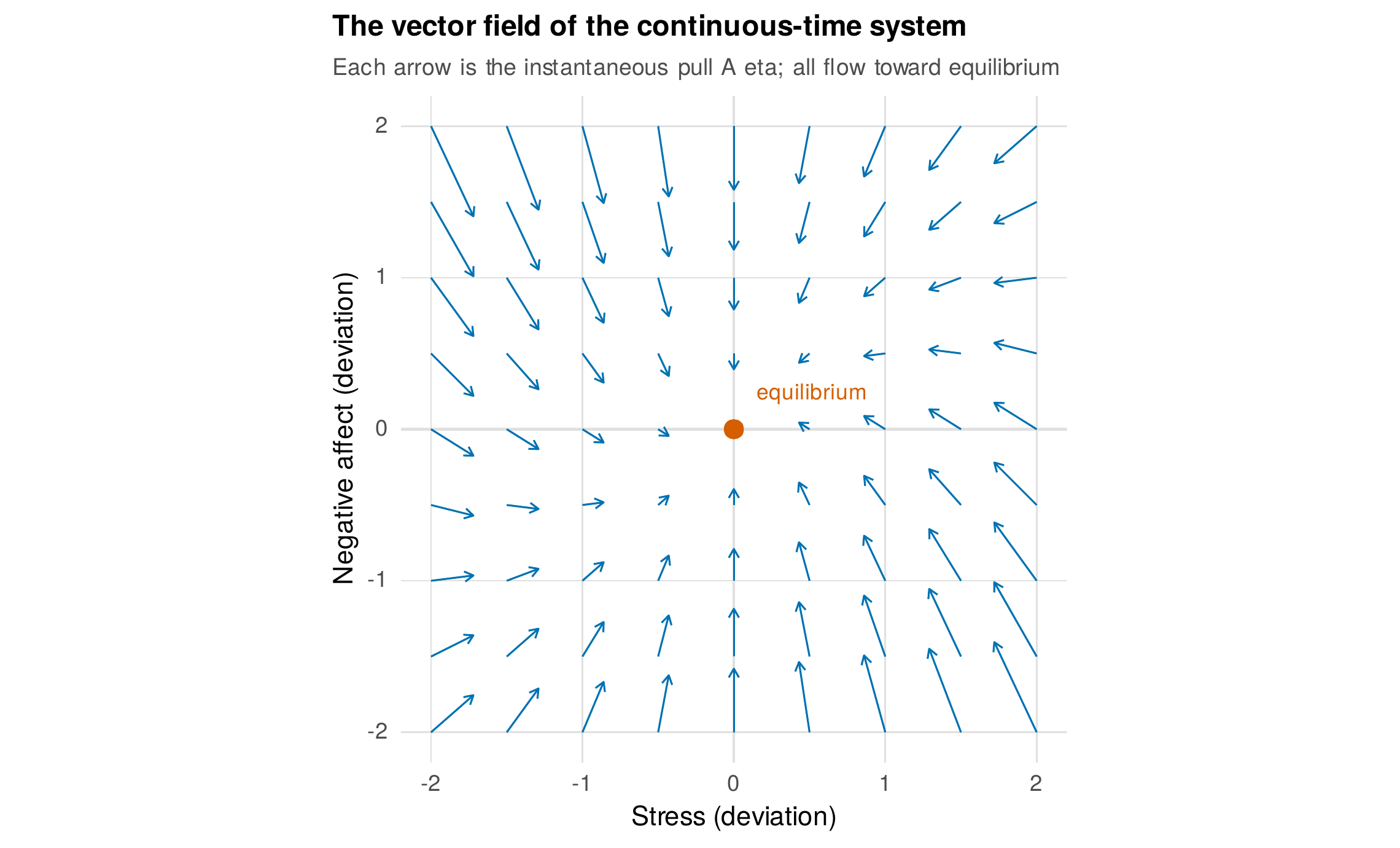
Note. Each arrow is the instantaneous pull \(\mathbf{A}\boldsymbol{\eta}\) the drift exerts at that state; all flow toward the equilibrium (red point). The asymmetry, the bending of the flow, is the stress-to-affect cross-effect. This is the formal version of the attractor previews of Chapters 9 and 20.
27.3 Fitting Continuous-Time Models
The production tool for these models is the ctsem package, which specifies a continuous-time model, fits it either by frequentist Kalman maximum likelihood or in a Stan-based hierarchical Bayesian mode, and returns the drift matrix with its uncertainty. The analyses here are built from a hand-rolled continuous-time engine, the matrix exponential for the transition, the Van Loan integral for the process covariance, and a time-varying version of Chapter 26’s Kalman filter that recomputes both at each occasion’s interval, so that the mechanics are auditable against a known truth; ctsem is the tool to reach for in applied work, and Table 27.3 records its modes. The first rung of the worked ladder is recovery. Simulating a bivariate continuous-time process with a known drift matrix, sampled at irregular intervals, and fitting the continuous-time model by maximum likelihood recovers the drift: the auto-effects come back as \(-0.45\) and \(-0.56\) against the generating \(-0.40\) and \(-0.60\), the stress-to-affect cross-effect as \(0.29\) against \(0.25\), and the half-lives as \(1.55\) and \(1.25\) units against the true \(1.73\) and \(1.16\), close given the single series. The estimator recovers the interval-free dynamics from unequally spaced data, which is the whole point.
# The lag-translator and a continuous-time fit (hand-rolled engine)
library(Matrix)
A <- matrix(c(-0.40, 0.00,          # drift: negative diagonals = reversion rates
               0.25, -0.60), 2, 2, byrow = TRUE)
Phi <- function(dt) as.matrix(expm(A * dt))       # discrete effects at interval dt
Phi(0.5); Phi(2); Phi(4)            # the effect-vs-interval curve, one dt at a time
log(2) / abs(diag(A))               # half-lives: 1.73 and 1.16 time units
# fit a CT-VAR to irregularly spaced data by transition ML (ct_fit_bivar in the
# analysis script): precompute Phi(dt) and the Van Loan Q*(dt) per unique interval,
# then maximize the Gaussian transition likelihood over A and the diffusion.
fit <- ct_fit_bivar(Y = as.matrix(ct_sim[, c("stress","na")]), dtv = ct_sim$dt)
fit$A; fit$half_life                # recovered drift and half-lives
The second rung is the person: fitting a continuous-time AR(1) to each individual’s series recovers a person-specific reversion rate and therefore a person-specific half-life, and the distribution of those half-lives is an individual-differences finding in the currency of dynamics. Figure 27.6 shows both the real-data distribution and its validation. On the affect_ema data, using each person’s actual beep timestamps with their two-and-a-half-hour within-day gaps and eleven-and-a-half-hour overnight gaps, the negative-affect half-lives spread widely, with a median near three hours and a ten-to-ninety-percent range from under an hour to nearly eight, so people differ substantially in how quickly their affect returns to baseline. That the estimator can recover such heterogeneity is confirmed by simulation: generating people with known, varying reversion rates and re-estimating each recovers the true half-lives with a correlation of \(0.63\), imperfect at the short series lengths of a diary study but clearly informative. In the hierarchical Bayesian mode of ctsem these person-specific parameters are estimated jointly with a population distribution over them, the same borrowing of strength as the random effects of Chapter 25, and the same two people whose random autoregressions opened that chapter reappear here as draws from a distribution of drift matrices.
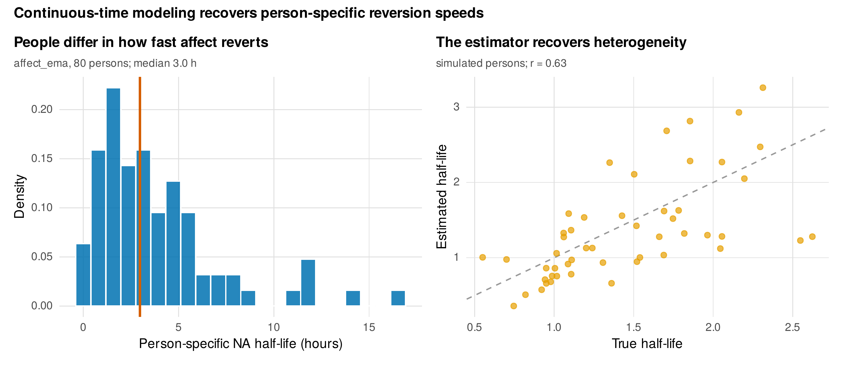
Note. Left: the distribution of person-specific negative-affect half-lives from continuous-time AR(1) fits to affect_ema, using each person’s real irregular timestamps; the median is near three hours. Right: a simulation validation, estimated against true half-lives across people, recovering the heterogeneity with a correlation of \(0.63\).
The third rung is the deliberate demonstration that continuous time is not only for intensive data: it repairs panel studies too. A panel with only a handful of waves, but with those waves falling at genuinely different real times across people, some measured a month apart and others three months apart, is exactly the situation a discrete model mishandles, because it applies one lag coefficient to intervals that are not equal. Figure 27.7 shows the timing raster, each person’s waves at their own times, alongside the consequence. A discrete model that pretends the spacing is equal reports a single cross-lag of \(0.14\), one number, whereas the true cross-effect actually varies across the intervals present in the data, from about \(0.10\) at the shortest spacings to \(0.18\) at the longest, a range the pretense collapses into a value that matches no interval anyone observed. The continuous-time model recovers the drift matrix that generates all of these correctly, and its reading against the random-intercept cross-lagged panel model of Chapter 21 is that continuous time adds exactly what unequal spacing across persons demands. The applied output of any continuous-time fit is therefore never the raw drift alone but its translation: the implied discrete matrices at the intervals a reader cares about, the half-lives with their intervals of uncertainty, and the effect-versus-interval curve, so that the result is comparable to studies at other spacings.
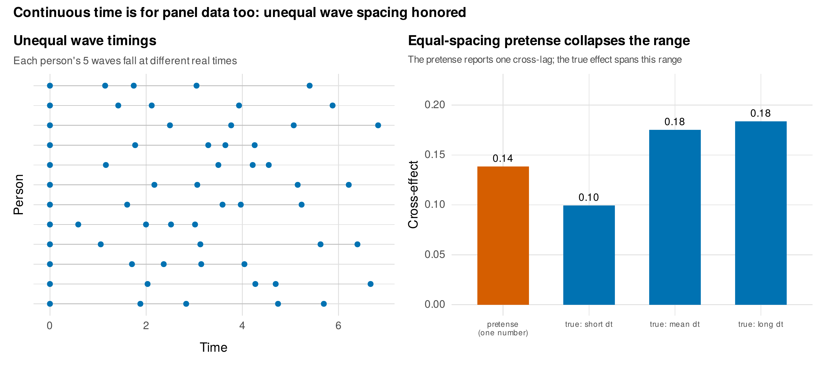
Note. Left: a raster of person-specific wave timings in a five-wave panel; each person’s waves fall at different real times. Right: a discrete model pretending equal spacing reports one cross-lag (\(0.14\)), while the true cross-effect spans \(0.10\) to \(0.18\) across the intervals actually present. Continuous time honors the unequal spacing.
27.4 Limits, Honesty, and Choices
Continuous time is powerful but not omnipotent, and its most important limit is the one Chapter 1 previewed under the name aliasing, now given the matrix-exponential lens. A process that operates much faster than it is sampled cannot be recovered, because between two observations the fast dynamics have run their course and the observations look nearly independent, carrying no information about the reversion rate. Figure 27.8 makes this quantitative: estimating the reversion rate of a fast process at a range of sampling intervals, the half-life is recovered well while the sampling interval is shorter than the process half-life, but as the interval grows past the half-life the estimate degrades and its uncertainty explodes, until at an interval several times the half-life the drift is effectively unidentifiable. The practical reading is that the sampling rate must be matched to the timescale of the process one hopes to study, a design decision no analysis can repair after the fact. Two further limits bound the scope. The model as presented is linear, and processes with genuinely nonlinear dynamics, thresholds, or state-dependent reversion require the nonlinear extensions of Chapter 32. And the process is assumed stationary around a fixed equilibrium; continuous-time growth models that let the equilibrium itself move exist and are cited, but the workhorse assumes a stable attractor.
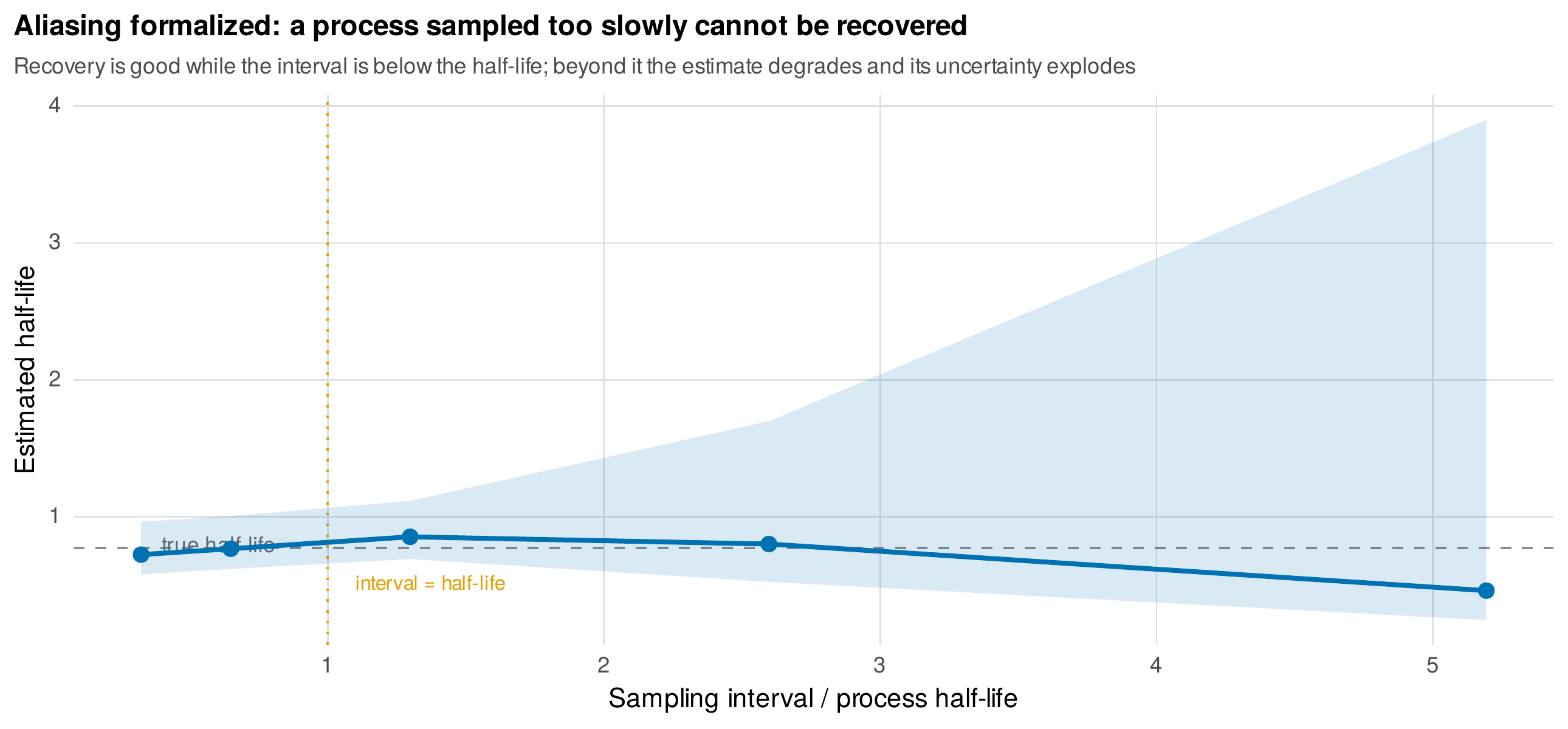
Note. The estimated half-life of a fast process against the ratio of the sampling interval to the true half-life. Recovery is good while the interval is below the half-life (ratio under one); beyond it the estimate degrades and its uncertainty, the shaded band, explodes. Sampling rate must match the process timescale.
The decision of when to pay the conceptual cost of continuous time follows from the interval structure of the data, and Figure 27.9 lays it out. When the intervals within or across people vary substantially, continuous time is worth it, because the alternatives misrepresent the dynamics. When the intervals are equal or nearly so, a discrete model is adequate and simpler, and the TINTERVAL discretization of Chapter 25’s dynamic structural equation modeling is a middle path that aligns modestly unequal intervals to a fine grid without the full continuous-time apparatus. The equal-spacing pretense is tolerable only when the interval variance is small, and the chapter’s simulations quantify when it is not: with the wide spacing variation of the panel example, the pretense missed the interval-specific effects substantially. The larger vision, and the reason the overhead is worth learning, is comparability. A drift matrix is interval-free, so it is the natural common currency for comparing studies that used different designs and for the meta-analysis of dynamics, an active program that seeks to pool drift matrices across studies the way ordinary meta-analysis pools effect sizes. Table 27.4 gives the decision in tabular form and Table 27.5 the reporting checklist, whose non-negotiable element is the implied-interval translation.
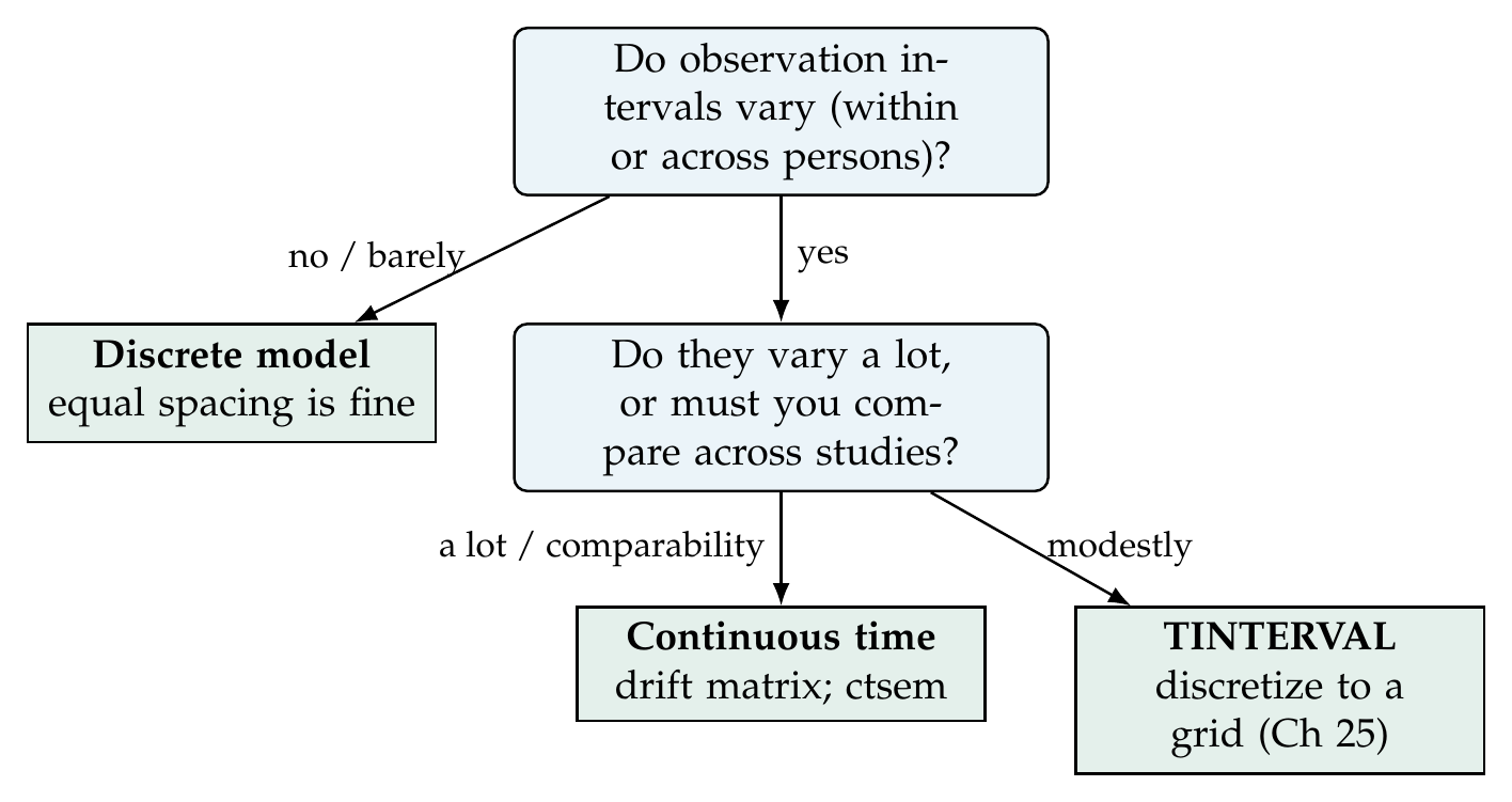
Note. Equal or nearly equal intervals permit a discrete model; modestly unequal intervals can be handled by the TINTERVAL discretization of Chapter 25; substantially unequal intervals, or the need to compare across studies, call for the continuous-time drift matrix. The cost is conceptual overhead; the payoff is comparability.
Table 27.3. ctsem modes and settings.
| Mode / setting | What it does | Guidance |
|---|---|---|
| Frequentist (Kalman ML) | Maximum-likelihood drift, fast | Good for N=1 and single-group panel; delta-method intervals |
| Hierarchical Bayesian | Random drift across persons via Stan | Person-specific dynamics with pooling; needs priors and runtime |
| Priors (hierarchical) | Weakly informative on drift/diffusion | Report them; probe sensitivity (Ch 17 literacy) |
| Time data | Actual observation times supplied | The interval structure is data, not an assumption |
| Output translation | Implied discrete matrices at chosen \(\Delta t\) | Always report; the drift alone is not reader-ready |
Note. The frequentist mode fits a fixed drift quickly; the hierarchical Bayesian mode estimates person-specific drift with a population distribution, inheriting the Bayesian workflow of Chapter 17. Verify the current package interface at analysis time.
Table 27.4. When continuous time matters.
| Situation | Interval structure | Recommendation |
|---|---|---|
| Equal-spaced panel or ILD | Constant \(\Delta t\) | Discrete model suffices; report the interval |
| Mildly unequal spacing | Small interval variance | Discrete or TINTERVAL (Ch 25); check sensitivity |
| Strongly unequal spacing | Large interval variance | Continuous time; the pretense misleads |
| Comparing across studies | Different intervals by design | Continuous time; drift is the common currency |
| Fast process, coarse sampling | Interval \(\gg\) half-life | No model recovers it; fix the design |
Note. The equal-spacing pretense is tolerable only when the interval variance is small. Substantial variation, or cross-study comparison, is where the drift matrix earns its overhead. No estimator overcomes sampling that is too slow for the process.
Common Pitfall • Three ways continuous-time results are misread
First, interpreting the drift cross-effects as though they were discrete cross-lags: the continuous cross-effect at an instant is not the number a discrete study reports at its interval, and the two are related only through the effect-versus-interval curve, so a drift entry of \(0.25\) is not a “cross-lag of \(0.25\)” at any particular spacing. Second, comparing raw drift entries across variables measured on different scales, which is as meaningless in continuous time as comparing unstandardized regression coefficients across predictors on different metrics; standardize the drift before comparing auto- or cross-effects across variables. Third, believing that continuous time fixes confounding: it fixes the interval problem, recovering interval-free dynamics, but it does nothing about an omitted variable that drives two of the modeled ones, so the caution ledger of Chapters 25 and 26 transfers intact, and a continuous-time cross-effect is a predictive, system-embedded quantity, not a license for a causal claim.
In Practice • Starting values, priors, and the oscillation-versus-noise problem
Give the optimizer sensible starting values for the drift by first fitting a discrete model at the mean interval and taking the matrix logarithm of its transition, divided by that interval, as an initial drift; a cold start from arbitrary values often fails to converge. In the hierarchical Bayesian mode, place weakly informative priors on the drift diagonals that respect their sign, mean reversion means negative, and on the diffusion, and report and probe them. The hardest identification problem at psychological series lengths is distinguishing genuine oscillation, complex drift eigenvalues, from noise: a short, noisy series can show apparent cycles that are sampling artifacts, so an oscillatory drift should be accepted only when it survives a sensitivity check and, ideally, replicates across persons, and the estimate of an oscillation frequency near the sampling rate should be treated with the aliasing warning firmly in mind.
Software Note • Continuous-time software
The primary tool is ctsem, which specifies continuous-time structural equation models and fits them in two modes, a fast frequentist Kalman-maximum-likelihood mode and a Stan-based hierarchical Bayesian mode that estimates person-specific drift matrices with a population distribution; the package takes the actual observation times as input, so unequal spacing is handled natively. The dynr package of Chapter 26 also has continuous-time capabilities and adds regime-switching, and OpenMx can express continuous-time models through its state-space machinery. Mplus, by contrast, does not currently fit genuine continuous-time models, offering the TINTERVAL discretization of its dynamic structural equation modeling as the nearest approximation, which aligns unequal intervals to a fine grid rather than parameterizing the underlying differential equation. The analyses in this chapter used none of these, building the continuous-time engine from the matrix exponential, the Van Loan integrated diffusion, and a time-varying Kalman filter, so that every relation could be checked against a known drift matrix; the packages are the right choice for applied work, and their interfaces should be verified at analysis time, as this is an actively developing area.
Writing up a continuous-time analysis has one non-negotiable requirement that distinguishes it from every discrete report: the results must be given in a form that is interval-free and then translated to intervals a reader can use. The report should present the drift matrix with its uncertainty, the auto-effects rendered as half-lives with their intervals, and the cross-effects with the caution that they are continuous couplings, not discrete cross-lags. It should then translate: the implied discrete transition matrices at one or two substantively meaningful intervals, and ideally the effect-versus-interval curve itself, so that the finding can be compared to studies at other spacings. It should state the observation-time structure that was modeled, note whether the frequentist or hierarchical mode was used with its priors, and confront the sampling-rate limit honestly, acknowledging which timescales the design could and could not resolve. A model sentence reads: “A bivariate continuous-time model was fit to the irregularly spaced data with the drift matrix estimated by maximum likelihood. Negative affect reverted to equilibrium with a half-life of \(1.25\) time units (roughly three hours in the diary data) and stress with a half-life of \(1.55\); stress exerted a positive continuous-time effect on negative affect whose implied discrete cross-lag peaks near a two-unit interval. Because the effect depends on the interval, we report the implied discrete matrices at one- and four-unit spacings so the estimates can be compared with studies using those lags.”
Table 27.5. Continuous-time reporting checklist.
| Element | What to report |
|---|---|
| Drift matrix | Estimates with uncertainty; the interval-free parameterization |
| Half-lives | Auto-effects as \(\ln 2 / |a_{ii}|\) with intervals, in interpretable time units |
| Cross-effects | Continuous couplings, flagged as not discrete cross-lags |
| Implied discrete matrices | \(\boldsymbol{\Phi}(\Delta t)\) at one or two substantive intervals (mandatory) |
| Effect-vs-interval curve | The cross-effect across intervals, ideally shown |
| Observation times | The interval structure modeled; irregular spacing acknowledged |
| Estimation | Frequentist or hierarchical mode; priors if Bayesian |
| Sampling-rate honesty | Which process timescales the design could resolve |
Note. The mandatory element is the implied-interval translation: a drift matrix reported without its discrete implications at named intervals is not reader-ready, because comparability, the reason for continuous time, requires it.
Chapter Summary
Discrete-time dynamic coefficients depend on the observation interval, so studies at different spacings estimate different numbers and can disagree about which variable leads, a threat to the comparability of a literature rather than a footnote. The continuous-time model removes the dependence by parameterizing the underlying process with a drift matrix and treating observation times as data, and the discrete effect at any interval is recovered from the drift by the matrix exponential \(\boldsymbol{\Phi}(\Delta t) = e^{\mathbf{A}\Delta t}\), whose effect-versus-interval curves show auto-effects decaying monotonically and cross-effects rising to a peak before declining, so a single lag reports one point on a curve. The drift matrix’s negative diagonals are mean-reversion rates read as half-lives, the interval-free interpretable currency, and its off-diagonals are continuous couplings; its eigenvalues decide whether the system decays or oscillates, the bridge to Chapter 32. The exact discrete solution, the transition by matrix exponential and the process covariance by the Van Loan integral, lets one drift matrix generate the correct dynamics at every spacing, so mixed and unequal intervals are handled without pretending they are equal, and the fitting engine is Chapter 26’s Kalman filter with a transition recomputed per interval. The estimator recovers a known drift from irregular data on ct_sim, recovers person-specific half-lives whose spread on affect_ema is a real individual-differences finding, and repairs panel studies with unequal wave spacing that a discrete model, collapsing a range of true effects into one wrong number, mishandles. The limits are honest: a process sampled much slower than its half-life is aliased and unrecoverable, the linear stationary model has a scope, and continuous time fixes intervals, not omitted-variable confounding. The decision to use it follows the interval structure, and its payoff is the drift matrix as a common currency for comparing and pooling dynamics across studies, which is why every continuous-time report must translate its drift into implied discrete effects at named intervals.
Bergstrom, A. R. (1988). The history of continuous-time econometric models. Econometric Theory, 4(3), 365–383. https://doi.org/10.1017/S0266466600013359
Boker, S. M. (2001). Differential structural equation modeling of intraindividual variability. In L. M. Collins & A. G. Sayer (Eds.), New methods for the analysis of change (pp. 5–27). American Psychological Association. https://doi.org/10.1037/10409-001
Deboeck, P. R., & Preacher, K. J. (2016). No need to be discrete: A method for continuous time mediation analysis. Structural Equation Modeling: A Multidisciplinary Journal, 23(1), 61–75. https://doi.org/10.1080/10705511.2014.973960
Dormann, C., & Griffin, M. A. (2015). Optimal time lags in panel studies. Psychological Methods, 20(4), 489–505. https://doi.org/10.1037/met0000041
Driver, C. C., Oud, J. H. L., & Voelkle, M. C. (2017). Continuous time structural equation modeling with R package ctsem. Journal of Statistical Software, 77(5), 1–35. https://doi.org/10.18637/jss.v077.i05
Driver, C. C., & Voelkle, M. C. (2018). Hierarchical Bayesian continuous time dynamic modeling. Psychological Methods, 23(4), 774–799. https://doi.org/10.1037/met0000168
Hecht, M., & Zitzmann, S. (2021). Sample size recommendations for continuous-time models: Compensating shorter time series with larger numbers of persons and vice versa. Structural Equation Modeling: A Multidisciplinary Journal, 28(2), 229–236. https://doi.org/10.1080/10705511.2020.1779069
Kuiper, R. M., & Ryan, O. (2018). Drawing conclusions from cross-lagged relationships: Re-considering the role of the time-interval. Structural Equation Modeling: A Multidisciplinary Journal, 25(5), 809–823. https://doi.org/10.1080/10705511.2018.1431046
Oravecz, Z., Tuerlinckx, F., & Vandekerckhove, J. (2009). A hierarchical Ornstein–Uhlenbeck model for continuous repeated measurement data. Psychometrika, 74(3), 395–418. https://doi.org/10.1007/s11336-008-9106-8
Oravecz, Z., Tuerlinckx, F., & Vandekerckhove, J. (2011). A hierarchical latent stochastic differential equation model for affective dynamics. Psychological Methods, 16(4), 468–490. https://doi.org/10.1037/a0024375
Oud, J. H. L., & Jansen, R. A. R. G. (2000). Continuous time state space modeling of panel data by means of SEM. Psychometrika, 65(2), 199–215. https://doi.org/10.1007/BF02294374
Ryan, O., Kuiper, R. M., & Hamaker, E. L. (2018). A continuous-time approach to intensive longitudinal data: What, why, and how? In K. van Montfort, J. H. L. Oud, & M. C. Voelkle (Eds.), Continuous time modeling in the behavioral and related sciences (pp. 27–54). Springer. https://doi.org/10.1007/978-3-319-77219-6_2
Uhlenbeck, G. E., & Ornstein, L. S. (1930). On the theory of the Brownian motion. Physical Review, 36(5), 823–841. https://doi.org/10.1103/PhysRev.36.823
van Montfort, K., Oud, J. H. L., & Voelkle, M. C. (Eds.). (2018). Continuous time modeling in the behavioral and related sciences. Springer. https://doi.org/10.1007/978-3-319-77219-6
Voelkle, M. C., & Oud, J. H. L. (2013). Continuous time modelling with individually varying time intervals for oscillating and non-oscillating processes. British Journal of Mathematical and Statistical Psychology, 66(1), 103–126. https://doi.org/10.1111/j.2044-8317.2012.02043.x
Voelkle, M. C., Oud, J. H. L., Davidov, E., & Schmidt, P. (2012). An SEM approach to continuous time modeling of panel data: Relating authoritarianism and anomia. Psychological Methods, 17(2), 176–192. https://doi.org/10.1037/a0027543