Chapter 28
Network Approaches to Intensive Longitudinal Data
The models of the preceding chapters treated the covariation among psychological variables as something to be explained, usually by a latent common cause that the variables measure. The network approach inverts the picture. It treats the variables, symptoms, moods, behaviors, as a system of components that directly influence one another, so that a syndrome is not the reflection of an underlying entity but an emergent pattern of interactions, a feedback structure that can settle into stable states and be pushed between them. This reframing has energized clinical and personality psychology, because it promises intervention targets, an account of comorbidity as bridges between clusters, and person-specific etiologies, and because its central object, the estimated network, is a vivid and shareable picture. The pictures are also the danger. An edge in an estimated network is a conditional association, not a causal path; a central node is a topological summary, not a proven lever; and a network estimated from a modest sample can fail to replicate in ways a compelling layout conceals. This chapter teaches the machinery at full strength and the discipline at full strength together. It builds the Gaussian graphical model and its regularized estimation, maps the intensive-longitudinal network triptych exactly onto Chapter 25’s matrices so that one set of objects wears two vocabularies, and then, in the exhibit that is the book’s distinctive contribution here, audits an estimated network against a known truth to show that recovery is partial rather than perfect. It treats the replicability and centrality controversies as content, gives person-specific structure its own method, and closes with a claims ladder that fixes the language a network result has earned to the evidence that supports it.
Learning Objectives
After working through this chapter, you should be able to: (1) state the network theory of psychopathology and the latent-network equivalence problem, and say what evidence bears on it; (2) estimate a regularized partial-correlation network and say precisely what an edge is, a conditional association, and is not, a causal path; (3) estimate the intensive-longitudinal triptych, temporal, contemporaneous, and between-person networks, and map each onto Chapter 25’s matrices; (4) assess network accuracy and stability with bootstrapped edge intervals and centrality-stability coefficients, and report unstable results honestly; (5) interpret centrality with the current critical literature, knowing that strength is the most defensible index and that a central symptom is a hypothesis, not a treatment target; (6) run a person-specific structure search and distinguish group from individual paths; and (7) compare networks across groups with a permutation test, and write network results at the rung of the claims ladder the evidence supports.
28.1 The Network Idea
The network theory of mental disorders holds that a syndrome is a system of mutually reinforcing components rather than the surface of a latent disease entity (Borsboom, 2017; Borsboom & Cramer, 2013). On the latent-variable account, insomnia and fatigue and low mood correlate because each is caused by an underlying depression; on the network account, they correlate because insomnia causes fatigue, fatigue worsens mood, low mood disturbs sleep, a feedback loop that can lock into a self-sustaining state. The reframing is generative for research: it recasts comorbidity as bridge symptoms linking two clusters (Cramer et al., 2010), it suggests that the most connected symptoms might be the most effective intervention points, and it makes person-specific etiologies natural, because different people’s symptoms may wire together differently. It also connects forward to the dynamical-systems ideas of Chapter 32, where a disorder is an alternative stable state and the approach to it shows early-warning signals. Figure 28.1 draws the two generative stories.
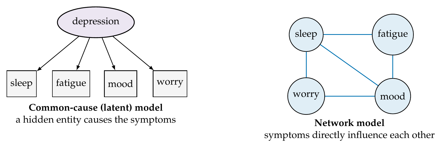
Note. The common-cause model (left) explains symptom correlations by a latent entity that causes each symptom; the network model (right) explains them by direct interactions among the symptoms. On cross-sectional data the two are statistically near-equivalent, so the choice is partly interpretive; intensive longitudinal data constrain the dynamics but do not fully settle the question.
Honesty requires meeting the equivalence problem at the outset. On cross-sectional data a network model and a latent-variable model can be statistically near-equivalent, fitting the same covariance matrix equally well, so that the data alone cannot adjudicate between a hidden common cause and a web of direct interactions (Marsman et al., 2018; van der Maas et al., 2006). This is not a fatal objection to networks, but it is a boundary on their claims: a well-fitting network is a representation of the covariance structure, not a demonstrated mechanism. Intensive longitudinal data help, because the temporal ordering of a dynamic network constrains which stories are viable in ways a single snapshot cannot, but they do not settle the matter, since the interval and confounding cautions of Chapters 25 and 27 apply to temporal edges verbatim. The book’s stance is that networks are a powerful representational and hypothesis-generating framework whose inferential claims must be earned, and the rest of the chapter is about the earning.
28.2 Estimating Networks
The workhorse model is the Gaussian graphical model, and its defining move is partialling. A correlation network draws an edge between every pair of variables that covary, and because almost everything in psychology covaries, such a network is a dense, uninformative web. The Gaussian graphical model instead draws an edge between two variables only if they are associated after conditioning on all the others, a partial correlation, so that an association that runs entirely through a third variable disappears and only direct, conditional associations remain. Figure 28.2 shows the contrast on the symptom_net data: the correlation network wires nearly everything together, while the partial-correlation network keeps a sparse backbone of direct edges. The partial correlations are read off the inverse of the covariance matrix, the precision matrix, whose off-diagonal zeros are precisely the absent edges, a fact the foundations box records. An edge in this network is a conditional association and nothing more, not a causal path, a point the pitfalls box returns to.
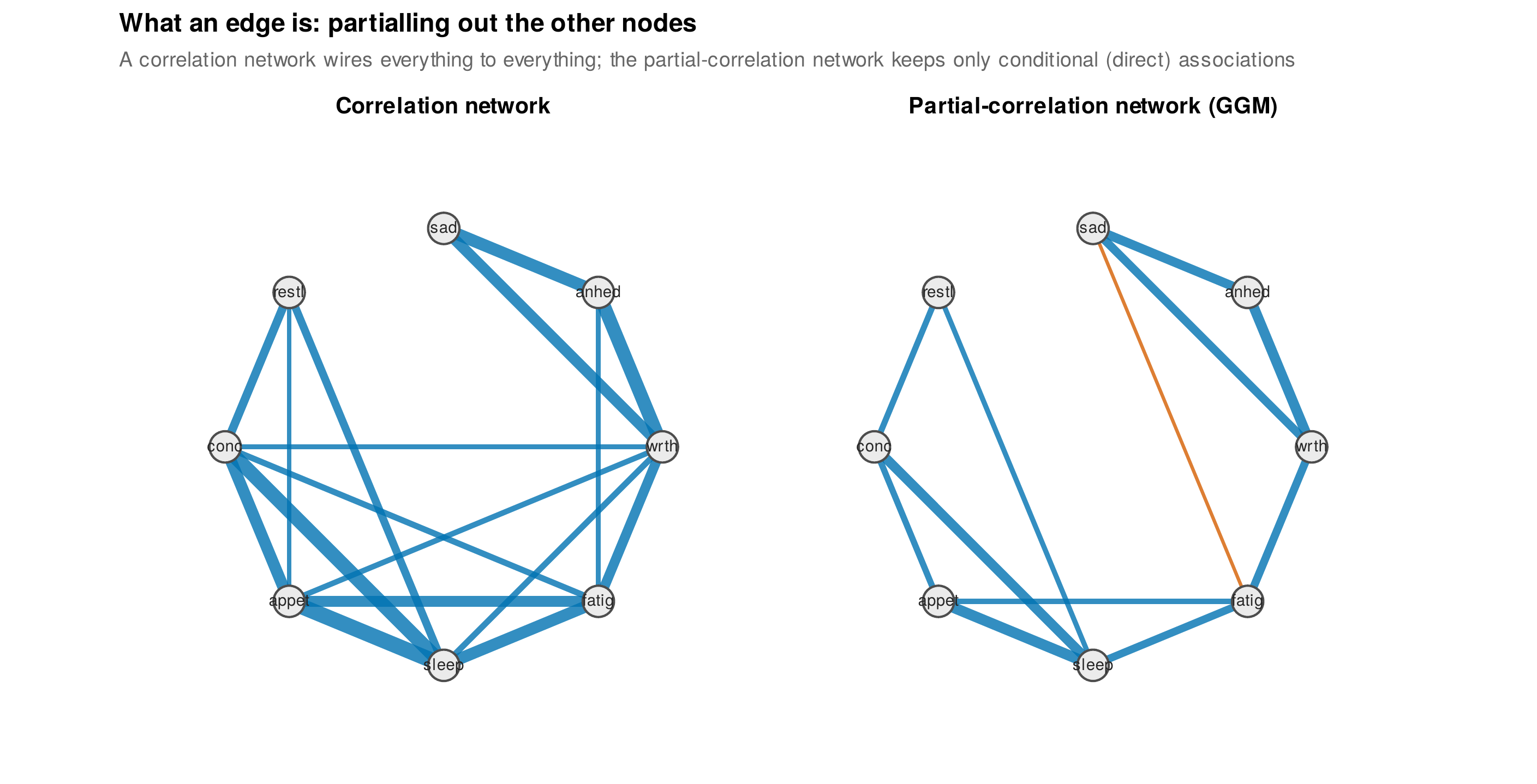
Note. Left: a correlation network on symptom_net, dense because indirect associations are drawn as edges. Right: the partial-correlation network (Gaussian graphical model), sparse because only conditional, direct associations survive. Blue edges are positive, red negative; width is the partial correlation’s magnitude.
Because a sample partial correlation is never exactly zero, estimation needs a principle for deciding which small edges are real, and the standard answer is regularization. The graphical lasso, and the nodewise-regression approach used here, shrink small partial correlations to exactly zero, producing a sparse network, and the amount of shrinkage is set by a tuning penalty chosen to optimize an extended Bayesian information criterion (Epskamp & Fried, 2018). Figure 28.3 shows the regularization path, the number of edges falling as the penalty rises, with the criterion selecting a penalty that here recovers close to the true number of edges. Regularization is not free: it trades false positives against false negatives, and a regularized zero is an absence of evidence for an edge, not evidence of its absence, so the method’s recent literature has debated when nonregularized estimation with explicit model selection is preferable (Williams et al., 2019; Isvoranu & Epskamp, 2023). Table 28.2 lays out the estimation choices, and the software note flags that this area moved after 2020 and should be checked at analysis time.
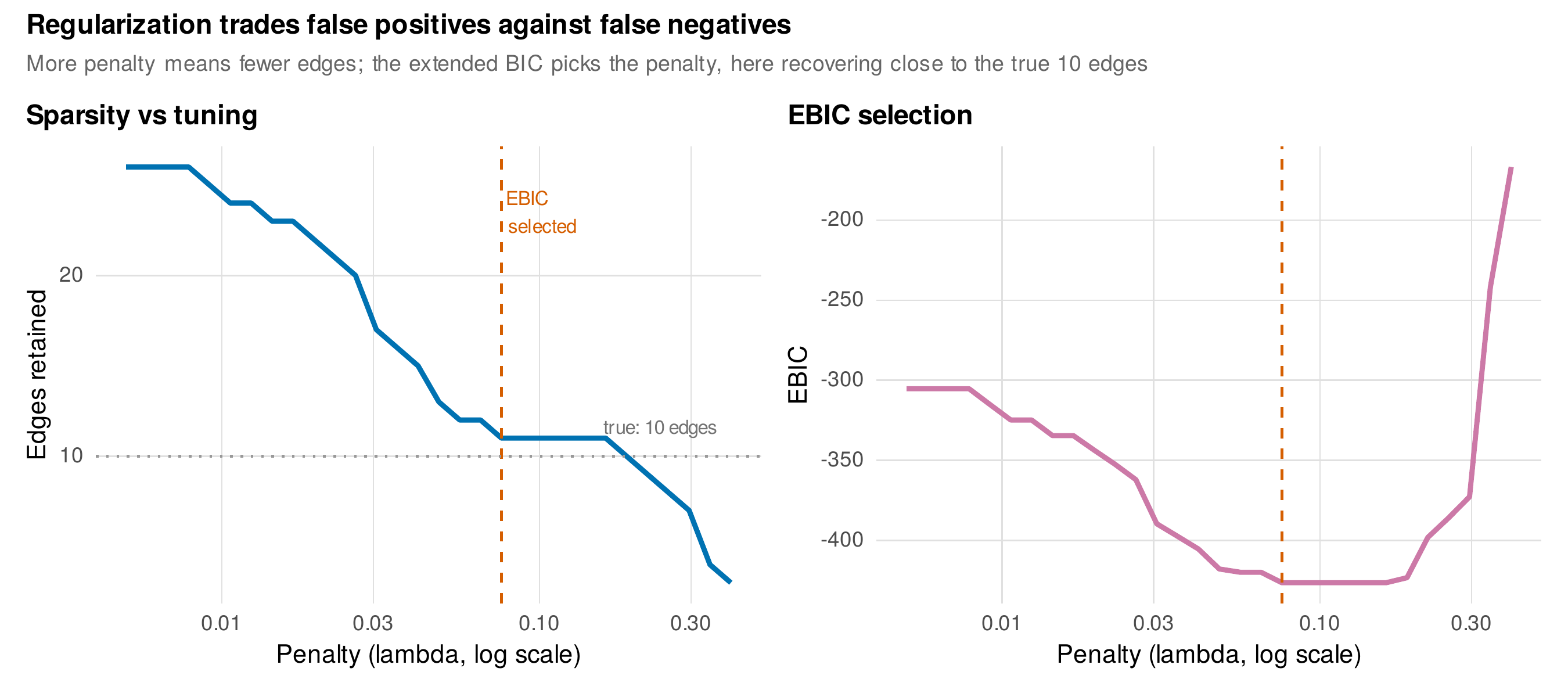
Note. The number of retained edges (left) falls as the penalty grows; the extended Bayesian information criterion (right) selects a penalty, here recovering close to the true ten edges. A regularized zero means an edge was not selected, not that it is known to be absent.
The intensive-longitudinal case produces not one network but three, and keeping them distinct with their matrices of origin is the chapter’s rule. Estimating a multilevel vector autoregression on affect_ema, exactly the model of Chapter 25, yields the triptych of Figure 28.4: a temporal network whose directed edges are the lagged cross-effects, the off-diagonals of the transition matrix; a contemporaneous network whose undirected edges are the partial correlations of the within-person innovations; and a between-person network whose edges are the partial correlations of the person means. These are the same objects Chapter 25 estimated as matrices, now wearing network clothing, and Table 28.1 is the Rosetta that maps the two vocabularies. The rule that every network figure must state its matrix of origin is not pedantry; a reader shown an undirected network without being told whether it is contemporaneous or between-person cannot know what within-person or between-person claim it licenses.
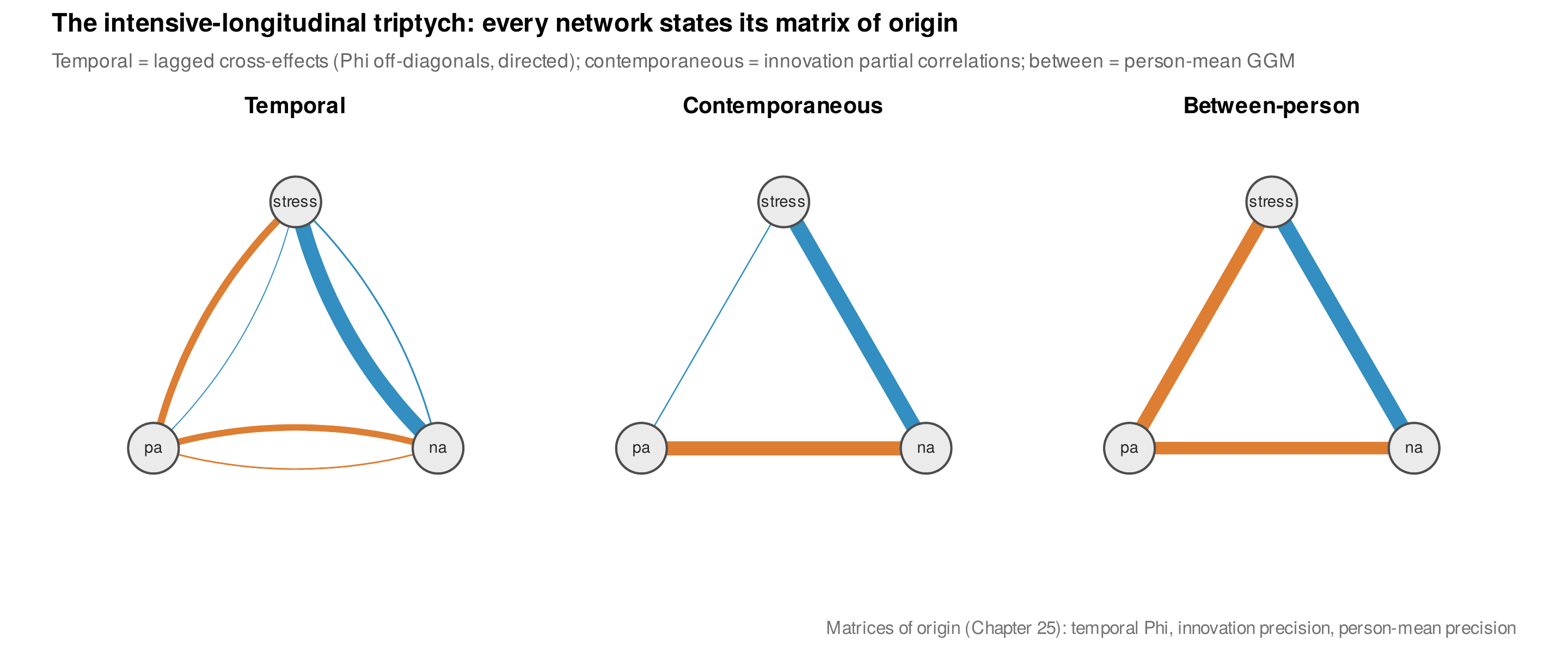
Note. From a multilevel vector autoregression on affect_ema: the temporal network (directed lagged cross-effects, the transition matrix off-diagonals), the contemporaneous network (innovation partial correlations), and the between-person network (person-mean partial correlations). These are Chapter 25’s three matrices as networks; every network figure must name its matrix of origin.
Table 28.1. Network objects and their Chapter 25 matrices (the Rosetta).
| Network (this chapter) | Matrix (Chapter 25) | Edge meaning |
|---|---|---|
| Temporal network | Transition matrix \(\boldsymbol{\Phi}\) off-diagonals | Directed lagged cross-effect (partialled) |
| Contemporaneous network | Innovation precision matrix | Same-occasion conditional association |
| Between-person network | Person-mean precision matrix | Between-person conditional association |
| Cross-sectional GGM | Precision matrix of the data | Conditional association at one occasion |
Note. One set of objects, two vocabularies. The network is a display of a precision or transition matrix; its edges inherit exactly the meaning and the cautions of the matrix that generated it, including the interval-dependence of temporal edges (Chapter 27).
Foundations Box • Partial correlations, the precision matrix, and the EBIC
For multivariate normal data with covariance \(\boldsymbol{\Sigma}\), the precision matrix is \(\mathbf{K} = \boldsymbol{\Sigma}^{-1}\), and the partial correlation between variables \(i\) and \(j\) controlling for all others is \(\rho_{ij\cdot} = -k_{ij}/\sqrt{k_{ii}k_{jj}}\). The Gaussian graphical model is exactly the pattern of nonzero off-diagonals of \(\mathbf{K}\): a zero there means \(i\) and \(j\) are conditionally independent given the rest, which is the absence of an edge. Estimation by the graphical lasso maximizes the Gaussian log-likelihood penalized by \(\lambda \sum_{i\neq j}|k_{ij}|\), which shrinks small entries to exactly zero; nodewise regression achieves the same sparsity by lasso-regressing each variable on the rest and keeping an edge when both directions survive. The penalty \(\lambda\) is chosen to minimize the extended Bayesian information criterion, \(\mathrm{EBIC} = -2\ell + E\log n + 4\gamma E \log p\), where \(\ell\) is the log-likelihood, \(E\) the number of edges, \(p\) the number of nodes, and \(\gamma\) a hyperparameter (commonly \(0.5\)) that adds an extra penalty for density, making the criterion conservative in the many-node, modest-\(n\) regime psychology inhabits.
The estimation is licensed by the exhibit that is this chapter’s distinctive contribution: the truth audit. Because symptom_net is generated from a known sparse network, the estimate can be scored against the truth, and Figure 28.5 does so. The estimated network recovers all ten true edges, a sensitivity of \(1.00\), with a specificity of \(0.94\) and a couple of false-positive edges, and the estimated and true edge weights correlate at \(0.95\). The message is precise and it is neither triumphant nor defeatist: at a realistic sample size the regularized estimator recovers the true structure well but not perfectly, capturing every real edge while admitting a few spurious ones, so a published network should be read as a good but imperfect estimate of a structure, not as the structure itself. This honesty is the price of the vividness, and the run-it-in-R panel shows the whole estimation and audit.
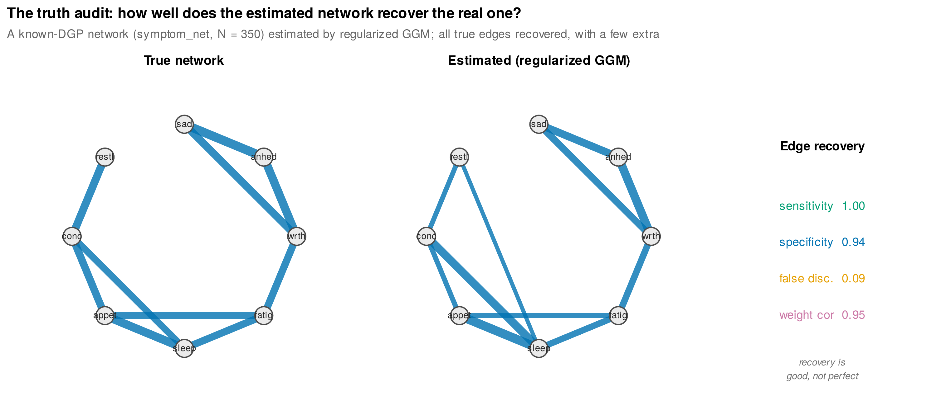
Note. A network generated from a known sparse structure (symptom_net, \(N=350\)) estimated by regularized Gaussian graphical modeling. All ten true edges are recovered (sensitivity \(1.00\)) with a specificity of \(0.94\) and a weight correlation of \(0.95\). Recovery is good, not perfect, the honest reading of any estimated network.
# Estimate a regularized GGM and audit it against the known truth
sn <- readRDS("Examples/data/symptom_net.rds"); tr <- attr(sn, "truth")
X  <- as.matrix(sn[sn$group == 1, tr$nodes])
pcor <- function(X){ P <- -cov2cor(solve(cov(X))); diag(P) <- 0; P }   # partial correlations
reg  <- regularized_ggm(X)          # nodewise lasso (glmnet) + EBIC selection (ch28_analysis)
# audit: which true edges did we recover?
ut <- upper.tri(tr$pcor)
sensitivity <- sum((reg$W != 0)[ut] &  (tr$pcor != 0)[ut]) / sum((tr$pcor != 0)[ut])  # 1.00
specificity <- sum((reg$W == 0)[ut] &  (tr$pcor == 0)[ut]) / sum((tr$pcor == 0)[ut])  # 0.94
cor(reg$W[ut], tr$pcor[ut])          # 0.95: estimated vs true edge weights
Table 28.2. Network estimation choices.
| Choice | Options | Guidance |
|---|---|---|
| Edge definition | Correlation vs partial correlation | Partial correlation (GGM); correlations wire in indirect links |
| Sparsity | Regularized (glasso/EBIC) vs nonregularized with model search | Regularized is the default; nonregularized alternatives debated (verify current guidance) |
| ILD structure | Nodewise (mlVAR) vs joint (graphicalVAR, DSEM) | Nodewise is fast; joint respects the full likelihood |
| Random effects | Orthogonal vs correlated | Correlated is more realistic but costlier; the Chapter 25 caveats apply |
| Node set | All items vs redundancy-pruned | Prune near-duplicate nodes first (Section 28.4) |
Note. The estimation literature moved substantially after 2020; the regularized-versus-nonregularized debate in particular should be checked at analysis time. Whatever the choice, report it, and audit against simulation when the stakes are high.
28.3 Stability, Accuracy, and Replicability
A network estimated once is a point estimate, and its edges and centrality summaries carry uncertainty that a single layout hides. The accuracy-and-stability toolkit makes that uncertainty visible (Epskamp et al., 2018). Figure 28.6 shows two of its outputs. A nonparametric bootstrap, resampling persons and re-estimating, produces a confidence interval for each edge weight, and edges whose intervals cross zero are not reliably distinguishable from absent. A case-dropping bootstrap, re-estimating on progressively smaller subsamples, tracks how well the centrality ordering is preserved, summarized by a centrality-stability coefficient, the largest proportion of cases that can be dropped while the strength ordering still correlates above \(0.7\) with the full-sample ordering in most subsamples; here that coefficient is \(0.45\), moderate, meaning the ordering is not rock-solid. The threshold conventions are in Table 28.3.
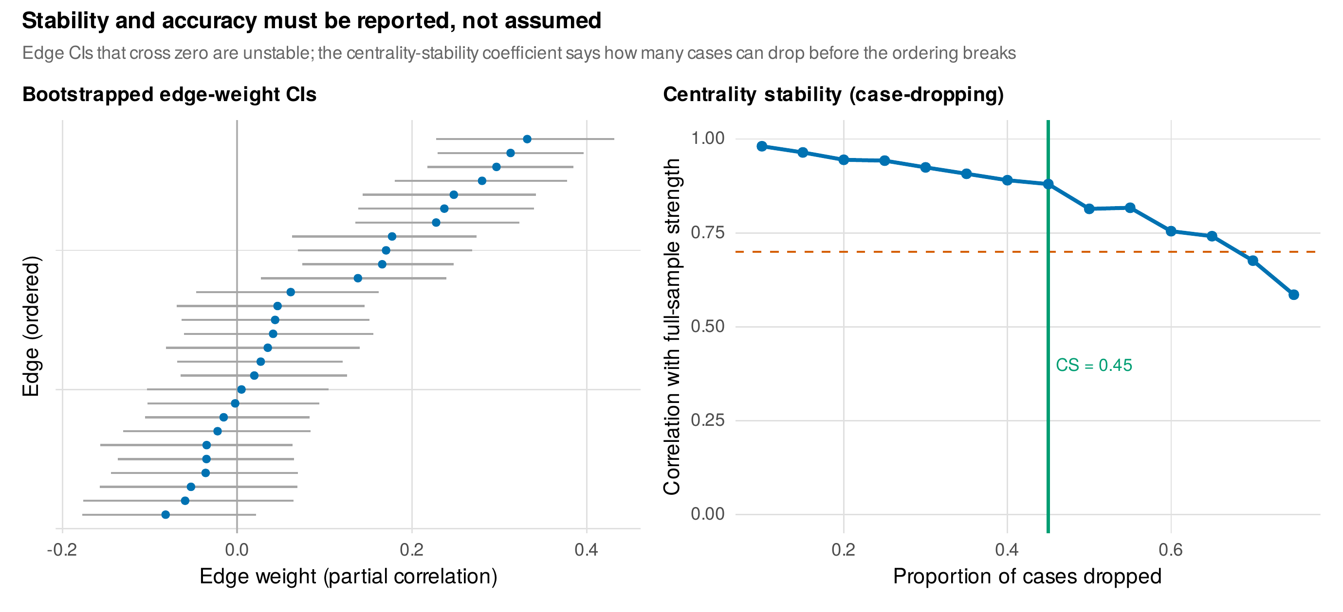
Note. Left: bootstrapped edge-weight confidence intervals; edges whose intervals cross zero are unstable. Right: the case-dropping centrality-stability curve, with the coefficient marking how many cases can drop before the strength ordering degrades (\(0.45\) here). These diagnostics are mandatory, not optional.
The replicability of psychological networks became a public controversy, and the chapter treats it as content. The critical claim was that symptom networks estimated on different samples of the same population can differ substantially, casting doubt on their reliability (Forbes et al., 2017), and the reply argued that the comparison metrics were themselves flawed and that networks replicate better than the critique implied (Borsboom et al., 2017). The resolution the field has reached is that different aspects replicate differently: the presence of the strong edges replicates well, exact edge weights less so, and the ordering of centrality, especially the identity of the single most central node, least of all. Figure 28.7 demonstrates this on two random halves of the same sample: the edge weights correlate at \(0.60\) and the strength ordering at \(0.78\), respectable, yet the single most central node differs between the halves, from one symptom to another. The practical lesson is to report what replicates, the strong edges and the coarse structure, and to resist the temptation to build a story on the most central node when that node is precisely the least stable feature. The pitfalls box collects the ways a network analysis oversells.
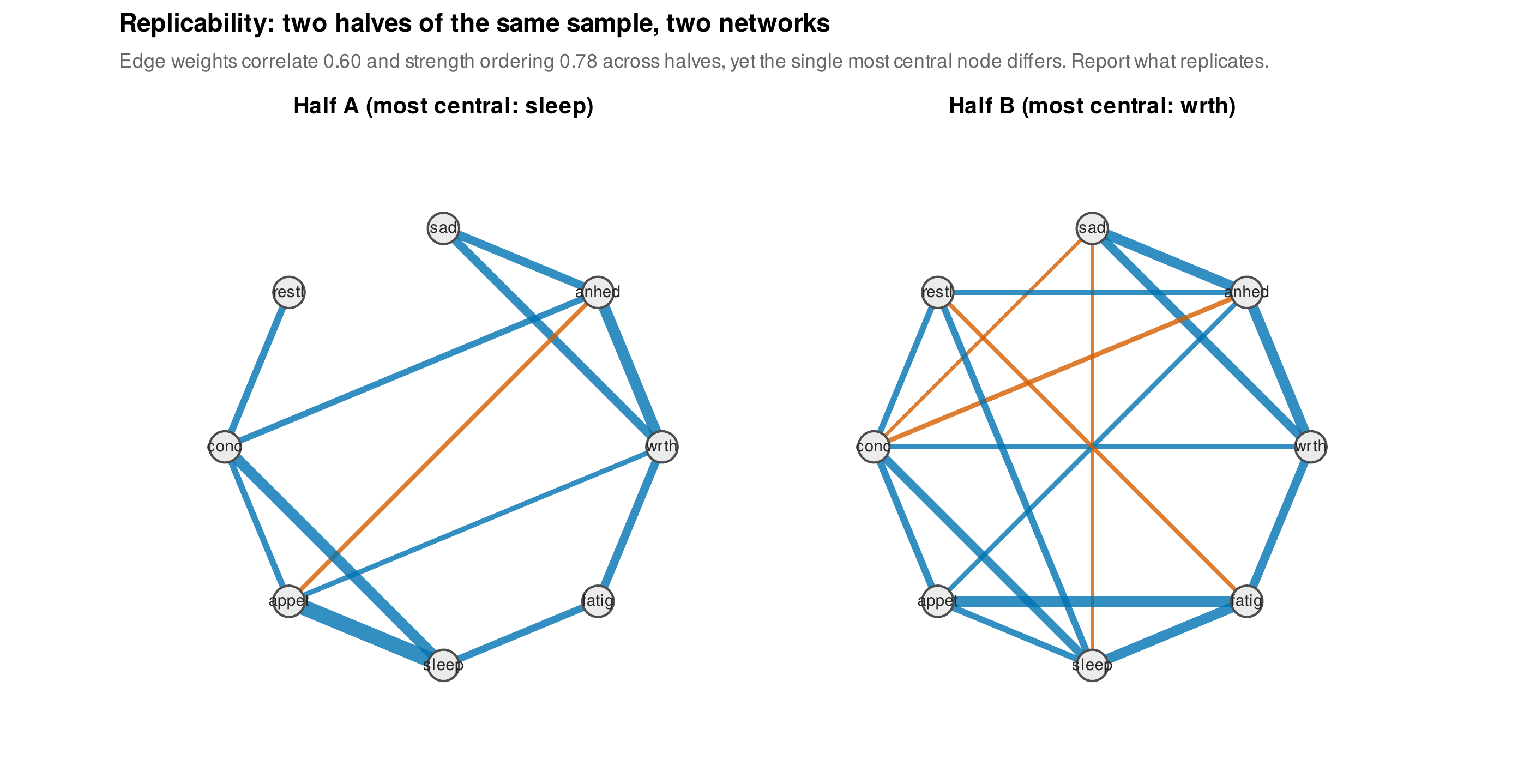
Note. Networks estimated on two random halves of symptom_net. Edge weights correlate at \(0.60\) and strength ordering at \(0.78\), yet the single most central node differs between the halves. Strong edges and coarse structure replicate; the most central node often does not.
Table 28.3. Stability metrics and their thresholds.
| Metric | What it assesses | Rule of thumb |
|---|---|---|
| Bootstrapped edge CI | Edge-weight uncertainty | Interval crossing zero: edge not reliable |
| Edge-weight difference test | Whether two edges differ | Wide overlap: do not rank edges |
| Centrality-stability (CS) | Preservation of centrality ordering | \(>0.5\) preferred, \(>0.25\) minimum |
| Centrality-difference test | Whether two nodes differ in centrality | Usually underpowered; interpret cautiously |
Note. The CS-coefficient is the largest proportion of cases droppable while the ordering still correlates above \(0.7\) with the full-sample ordering in \(95\%\) of subsamples. Values below \(0.25\) mean centrality should not be interpreted at all.
Common Pitfall • Four ways a network analysis oversells
First, reading an edge as a causal effect: an edge is a conditional association, and turning it into a causal arrow requires assumptions, no unmeasured confounders, correct causal direction, that the estimator does not supply and the design usually cannot support. Second, comparing two networks by eyeballing their layouts, when layout algorithms place nodes by force-directed heuristics that can move dramatically under tiny changes in the data, so that two networks with nearly identical weights can look different and two with different weights can look alike; compare the weight matrices, not the pictures. Third, driving a clinical claim from centrality, asserting that the most central symptom is the treatment target, when that inference needs causal edges, intervenability, and the absence of confounding, and when the central node is often the least stable feature of the estimate. Fourth, reading a regularized zero as evidence of absence, when it is only the absence of enough evidence to overcome the penalty, so a missing edge is not a demonstrated conditional independence.
28.4 Centrality and Its Discontents
Centrality indices rank nodes by their position in the network, and their use in psychology has outrun their justification. The most defensible index is strength, the sum of a node’s absolute edge weights, which is a transparent summary of how strongly a node is connected. The flow-based indices imported from social-network analysis, betweenness and closeness, assume that something travels along shortest paths through the network, an assumption that has no clear meaning for a partial-correlation network and that the critical literature has shown to be unreliable in psychological applications (Bringmann et al., 2019). Even strength is not importance in any causal sense without further assumptions (Dablander & Hinne, 2019), and it is vulnerable to a specific artifact that Figure 28.8 demonstrates: when two nodes are near-duplicates, redundant items measuring almost the same thing, each inflates the other’s centrality, because their shared variance is counted as connection. Adding a near-copy of one symptom raises that symptom’s strength from \(0.93\) to \(1.45\) and makes both twins look central, a topological artifact of redundancy rather than a substantive finding. The remedy is to prune redundant nodes before estimating, and the practice box gives the checks. Table 28.4 scopes the indices to their defensible uses.
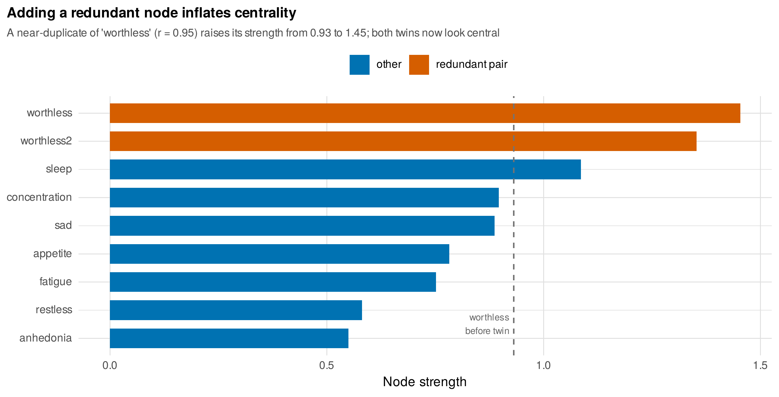
Note. A near-duplicate of the symptom “worthless” (correlation \(0.95\) with it) is added to symptom_net. Its strength jumps from \(0.93\) to \(1.45\), and both twins now appear central. Redundant nodes manufacture centrality; prune them before interpreting.
Table 28.4. Centrality indices: definition, assumption, and standing.
| Index | Definition | Standing in psychological networks |
|---|---|---|
| Strength | Sum of absolute edge weights | The most defensible; still not causal importance; inflated by redundancy |
| Expected influence | Signed sum of edge weights | Preferred over strength when edges have mixed signs |
| Betweenness | Shortest paths through a node | Assumption of flow along shortest paths is dubious; unstable |
| Closeness | Inverse total distance to others | Same flow assumption; rarely defensible |
| Bridge strength | Connection across communities | Useful for comorbidity questions, with the same cautions |
Note. Report strength or expected influence, prune redundant nodes first, and treat betweenness and closeness with skepticism. No centrality index establishes a treatment target without a causal argument the network alone cannot provide.
The clinical aspiration, that a central symptom is the best point to intervene, deserves its argument stated in full, because it is a good hypothesis and a bad conclusion. To move from centrality to a treatment target requires that the edges be causal rather than merely associational, that the central node be something one can actually intervene on, and that no confounder be inflating both its centrality and its apparent influence. None of these follows from the estimated network, so the honest status of a central symptom is a testable hypothesis to be examined with intervention-informed designs, not a conclusion to be acted on. Framed that way, centrality is a legitimate engine of hypotheses, which is a real contribution, provided the hypotheses are labeled as such.
28.5 Person-Specific Structure: GIMME
The networks so far describe a sample, but the heterogeneity that Chapter 25 documented means that different people may have qualitatively different structures, not just different parameter values, and when the structure itself is the question a different method is needed. Group iterative multiple model estimation, GIMME, discovers person-specific directed networks while detecting the paths that are shared across the sample (Gates & Molenaar, 2012; Beltz & Gates, 2017). Its logic is a search: it builds each person’s network by adding the lagged and contemporaneous directed edges that most improve fit, and it designates an edge as group-level when it appears in a large majority of individuals, so that the output separates a shared skeleton from individual embellishments, with an optional middle layer of subgroups. Figure 28.9 shows the idea on simulated data with a planted structure: a group path that all persons share, here the analogue of stress driving negative affect, recurs in nearly everyone and is correctly flagged as group-level, while a path planted only in a subgroup appears in just those individuals and is correctly left as person-specific. The distinction from the multilevel and dynamic-structural-equation models of Chapter 25 is exactly this: those models estimate a common structure with varying parameters, while GIMME searches for the structure itself person by person, so it is the tool when qualitative structural heterogeneity, rather than parameter heterogeneity, is the object of study. Table 28.5 draws the selection guide, and the practice box notes GIMME’s search-based nature and its replication needs.
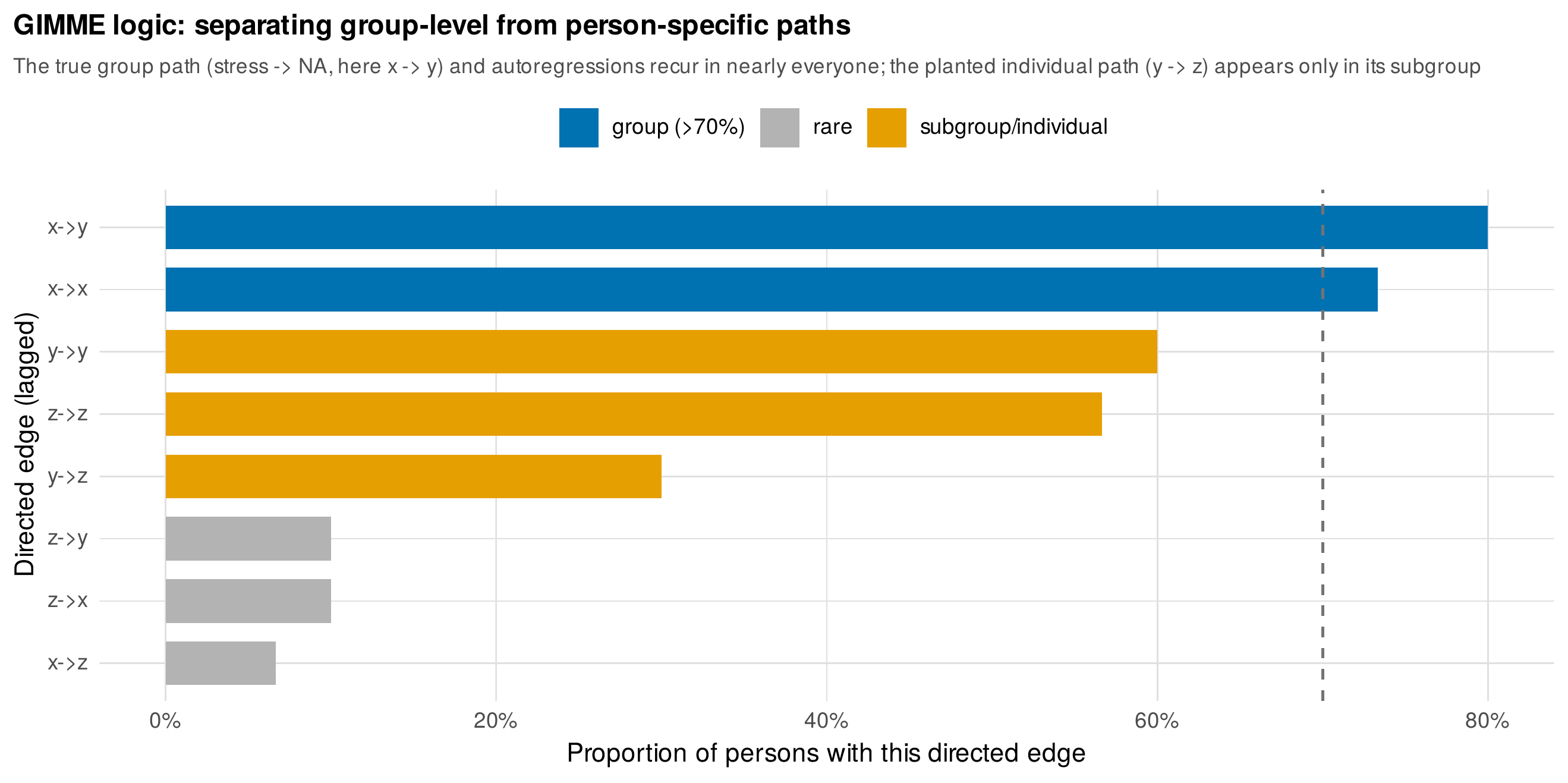
Note. The proportion of persons showing each directed lagged edge in simulated data. The planted group path and the autoregressions recur in most persons and are flagged group-level (above the dashed threshold); the path planted only in a subgroup appears in just those individuals. GIMME searches for the structure, not just its parameters.
Table 28.5. Choosing among person-specific dynamic methods.
| Method | What varies across persons | Use when |
|---|---|---|
| Multilevel VAR (Ch 25) | Parameters, shared structure | The structure is common; you want average dynamics and their spread |
| DSEM (Ch 25) | Parameters, with latent centering | Same, plus measurement and latent decomposition |
| GIMME | Structure itself (which edges exist) | Qualitative heterogeneity; different people, different maps |
Note. When people share a structure and differ in degree, the multilevel and dynamic-structural-equation models are right; when people differ in which connections exist at all, GIMME’s structure search is the tool. Its individual paths are search results needing replication, not established causal maps.
In Practice • Node selection and the search-based nature of GIMME
Before estimating any network, prune the node set for redundancy: two items that are near-paraphrases will manufacture a spurious strong edge and inflate each other’s centrality, so check inter-item correlations and content overlap and collapse or drop near-duplicates first. Attend to missing data, because listwise deletion can distort a network estimated from partial correlations and the intensive-longitudinal missingness of Chapter 6 needs a principled handling. And treat GIMME’s output with the humility its method demands: because it builds structure by a data-driven search over possible edges, its individual-level paths are hypotheses discovered in the data, vulnerable to the same overfitting as any stepwise search, so they require replication in fresh data before they are read as a person’s causal architecture, and the group-level paths, resting on a majority across persons, are the more trustworthy part of the output.
28.6 Comparing Networks and the Claims Ladder
Research questions often ask whether two networks differ, before and after therapy, between diagnostic groups, and the honest test is a permutation test rather than an eyeball comparison of layouts. The network comparison test permutes the group labels to build a null distribution for a chosen difference statistic, the difference in global connectivity, in a specific edge, or in overall structure, and compares the observed difference against it (van Borkulo et al., 2023). Figure 28.10 applies it to the two groups of symptom_net, which were generated to differ in exactly one edge: the test correctly finds no difference in global connectivity, a permutation \(p\) of \(0.33\), while detecting the planted edge difference, \(p=0.005\), which is the right pattern, a localized difference that a global statistic would miss. The test’s power is limited at realistic sample sizes, so a null result is weak evidence of equivalence rather than proof of it, and the comparison of networks over time connects forward to the time-varying networks of Chapter 32.
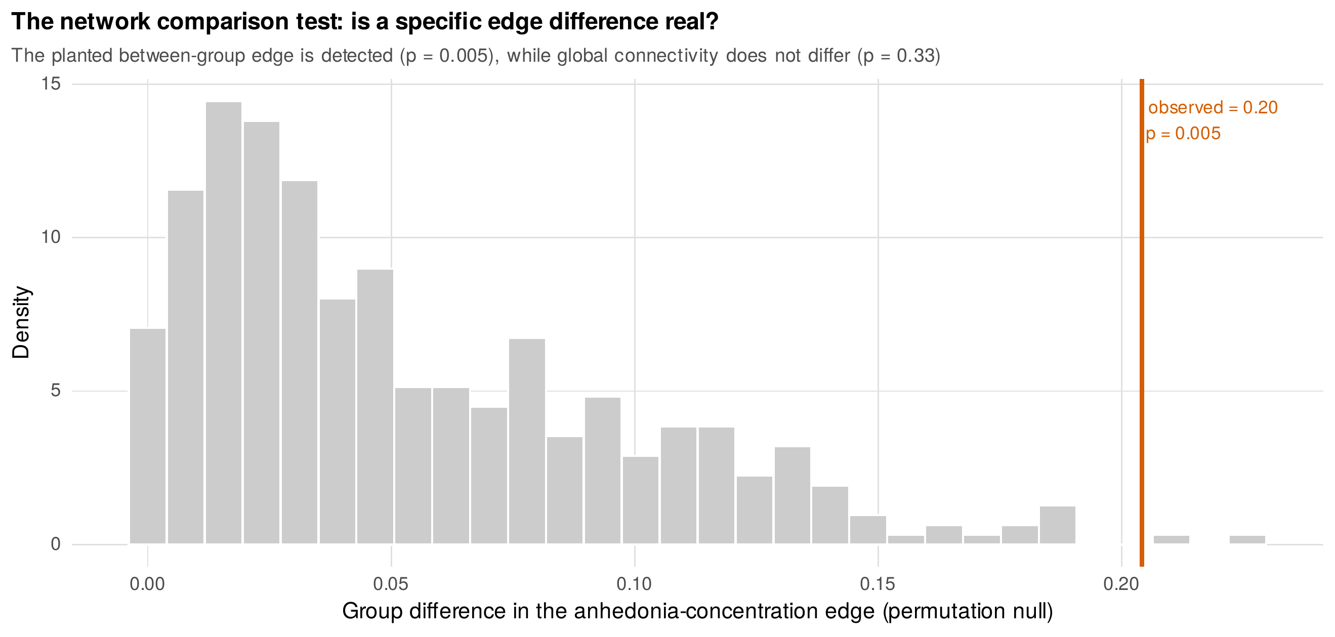
Note. A permutation test on the two groups of symptom_net, generated to differ in one edge. The planted edge difference is detected (\(p=0.005\), red line against the permutation null), while global connectivity does not differ (\(p=0.33\)). Permutation tests localize differences that global summaries miss, with power limited at psychological sample sizes.
The chapter closes by fixing the language of network claims to the evidence, because the recurring failure of the literature has been to describe a conditional-association structure as though it were a discovered causal mechanism. Figure 28.11 draws a claims ladder with four rungs. The lowest is description: the network displays the pattern of conditional associations in this sample, a claim the estimate supports directly. The second is conditional-association structure: these variables are directly associated after controlling for the others, a claim that adds the partialling logic and requires the stability checks. The third is predictive dynamics: in the temporal network, one variable’s earlier state forecasts another’s later state, a claim that requires longitudinal data and inherits the interval cautions of Chapter 27. The highest is causal system: the variables causally influence one another in the way the edges depict, a claim that requires assumptions or interventions the network alone cannot provide, and that most network studies have not earned. Table 28.6 pairs each rung with a reporting checklist and a language template, so that a results section can be written at the rung its evidence reaches and no higher. This ladder aligns with the estimand ladders of Chapters 21 and 25, and it is the chapter’s final discipline: the machinery is powerful, and the claims must be earned.
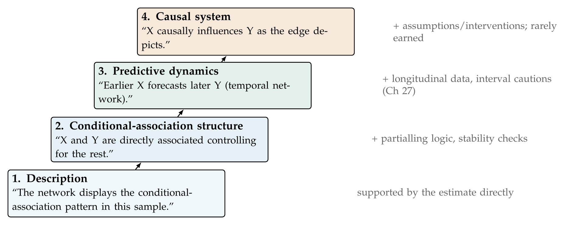
Note. Each rung is a stronger claim requiring more than the last. The estimate supports description directly; conditional-association structure adds the partialling logic and stability; predictive dynamics adds longitudinal data and the interval cautions of Chapter 27; a causal-system claim requires assumptions or interventions the network alone cannot supply. Write at the rung the evidence reaches.
Writing up a network analysis means reporting the estimation, the stability, and the claims at their earned rung. The report should state the node set and any redundancy pruning, the estimation method and its tuning, and whether the network is cross-sectional or one panel of the intensive-longitudinal triptych with its matrix of origin. It should present the accuracy and stability diagnostics, the edge-weight intervals and the centrality-stability coefficient, and it should temper centrality claims accordingly, reporting strength rather than the flow indices and treating a central node as a hypothesis. For a group comparison it should give the permutation test with its power caveat. And throughout it should keep the language on the ladder: an edge is a conditional association, a temporal edge is a prediction with interval caveats, and a causal claim is made only with the design that earns it. A model sentence reads: “A regularized partial-correlation network was estimated (extended BIC, \(\gamma=0.5\)) after pruning two near-redundant items; the strongest edges (worthlessness with sadness and with anhedonia) were stable across bootstrapped intervals, while the centrality-stability coefficient for strength was \(0.45\), so centrality is reported descriptively and the most central node is not interpreted as a treatment target.”
Software Note • The network software ecosystem
The standard toolchain is an R ecosystem: qgraph for estimation and display, bootnet for the accuracy and stability workflows, mlVAR and graphicalVAR for the intensive-longitudinal triptych, psychonetrics for a unified confirmatory framework, gimme for person-specific structure search, NetworkComparisonTest for group comparison, and mgm for mixed-type and time-varying networks. This ecosystem is actively maintained and its recommendations, especially on regularized versus nonregularized estimation, moved after 2020, so the current guidance should be checked at analysis time rather than taken from a textbook. The analyses in this chapter were built without these packages, which do not install in the present environment, using base R and glmnet for the nodewise regularized estimation, a hand-rolled partial-correlation and centrality toolkit, and hand-written bootstrap, permutation, and structure-search routines, so that each quantity, the truth-audit recovery, the stability coefficient, the redundancy inflation, could be checked against a known truth; the packages are the right choice for applied work.
Table 28.6. Network reporting checklist and claims-ladder templates.
| Element | What to report / language template |
|---|---|
| Node set | Items, redundancy pruning, and rationale |
| Estimation | Method, regularization and tuning, matrix of origin (if ILD) |
| Accuracy & stability | Edge-weight intervals; centrality-stability coefficient |
| Centrality | Strength or expected influence; treat as descriptive, not a target |
| Comparison | Permutation test with power caveat |
| Rung 1 (description) | “The network displays the conditional-association pattern in this sample.” |
| Rung 2 (structure) | “X and Y are directly associated controlling for the others.” |
| Rung 3 (dynamics) | “Earlier X predicts later Y” (temporal; interval caveats). |
| Rung 4 (causal) | Only with the assumptions or interventions that earn it. |
Note. Write the results section at the rung the evidence reaches. Most network studies are entitled to rungs one through three; the causal fourth rung requires a design the network alone does not provide.
Chapter Summary
The network approach represents psychological variables as a system of directly interacting components rather than the reflection of a latent common cause, a reframing that is generative for clinical and personality science but whose central object, the estimated network, invites overclaiming. On cross-sectional data the network and latent accounts are near-equivalent, so a network is a representation of covariance structure, not a demonstrated mechanism. The Gaussian graphical model draws an edge only where two variables are associated after conditioning on the rest, a partial correlation read from the precision matrix, and regularization shrinks small edges to zero under an information criterion, trading false positives against false negatives. The intensive-longitudinal triptych, temporal, contemporaneous, and between-person networks, is exactly Chapter 25’s three matrices in network clothing, and every network figure must name its matrix of origin. The truth audit, the chapter’s distinctive exhibit, shows on known-DGP data that a regularized estimator recovers a real structure well but not perfectly, capturing every true edge while admitting a few spurious ones, so a published network is a good estimate, not the truth. Accuracy and stability must be reported: bootstrapped edge intervals reveal which edges are reliable, and the centrality-stability coefficient reveals how firmly the centrality ordering holds, which on realistic data is only moderately. Replicability differs by aspect, strong edges and coarse structure replicate while the single most central node often does not, so centrality is reported descriptively, strength over the dubious flow indices, redundant nodes pruned to avoid manufactured centrality, and a central symptom is a hypothesis rather than a treatment target. GIMME searches for person-specific structure when qualitative heterogeneity is the question, separating shared paths from individual ones, and the network comparison test localizes group differences a global summary would miss. The chapter’s final discipline is the claims ladder, which fixes the language of a network result, description, conditional-association structure, predictive dynamics, causal system, to the evidence that supports it, so that the machinery is used at full strength and the claims are earned.
Beltz, A. M., & Gates, K. M. (2017). Network mapping with GIMME. Multivariate Behavioral Research, 52(6), 789–804. https://doi.org/10.1080/00273171.2017.1373014
Borsboom, D. (2017). A network theory of mental disorders. World Psychiatry, 16(1), 5–13. https://doi.org/10.1002/wps.20375
Borsboom, D., & Cramer, A. O. J. (2013). Network analysis: An integrative approach to the structure of psychopathology. Annual Review of Clinical Psychology, 9, 91–121. https://doi.org/10.1146/annurev-clinpsy-050212-185608
Borsboom, D., Fried, E. I., Epskamp, S., Waldorp, L. J., van Borkulo, C. D., van der Maas, H. L. J., & Cramer, A. O. J. (2017). False alarm? A comprehensive reanalysis of “Evidence that psychopathology symptom networks have limited replicability” by Forbes, Wright, Markon, and Krueger (2017). Journal of Abnormal Psychology, 126(7), 989–999. https://doi.org/10.1037/abn0000306
Bringmann, L. F., Elmer, T., Epskamp, S., Krause, R. W., Schoch, D., Wichers, M., Wigman, J. T. W., & Snippe, E. (2019). What do centrality measures measure in psychological networks? Journal of Abnormal Psychology, 128(8), 892–903. https://doi.org/10.1037/abn0000446
Bringmann, L. F., & Eronen, M. I. (2018). Don’t blame the model: Reconsidering the network approach to psychopathology. Psychological Review, 125(4), 606–615. https://doi.org/10.1037/rev0000108
Cramer, A. O. J., Waldorp, L. J., van der Maas, H. L. J., & Borsboom, D. (2010). Comorbidity: A network perspective. Behavioral and Brain Sciences, 33(2–3), 137–150. https://doi.org/10.1017/S0140525X09991567
Dablander, F., & Hinne, M. (2019). Node centrality measures are a poor substitute for causal inference. Scientific Reports, 9, Article 6846. https://doi.org/10.1038/s41598-019-43033-9
Epskamp, S. (2020). Psychometric network models from time-series and panel data. Psychometrika, 85(1), 206–231. https://doi.org/10.1007/s11336-020-09697-3
Epskamp, S., Borsboom, D., & Fried, E. I. (2018). Estimating psychological networks and their accuracy: A tutorial paper. Behavior Research Methods, 50(1), 195–212. https://doi.org/10.3758/s13428-017-0862-1
Epskamp, S., & Fried, E. I. (2018). A tutorial on regularized partial correlation networks. Psychological Methods, 23(4), 617–634. https://doi.org/10.1037/met0000167
Epskamp, S., Waldorp, L. J., Mõttus, R., & Borsboom, D. (2018). The Gaussian graphical model in cross-sectional and time-series data. Multivariate Behavioral Research, 53(4), 453–480. https://doi.org/10.1080/00273171.2018.1454823
Forbes, M. K., Wright, A. G. C., Markon, K. E., & Krueger, R. F. (2017). Evidence that psychopathology symptom networks have limited replicability. Journal of Abnormal Psychology, 126(7), 969–988. https://doi.org/10.1037/abn0000276
Fried, E. I., & Cramer, A. O. J. (2017). Moving forward: Challenges and directions for psychopathological network theory and methodology. Perspectives on Psychological Science, 12(6), 999–1020. https://doi.org/10.1177/1745691617705892
Gates, K. M., & Molenaar, P. C. M. (2012). Group search algorithm recovers effective connectivity maps for individuals in homogeneous and heterogeneous samples. NeuroImage, 63(1), 310–319. https://doi.org/10.1016/j.neuroimage.2012.06.026
Haslbeck, J. M. B., & Waldorp, L. J. (2020). mgm: Estimating time-varying mixed graphical models in high-dimensional data. Journal of Statistical Software, 93(8), 1–46. https://doi.org/10.18637/jss.v093.i08
Isvoranu, A.-M., & Epskamp, S. (2023). Which estimation method to choose in network psychometrics? Deriving guidelines for applied researchers. Psychological Methods, 28(4), 925–946. https://doi.org/10.1037/met0000439
Marsman, M., Borsboom, D., Kruis, J., Epskamp, S., van Bork, R., Waldorp, L. J., van der Maas, H. L. J., & Maris, G. (2018). An introduction to network psychometrics: Relating Ising network models to item response theory models. Multivariate Behavioral Research, 53(1), 15–35. https://doi.org/10.1080/00273171.2017.1379379
Robinaugh, D. J., Hoekstra, R. H. A., Toner, E. R., & Borsboom, D. (2020). The network approach to psychopathology: A review of the literature 2008–2018 and an agenda for future research. Psychological Medicine, 50(3), 353–366. https://doi.org/10.1017/S0033291719003404
van Borkulo, C. D., van Bork, R., Boschloo, L., Kossakowski, J. J., Tio, P., Schoevers, R. A., Borsboom, D., & Waldorp, L. J. (2023). Comparing network structures on three aspects: A permutation test. Psychological Methods, 28(6), 1273–1285. https://doi.org/10.1037/met0000476
van der Maas, H. L. J., Dolan, C. V., Grasman, R. P. P. P., Wicherts, J. M., Huizenga, H. M., & Raijmakers, M. E. J. (2006). A dynamical model of general intelligence: The positive manifold of intelligence by mutualism. Psychological Review, 113(4), 842–861. https://doi.org/10.1037/0033-295X.113.4.842
Williams, D. R., Rhemtulla, M., Wysocki, A. C., & Rast, P. (2019). On nonregularized estimation of psychological networks. Multivariate Behavioral Research, 54(5), 719–750. https://doi.org/10.1080/00273171.2019.1575716