Chapter 29
Survival and Event-History Analysis
The chapters to this point have modeled how a continuous attribute rises and falls over time. Many of the questions that motivate longitudinal research are not about a level at all but about a moment: when a patient relapses, when a student first fails a course, when a couple separates, when an employee quits, when an abstinent smoker lights the first cigarette. These are timing questions, and they defeat the machinery of the preceding chapters for a single stubborn reason. At the end of a study, some people have had the event and some have not, and for those who have not, the true event time is not missing in the ordinary sense but known to lie beyond the observation window. This is censoring, and a mean that discards the censored cases, or that pretends the last observation was the event, is not merely imprecise but biased, sometimes grossly. Survival analysis, also called event-history analysis, is the family of methods built to keep the censored cases in the analysis at their full informational worth, neither dropped nor fabricated. This chapter takes the psychologist’s road into that family. It begins with discrete-time survival, where the data become a person-period file and the model is the logistic regression of Chapter 15 wearing a new interpretation, because most psychological events are recorded in weeks or grades or waves rather than to the instant. It then develops the continuous-time apparatus, the Kaplan-Meier estimator and the Cox proportional-hazards model, with the discipline that their elegance demands, and it treats the errors that reviewers most often catch, immortal time, competing risks read off the wrong curve, and hazard ratios misread as risk ratios, as content to be mastered rather than footnotes. It closes by joining the survival submodel to the growth submodel of Chapters 13 and 14, so that outcome-dependent dropout, the missing-not-at-random mechanism promised in Chapter 6, is modeled rather than assumed away.
Learning Objectives
After working through this chapter, you should be able to: (1) define the survivor function, the hazard, and the cumulative hazard in both discrete and continuous time, and translate among them; (2) explain right, left, and interval censoring and state the noninformative-censoring assumption as the field’s silent relative of missing-at-random; (3) construct a person-period data set and fit a discrete-time hazard model as a logistic regression, choosing a baseline-hazard specification and reading covariate effects as hazard-odds ratios; (4) estimate and compare Kaplan-Meier curves with the log-rank test, and fit a Cox model with a defensible interpretation of the hazard ratio; (5) detect proportional-hazards violations with Schoenfeld residuals and resolve them with a time-varying coefficient; (6) incorporate time-varying covariates through counting-process data and recognize immortal-time bias; (7) extend to shared frailty, recurrent events, and competing risks, choosing cause-specific or subdistribution hazards by the question asked; (8) fit a shared-parameter joint longitudinal-survival model for outcome-dependent dropout; and (9) report a survival analysis to publication standard.
29.1 Timing Questions and the Survival Vocabulary
The fifth family of questions named in Chapter 1, questions about the occurrence and timing of events, has waited until now for its methods because those methods are unlike the others in the book. The object of inference is a duration, the time from a well-defined origin to a well-defined event, and the analytic difficulty is that at the close of data collection the duration is known exactly for some participants and only bounded for the rest. Consider the running example of this chapter, the relapse data, a simulated study of four hundred patients treated for a depressive episode and followed weekly for up to twenty-four weeks to observe whether and when symptoms return to a relapse threshold. The data are simulated from a known generating process so that every estimate can be audited against truth, a device this book uses throughout. By week twenty-four, one hundred eighty-one patients have relapsed, one hundred forty-eight have left care for reasons other than relapse, and seventy-one remain in remission and under observation. Only the first group has an observed relapse time. For the second and third, all that is known is that relapse, if it will occur at all, had not occurred by the moment observation ceased.
The temptation is to reach for a familiar summary, and each familiar summary fails in an instructive way. Averaging the relapse times of the one hundred eighty-one patients who relapsed yields a mean of about nine weeks, but this describes only the fast relapsers and silently discards more than half the sample, the very patients whose long times to relapse are the treatment’s success. Filling in each censored patient’s last observed week as though it were the relapse week yields a mean of about twelve weeks, an arbitrary number that would shrink if the study were shorter and grow if it were longer, tracking the design rather than the phenomenon. Regressing the observed follow-up time on treatment arm by ordinary least squares suggests that treated patients are followed about three and a half weeks longer, which conflates the benefit of treatment with the bookkeeping fact that patients who do not relapse are observed until the administrative end. The Kaplan-Meier estimator, which uses every patient for exactly as long as each is observed, places the median time to relapse at eighteen weeks, a figure none of the naive summaries recovers. Table 29.1 fixes the vocabulary that makes the correct analysis possible, and Figure 29.1 draws the censoring structure that the naive summaries mishandle.
Table 29.1. Survival Quantities in Discrete and Continuous Time
| Quantity | Continuous time | Discrete time (periods \(t=1,2,\dots\)) |
|---|---|---|
| Survivor \(S(t)\) | \(P(T>t)\), probability the event has not occurred by \(t\) | \(S(t)=\prod_{k\le t}\bigl(1-h(k)\bigr)\) |
| Hazard \(h(t)\) | \(\lim_{\Delta t\to 0}\dfrac{P(t\le T<t+\Delta t\mid T\ge t)}{\Delta t}\), an instantaneous rate | \(h(t)=P(T=t\mid T\ge t)\), a conditional probability in \([0,1]\) |
| Cumulative hazard | \(H(t)=\int_0^t h(u)\,du=-\log S(t)\) | \(H(t)=\sum_{k\le t} h(k)\) (approx.) |
| Median lifetime | smallest \(t\) with \(S(t)\le .5\) | smallest period with \(S(t)\le .5\) |
| Link to a model | \(h(t)=h_0(t)\exp(\mathbf{x}'\boldsymbol\beta)\) (Cox) | \(\mathrm{logit}\,h(t)=\alpha(t)+\mathbf{x}'\boldsymbol\beta\) (logistic) |
Note. The hazard is the central quantity because it is defined conditionally, among those still at risk, and so absorbs censoring naturally. In continuous time it is a rate that may exceed one; in discrete time it is a probability bounded by one. The survivor function is recovered from the hazard by accumulating survival period by period.
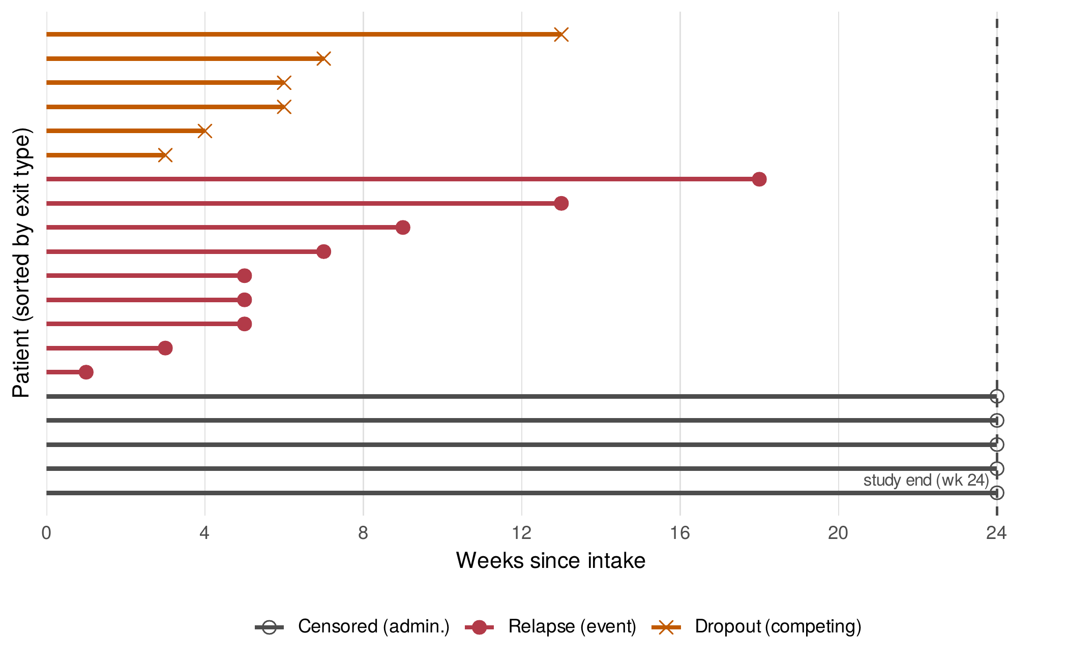
Note. Each horizontal strip is one patient’s follow-up from intake. A filled circle marks an observed relapse, the event of interest; a cross marks dropout, a different event that ends observation; an open circle at the dashed line marks a patient still in remission when the study closed at week twenty-four. The censored strips are not missing data to be discarded or imputed: each one records that the patient survived relapse-free for at least as long as the strip is drawn, information the hazard uses in full.
The conditional definition of the hazard is the conceptual pivot of the whole subject, and it is the definition students most often blur. The hazard at week \(t\) is not the probability that a randomly chosen patient relapses at week \(t\); it is the probability that a patient relapses at week \(t\) given that the patient had not relapsed before week \(t\). The risk set, the collection of those still event-free and under observation, shrinks over time as patients relapse, drop out, or reach the administrative boundary, and the hazard is always computed relative to the current risk set. This is exactly why censoring is tractable. A censored patient contributes to every risk set up to the moment of censoring and then simply leaves; nothing about that patient is fabricated, and nothing is thrown away. Figure 29.2 shows the hazard and the survivor function it implies for the relapse data, the two faces of the same distribution.
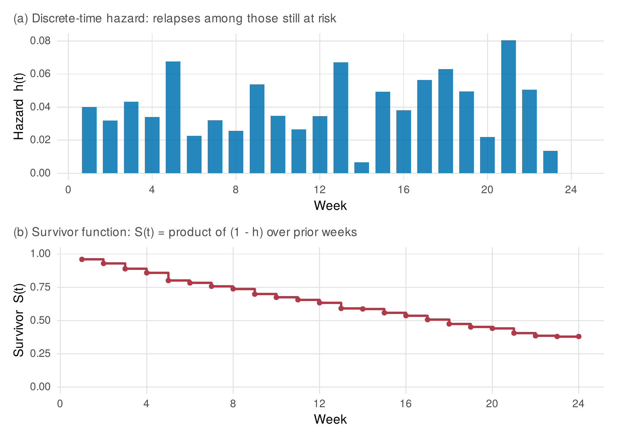
Note. Panel (a) is the empirical discrete-time hazard, the number of relapses in each week divided by the number of patients still at risk that week. Panel (b) is the survivor function obtained by accumulating relapse-free survival, \(S(t)=\prod_{k\le t}(1-h(k))\). A high hazard in a given week produces a steep drop in the survivor curve at that week; a hazard that rises and then falls produces a survivor curve that descends fastest in the middle of the study.
Censoring comes in kinds, and the kind matters. Right censoring, the case just described, occurs when the event has not happened by the end of observation, and it is by far the most common. Left censoring occurs when the event is known to have happened before observation began but its exact time is unknown, as when a survey finds that a respondent has already started smoking but cannot date the first cigarette. Interval censoring occurs when the event is known only to fall between two assessment waves, which is the true state of most panel data and which discrete-time methods handle gracefully. Across all kinds, the assumption that licenses the standard analysis is noninformative censoring: the mechanism that removes a patient from observation carries no information about that patient’s hazard beyond what the covariates already capture. This is the survival-analytic cousin of the missing-at-random assumption of Chapter 6, and it is just as untestable from the data at hand and just as consequential. If patients who are about to relapse are the ones who drop out, censoring is informative, the risk set is no longer representative of the patients the model imagines, and every estimate is biased in a direction that depends on the mechanism. The competing-dropout structure of the relapse data is built to be informative in exactly this way, and Section 29.6 confronts it directly rather than assuming it away.
Foundations Box • The likelihood with censoring
The reason censored cases can be retained without fabrication is visible in the likelihood. A patient observed to have the event at time \(t\) contributes the density of the event time there, which in the hazard parameterization is \(h(t)\,S(t^-)\): the patient survived up to \(t\) and then had the event. A patient right-censored at time \(c\) contributes only \(S(c)\): all that is known is survival past \(c\). Writing \(\delta_i=1\) for an observed event and \(\delta_i=0\) for censoring, the individual contribution is \(h(t_i)^{\delta_i}\,S(t_i)\), and in discrete time this factors period by period into a product of Bernoulli terms, one per period the patient is at risk, with “event” probability \(h(t)\). That factorization is the whole trick: it turns the person-period file into a set of independent Bernoulli trials and so turns survival estimation into logistic regression. The noninformative-censoring assumption is precisely what licenses treating \(S(c)\), rather than something depending on the reason for censoring, as the censored patient’s contribution.
29.2 Discrete-Time Survival: The Psychologist’s Entry
Most psychological events are not timed to the instant. Relapse is recorded at a weekly assessment, course failure at the end of a grading term, divorce at an annual wave. When the metric of time is coarse, discrete-time survival is not an approximation to be apologized for but the natural model, and its great pedagogical virtue is that it reduces to tools already in hand. The method, developed for psychology and education by Singer and Willett (1991, 1993) and by Allison (1982), rests on a single reshaping of the data. The person-period file expands each participant into one row per period the participant is at risk, from the first period through the period of the event or of censoring, with a binary indicator that equals one only in the period the event occurs. A patient who relapses in week five contributes five rows, the indicator zero in weeks one through four and one in week five. A patient censored at week twelve contributes twelve rows, the indicator zero throughout. Figure 29.3 draws the transformation, and the software note gives the few lines of R that perform it.
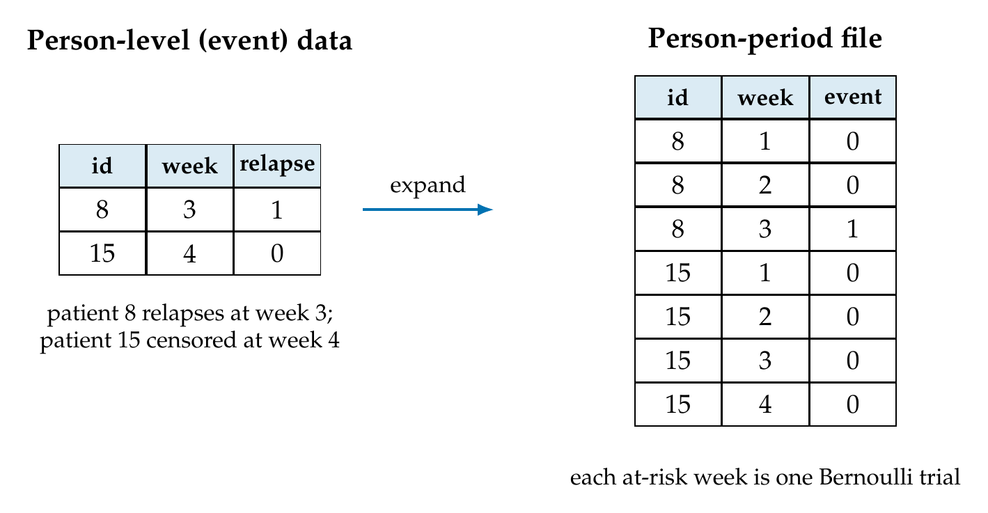
Note. The person-level table on the left holds one row per patient with the event time and an event indicator. The person-period file on the right holds one row per patient per at-risk week, with the event indicator equal to one only in the week the event occurs and zero otherwise. Censored patients contribute all-zero rows up to their censoring week. The expanded file is analyzed as a set of independent binary outcomes, which is why a logistic regression on it estimates the discrete-time hazard.
Software Note • Building and fitting the person-period file
# Expand person-level (time, status) to person-period, then fit the hazard.
build_pp <- function(df) do.call(rbind, lapply(seq_len(nrow(df)), function(i){
  k <- df$time[i]
  data.frame(person = df$person[i], week = 1:k,
             event = as.integer(df$status[i] == 1 & (1:k) == k)) }))
pp <- build_pp(relapse)                    # reproduces the shipped relapse_pp
# Discrete-time hazard model: baseline hazard + covariates (logit link)
m <- glm(event ~ ns(week, df = 4) + arm + severity, data = pp, family = binomial)
# Multilevel version: random intercept across sites (Chapter 15 machinery)
library(lme4)
m_ml <- glmer(event ~ ns(week, df = 4) + arm + severity + (1 | site),
              data = pp, family = binomial, control = glmerControl("bobyqa"))
Once the file is built, the discrete-time hazard model is a logistic regression of the event indicator on a representation of time plus covariates. The representation of time is the baseline hazard, the shape of risk across periods when covariates are held at reference, and it is the one specification choice unique to this setting. Table 29.2 lays out the menu. The most flexible option enters time as a set of dummy indicators, one per period, which imposes no shape at all and reproduces the Kaplan-Meier baseline exactly; its cost is a parameter per period, wasteful when periods are many and events per period few. A low-order polynomial or, better, a natural spline in the period index buys a smooth baseline at a handful of parameters, and on the relapse data the cubic polynomial and the four-degree-of-freedom spline both fit better by the Akaike criterion than the twenty-four-parameter dummy specification, with the covariate estimates essentially unchanged across all three, the treatment log-odds near \(-0.90\) and the severity log-odds near \(0.37\) in every case. Stability of the substantive coefficients across baseline specifications is reassuring and worth reporting; instability is a warning that the baseline and the covariates are trading variance.
Table 29.2. Baseline-Hazard Specifications for Discrete-Time Models
| Specification | Parameters | relapse AIC | When to use |
|---|---|---|---|
| Time dummies | one per period | 1488.9 | Few periods; no shape assumed; reproduces Kaplan-Meier |
| Polynomial (cubic) | 3 | 1483.2 | Smooth baseline; parsimonious; risk of edge artifacts |
| Natural spline (df 4) | 4 | 1484.3 | Smooth and flexible; controlled tails; recommended default |
| Single constant | 1 | (fits worst) | Only if the hazard is genuinely flat in time |
Note. Parameter counts exclude the covariates. Lower AIC is better. On the relapse data the smooth specifications (polynomial, spline) fit better than the saturated dummy baseline because the true hazard is a smooth humped function of week; the estimated treatment and severity effects were stable across all three specifications, which is the property to check.
The covariate coefficients are log hazard-odds ratios, and they read like any logistic coefficient with the risk-set interpretation attached. In the relapse data the treatment coefficient of about \(-0.90\) says that, within any week and among patients still at risk that week, assignment to treatment multiplies the odds of relapsing that week by \(\exp(-0.90)\approx 0.41\). Because the weekly hazards are small, this hazard-odds ratio is close to the hazard ratio a continuous-time model would report, a correspondence made exact by a change of link. The complementary log-log link, \(\log(-\log(1-h(t)))=\alpha(t)+\mathbf{x}'\boldsymbol\beta\), is the discrete-time link that is consistent with an underlying continuous-time proportional-hazards process observed only at period boundaries, and its coefficients estimate the Cox log-hazard ratio directly. Fitting the relapse hazard with the complementary log-log link returns a treatment coefficient of \(-0.876\), within rounding of the Cox estimate of \(-0.879\) from the next section, whereas the logit link returns \(-0.898\); the three agree because the hazard is low, and the complementary log-log is the principled choice when the discrete periods are a coarsening of continuous time rather than genuinely discrete opportunities for the event.
The predicted curves are the deliverable of a discrete-time analysis, and they are what a reader remembers. From the fitted model the hazard for any covariate profile is read off period by period, and the survivor function for that profile is accumulated from the hazards. Figure 29.4 shows the fitted weekly hazard and the implied survivor curves for six profiles crossing treatment arm with low, mean, and high baseline severity. The display makes the model’s claims concrete: the baseline hazard humps in the middle of the study, high baseline severity shifts the whole hazard profile upward, and treatment shifts it downward, so that the survivor curve for a low-severity treated patient stays high while that for a high-severity control patient falls steeply. A single sentence of write-up follows directly from the figure and the coefficient, and Section 29.7 models it.
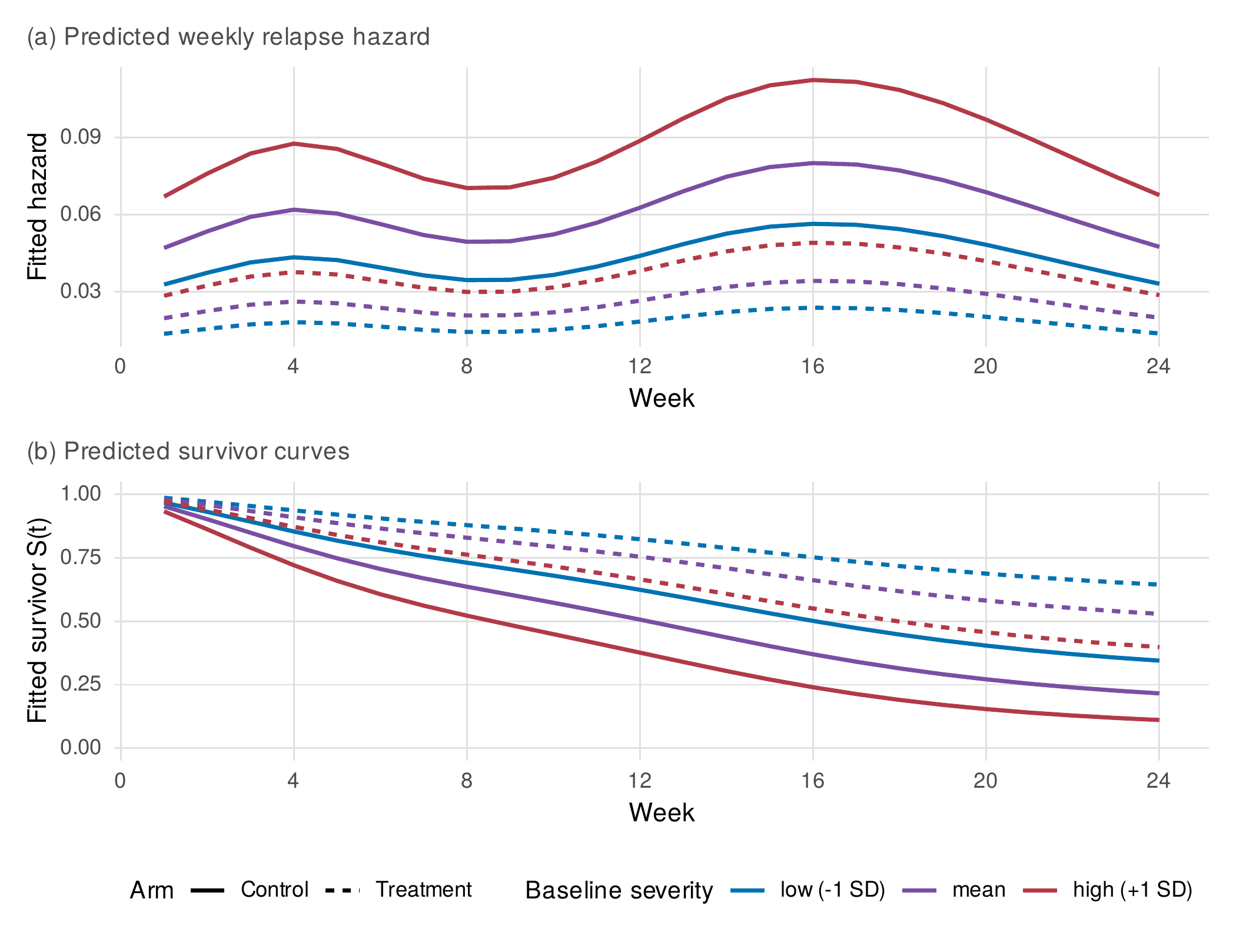
Note. Curves are from the natural-spline baseline logistic hazard model fitted to the relapse person-period file. Panel (a) gives the fitted weekly relapse hazard and panel (b) the implied survivor function \(S(t)=\prod_{k\le t}(1-h(k))\), for treatment and control arms (line type) crossed with baseline severity at minus one, zero, and plus one standard deviation (color). The humped baseline, the upward shift with severity, and the downward shift with treatment are all read directly from the fitted model.
The multilevel extension is the payoff of Chapter 15 arriving on schedule. Patients in the relapse study are nested in twenty-five treatment sites, and site-level differences in relapse risk, unmeasured therapist skill, local case mix, referral patterns, induce dependence among patients at the same site that a single-level model ignores. Adding a random intercept for site to the discrete-time hazard model, a one-line change from glm to glmer, recovers a site-level standard deviation of \(0.485\) on the logit scale, close to the value of \(0.50\) built into the generating process, and adjusts the covariate standard errors for the clustering. The random intercept is the discrete-time face of the shared-frailty models of Section 29.5; the two are the same idea, a latent multiplier on the hazard shared within a cluster, expressed once in logistic and once in Cox machinery.
29.3 Continuous Time: Kaplan-Meier and Cox
When time is measured finely enough that ties are rare, the continuous-time apparatus is more natural and more powerful. Its two instruments are the Kaplan-Meier estimator of the survivor function and the Cox model for the effect of covariates on the hazard. The Kaplan-Meier estimator (Kaplan & Meier, 1958) builds the survivor curve as a product over the distinct event times: at each time an event occurs, survival is multiplied by one minus the ratio of events to the risk set at that instant, and censored cases leave the risk set without triggering a drop. The result is the nonparametric survivor curve that uses every case for exactly its observed duration, and it is the honest picture that the naive means of Section 29.1 failed to produce. Figure 29.5 shows the Kaplan-Meier curves for the two treatment arms of the relapse data in the book’s house style, with the pointwise confidence bands and, beneath the plot, the number-at-risk table that every survival figure should carry. The median relapse-free time is eleven weeks in the control arm and twenty-two weeks in the treatment arm, and the separation between the curves is the treatment’s effect made visible.
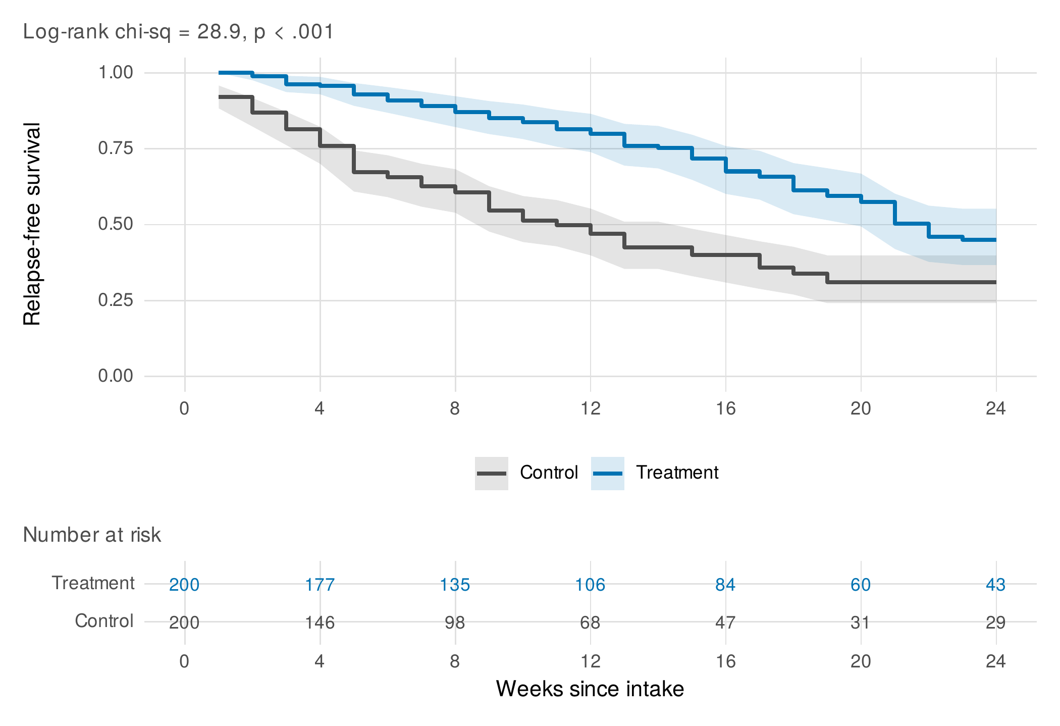
Note. Step functions are Kaplan-Meier estimates of the probability of remaining relapse-free; shaded bands are pointwise ninety-five percent confidence intervals. The number-at-risk table beneath the axis reports how many patients remain event-free and under observation at each four-week mark and is a required element of a survival figure, because the reliability of the right tail depends on how many patients are still at risk there. The log-rank test compares the whole curves.
The log-rank test compares two or more survivor curves by accumulating, at each event time, the difference between the observed number of events in a group and the number expected if the hazard were common across groups, then standardizing the sum. On the relapse arms it returns a chi-square of \(28.9\) on one degree of freedom, decisively rejecting equality of the curves. The test is most powerful when the hazards are proportional, a condition defined precisely below; when the curves cross, the accumulated differences partly cancel and the log-rank test loses power, a limitation that motivates its weighted relatives and, more importantly, motivates looking at the curves rather than trusting a single p-value.
The Cox proportional-hazards model (Cox, 1972) is the workhorse of continuous-time survival analysis, and its design is a piece of statistical elegance worth understanding rather than merely invoking. The model writes the hazard for a patient with covariates \(\mathbf{x}\) as \(h(t\mid\mathbf{x})=h_0(t)\exp(\mathbf{x}'\boldsymbol\beta)\), the product of an unspecified baseline hazard \(h_0(t)\) shared by everyone and a multiplier that depends on covariates but not on time. The baseline hazard is left completely unspecified, and yet the coefficients \(\boldsymbol\beta\) are estimated without it, through the partial likelihood. The idea is to condition on the set of event times and ask, at each event, which member of the current risk set was the one to have the event; under the model that probability is the individual’s hazard divided by the sum of hazards in the risk set, and the unknown baseline hazard, common to numerator and denominator, cancels. The product of these conditional probabilities over all events is the partial likelihood, and maximizing it estimates the hazard ratios while leaving the baseline shape as a nuisance to be recovered separately if wanted. On the relapse data the Cox model returns a treatment hazard ratio of \(0.415\) and a severity hazard ratio of \(1.44\) per standard deviation, agreeing with the discrete-time and complementary log-log fits, as they should.
Foundations Box • Why the baseline hazard drops out
At an event time \(t_{(j)}\), let \(R_j\) be the risk set, those still event-free and under observation just before \(t_{(j)}\). Under the Cox model the probability that the particular individual \(i_j\) who had the event was the one to have it, given that exactly one event occurred in \(R_j\), is \(\dfrac{h_0(t_{(j)})\exp(\mathbf{x}_{i_j}'\boldsymbol\beta)}{\sum_{\ell\in R_j} h_0(t_{(j)})\exp(\mathbf{x}_\ell'\boldsymbol\beta)}=\dfrac{\exp(\mathbf{x}_{i_j}'\boldsymbol\beta)}{\sum_{\ell\in R_j}\exp(\mathbf{x}_\ell'\boldsymbol\beta)}\). The baseline hazard \(h_0(t_{(j)})\) is common to every term and cancels, leaving a quantity that depends only on covariates and \(\boldsymbol\beta\). Multiplying these across all event times gives the partial likelihood. Tied event times, common in coarsely measured psychological data, break the clean derivation; the Efron approximation handles moderate ties well and is the sensible default, while heavy ties are a sign that a discrete-time model is the more honest choice.
The hazard ratio must be interpreted with a discipline that its convenience tends to erode. A hazard ratio is a ratio of instantaneous rates among those still at risk at each instant, and the risk set changes composition over time in ways the covariates do not fully capture. Even when a treatment has an identical effect on every patient, differential depletion of the risk set, the frailest patients relapsing first and leaving behind a hardier remainder, can make the hazard ratio drift toward one over follow-up, so that a constant hazard ratio is a strong assumption and a time-varying one is not evidence of a changing biological effect. Hernán (2010) presses this point to its conclusion: because the hazard ratio conditions on survival to each instant, and survival is affected by treatment, the hazard ratio at later times is a comparison of groups that are no longer exchangeable, and it does not have a clean causal interpretation as the effect of treatment on the timing of the event. The practical counsel is to read the hazard ratio as a useful summary of association, to report the survivor curves alongside it so the reader sees the absolute picture, and never to translate a hazard ratio into a statement about the probability of the event as though it were a risk ratio.
Common Pitfall • Three ways to misread a Cox model
The hazard ratio is not a risk ratio. A hazard ratio of \(0.4\) does not mean the treated group’s probability of the event is forty percent of the control group’s. It is a ratio of instantaneous rates conditional on survival; the effect on cumulative incidence depends on the baseline hazard and the follow-up length and must be read off the survivor or cumulative-incidence curves. The hazard ratio is not necessarily constant. A single reported hazard ratio assumes proportional hazards; if that assumption fails, the number is a time-average over a changing effect and can mislead badly, as the next figure shows. A hazard ratio at late follow-up is not a clean causal contrast. Conditioning on survival to time \(t\) conditions on a post-treatment variable, so late hazard ratios compare groups rendered non-exchangeable by the treatment itself (Hernán, 2010).
The proportional-hazards assumption is testable, and testing it is not optional. The Schoenfeld residuals, one per covariate per event, are the differences between a patient’s covariate value and the risk-set-weighted mean at the moment of the event; under proportional hazards they have no trend against time, and a trend is the signature of a covariate whose effect changes over follow-up (Grambsch & Therneau, 1994). The relapse data were built with a planted violation: the protective effect of treatment is strong early and fades over the six months, crossing to slightly harmful in the last weeks, a realistic pattern for a therapy whose benefit wanes without maintenance. The Schoenfeld test detects it decisively, with a chi-square of \(24.4\) on one degree of freedom for the treatment effect (the severity effect, built to be proportional, passes with a chi-square of \(0.76\)). Figure 29.6 shows the diagnostic and its remedy together. The scaled Schoenfeld residuals for treatment slope upward across time, and the constant-hazard-ratio line misses that slope; the resolution is to let the treatment coefficient vary with time, either as a step function across intervals or as a smooth function, and both recover the planted fade, the treatment log-hazard ratio rising from about \(-1.6\) in the first six weeks to about \(+1.0\) in the last six, crossing zero near week sixteen. Table 29.3 organizes the remedies.
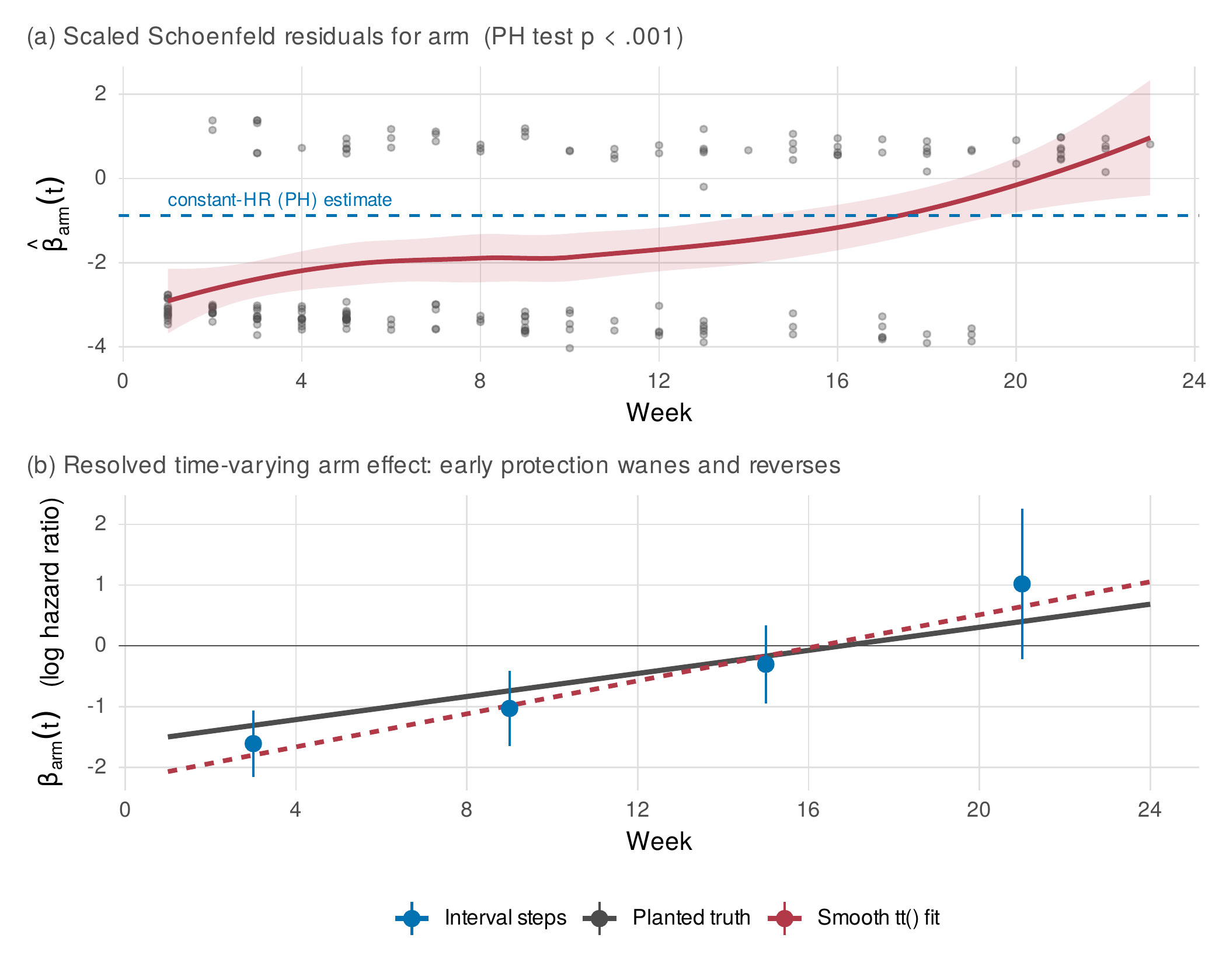
Note. Panel (a) plots the scaled Schoenfeld residuals for the treatment effect against time with a loess smooth; the upward trend, and the proportional-hazards test p-value below one in ten thousand, signal that the treatment effect is not constant. The dashed line is the single constant-hazard-ratio estimate, which the trend contradicts. Panel (b) resolves the violation: the interval-specific estimates (points with intervals) and the smooth time-varying fit (dashed) both track the planted truth (solid), a treatment effect that is strongly protective early and wanes to null and beyond. Reporting the single hazard ratio here would average a protective early effect with a harmful late one.
Table 29.3. A Ladder of Remedies for Proportional-Hazards Violations
| Remedy | What it does | When to prefer |
|---|---|---|
| Stratification | Lets the baseline hazard differ across strata; removes the offending variable from the hazard-ratio model | Nuisance variable; no interest in its effect |
| Time-varying coefficient | Estimates \(\beta(t)\) as a step or smooth function of time | The changing effect is of substantive interest |
| Interval-specific effects | Splits follow-up and reports a hazard ratio per interval | Communication; interpretable epochs |
| Accelerated failure time | Models time directly; different, often more stable, summary | When a time-scale effect is more natural |
| Report as is with caveat | Keep the average effect but state it is a time-average | Only when the violation is mild and disclosed |
Note. A proportional-hazards violation does not invalidate a study; it changes the estimand from a single hazard ratio to a time-varying one. The choice among remedies is driven by whether the offending variable is a nuisance to be absorbed or an effect to be described. Discarding the analysis is never the right response.
Functional form deserves the same scrutiny as proportionality. The martingale residuals from a Cox model that omits a continuous covariate, plotted against that covariate, reveal the shape in which the covariate should enter; a linear trend supports a linear term, and curvature calls for a spline, connecting to the additive-model machinery of Chapter 30. On the relapse data the martingale residuals against baseline severity are close to linear, supporting the linear severity term used throughout.
29.4 Time-Varying Covariates and Their Traps
Covariates need not be fixed at baseline. A patient’s symptom level, sleep quality, or medication adherence changes over follow-up, and a time-varying covariate lets the hazard at each instant depend on the covariate’s current value. The data structure that supports this is the counting-process format, in which each patient contributes a sequence of intervals \((t_{\text{start}},t_{\text{stop}}]\), each carrying the covariate values in force over that interval and an event indicator for its right endpoint. This is the same person-period logic as the discrete-time file, generalized to arbitrary interval boundaries. The intensive-measurement chapters of this book make time-varying covariates newly powerful: an ecological-momentary-assessment stream of daily symptom or craving reports can be aligned to the hazard of a clinical event, so that the question of whether momentary states forecast events, a distinctive contribution of intensive designs, becomes a survival model with a time-varying covariate. In the relapse data the weekly symptom score enters as a time-varying covariate, and the counting-process Cox model estimates its coefficient at \(0.29\) per point, so that a one-point-higher symptom score in a given week is associated with a thirty-four percent higher relapse hazard that week. This time-varying symptom outperforms the same patient’s baseline symptom score, whose coefficient is \(0.26\), because the current state carries information the baseline value has lost. Figure 29.7 shows the exhibit for six relapsing patients, their weekly symptom strips rising toward the relapse week.
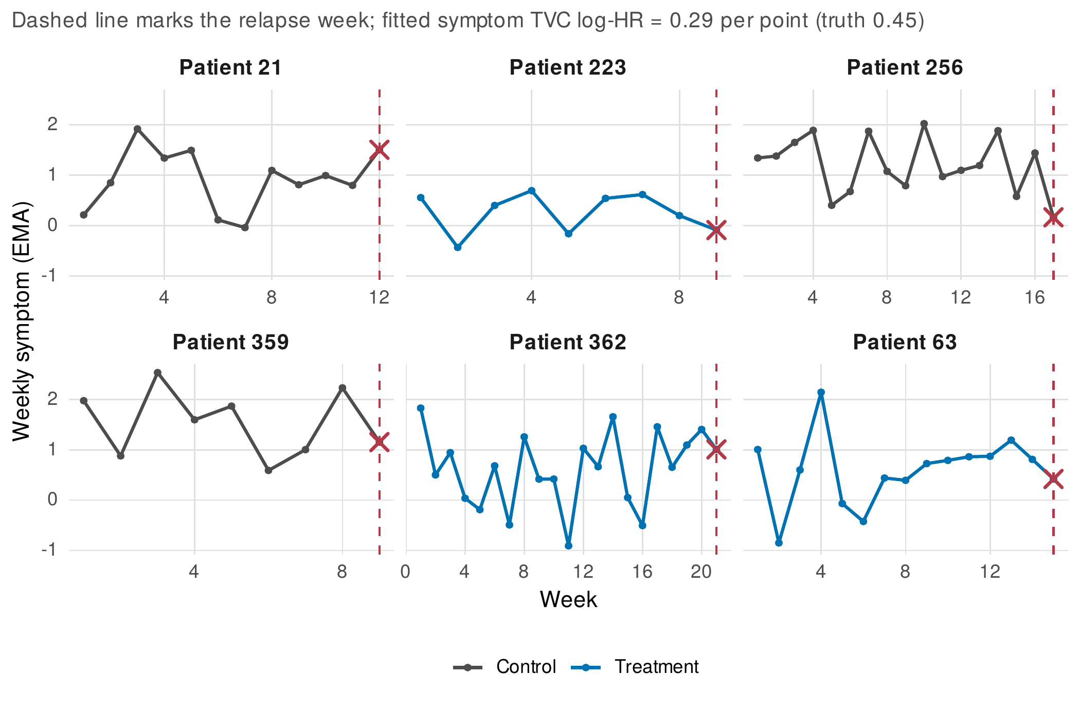
Note. Six patients who relapsed, with their weekly symptom (ecological-momentary-assessment) scores plotted to the relapse week (dashed line, cross). The current weekly symptom enters the hazard as a time-varying covariate; its fitted log-hazard ratio is \(0.29\) per point. The estimate is attenuated relative to the value of \(0.45\) built into the generating process because the observed weekly symptom is an error-prone reading of the latent state that actually drives the hazard, a regression-dilution effect that the joint model of Section 29.6 addresses. Patients shown are selected among relapsers with elevated late symptom to make the coupling visible.
Time-varying covariates split into two kinds whose difference is the hinge of the whole section. An exogenous (external) time-varying covariate follows a path that is not affected by the patient’s event status, such as season, age, or an externally set dose schedule; it can be entered into the Cox model directly and interpreted cleanly. An endogenous (internal) time-varying covariate is generated by the patient, is measured with error, and may itself respond to the impending event; the weekly symptom score is endogenous, because a patient sliding toward relapse has a rising symptom score for the same reason they are about to relapse. Entering an endogenous covariate in an ordinary Cox model is not wrong so much as limited: the coefficient is attenuated by measurement error, and the covariate’s own trajectory is left unmodeled, discarding information and mishandling the fact that the covariate stops being observed exactly when the patient has the event. The joint models of Section 29.6 are the correct home for endogenous covariates, and the appearance of the symptom score here is a deliberate setup for that payoff.
The most damaging trap in all of survival analysis lives in the mishandling of time-varying exposure, and it is worth a set piece. Immortal-time bias arises when a span of follow-up during which a patient could not, by construction, have had the event is misattributed to an exposure the patient had not yet received. The canonical illustration is the claim that Academy Award winners live longer than nominees who did not win, which foundered on exactly this error: an actor must survive to the award ceremony to win, so the years before winning are guaranteed event-free, and crediting them to the “winner” group manufactures a survival advantage from bookkeeping alone. When Sylvestre, Huszti, and Hanley (2006) reanalyzed the data treating award status as the time-varying covariate it is, giving each actor to the unexposed group until the moment of winning and to the exposed group thereafter, the advantage largely evaporated. The same structure recurs wherever exposure is defined by something that takes time to happen, responder analyses that classify patients by a response only survivors can exhibit, per-protocol analyses that require completing a course of treatment, analyses of transplantation that credit waiting time to the transplanted (Suissa, 2008). Figure 29.8 anatomizes the bias, and a focused simulation confirms it: with an exposure built to have exactly no effect, the naive analysis that classifies patients by ever-exposed and credits their pre-exposure time to the exposed group returns a spurious hazard ratio of \(0.28\), a large protective effect conjured from nothing, while the correct counting-process analysis that shifts each patient from unexposed to exposed at the true moment recovers a hazard ratio of \(1.03\), the null it should.
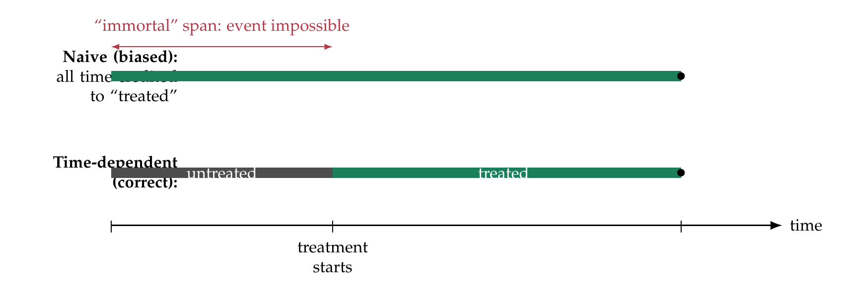
Note. A patient who begins treatment at time \(t_{rx}\) must survive event-free from intake to \(t_{rx}\) to be treated at all. The naive analysis (top) classifies the patient as treated for the entire follow-up, crediting the guaranteed-event-free “immortal” span before \(t_{rx}\) to the treated group and so manufacturing a survival advantage. The correct analysis (bottom) treats exposure as time-dependent, assigning the pre-treatment span to the untreated state and only the post-treatment span to the treated state. In a simulation with no true effect, the naive analysis returned a hazard ratio of \(0.28\) and the correct analysis \(1.03\).
29.5 Multilevel, Recurrent, and Competing Events
Three complications of real event data, clustering, repetition, and competition, each change the model in a way dictated by the substantive question. Shared frailty handles clustering by multiplying the hazard of every member of a cluster by a common latent factor, the frailty, drawn from a distribution with mean one and estimated variance; a gamma frailty is the conventional choice for its analytic convenience. On the relapse data, adding a gamma frailty for treatment site to the Cox model estimates a frailty variance of \(0.22\), close to the value implied by the generating process, and a likelihood-ratio test against the no-frailty model is decisive, confirming that sites differ in relapse risk beyond what the covariates explain. The frailty variance is interpretable as the amount of unexplained between-cluster heterogeneity in the hazard, and it is the continuous-time twin of the site random intercept from the discrete-time model of Section 29.2; the treatment effect is essentially unchanged by the frailty, as it should be when treatment is balanced across sites, but its standard error is honestly enlarged.
Repetition asks a prior question, what counts as the event. When events can recur, lapses in a cessation attempt, aggressive incidents, hospital readmissions, the analyst must decide whether the quantity of interest is the overall rate of events or the risk of the next event given the number already experienced, and the two questions call for different models. Table 29.4 lays out the choices. The Andersen-Gill model (Andersen & Gill, 1982) treats each patient as a counting process with a common baseline hazard and intervals between successive events all contributing to a single risk set; it estimates an overall rate ratio and answers the population-rate question, with robust standard errors to accommodate the within-patient dependence. The Prentice-Williams-Peterson model (Prentice et al., 1981) stratifies by event number, so that the risk of a first event, a second event, and a third are governed by separate baseline hazards, and it answers the conditional, episode-specific question. Figure 29.9 contrasts their risk-set constructions. A focused simulation of recurrent lapses with a covariate built to halve the lapse rate recovers the truth under both models, the Andersen-Gill log-rate-ratio at \(-0.47\) and the Prentice-Williams-Peterson at \(-0.45\) against a planted \(-0.50\), but the two estimands would diverge if the covariate’s effect differed across episodes, and the choice between them should be made by the question, not by which fits better.
Table 29.4. Choosing a Recurrent-Event Model by the Question
| Model | Estimand | Use when |
|---|---|---|
| Andersen-Gill | Overall event rate ratio | The total burden or rate of events is the outcome; effects assumed common across episodes |
| Prentice-Williams-Peterson | Episode-specific hazard ratios (stratified by event number) | Risk of the next event given history; effects may differ by episode |
| Frailty (random effect) | Rate ratio with explicit within-person heterogeneity | Between-person variation in proneness is of interest |
Note. All three use the counting-process data layout. Andersen-Gill and frailty target a rate; Prentice-Williams-Peterson targets episode-conditional risk. Robust or model-based standard errors accommodate the dependence among a person’s repeated events. The models answer different questions and can give different answers; the question comes first.
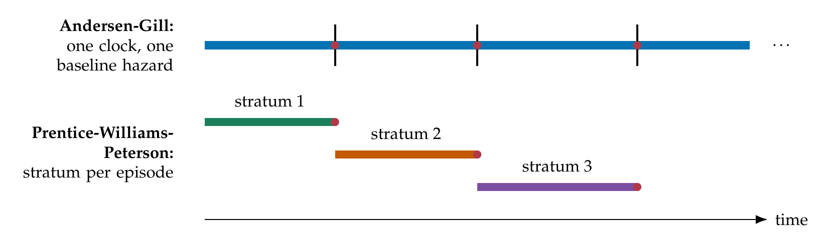
Note. Red dots are a single patient’s successive events. The Andersen-Gill model (top) places all inter-event intervals on one clock under a common baseline hazard and estimates an overall rate ratio. The Prentice-Williams-Peterson model (bottom) assigns each successive episode to its own stratum with its own baseline hazard, so the risk of a second event is modeled separately from the risk of a first, answering an episode-conditional question. The layouts encode different estimands, not different fits of the same estimand.
Competition is the subtlest of the three, because it silently invalidates the tool most analysts reach for first. Competing risks arise when more than one type of event can end follow-up and the occurrence of one removes the possibility of another: in the relapse data a patient who drops out of care can no longer be observed to relapse, so dropout competes with relapse. The error to avoid is estimating the cumulative incidence of relapse by one minus the Kaplan-Meier curve while treating dropout as ordinary censoring, because that treats the dropped patients as though they remained at risk of the relapse we would have seen, inflating the estimated relapse incidence. The correct object is the cumulative incidence function, which counts only the relapses actually reached and accounts for the depletion of the risk set by the competing event. Figure 29.10 shows the gap: the one-minus-Kaplan-Meier curve lies well above the cumulative incidence function in both arms, and the discrepancy grows as dropout accumulates, so a study that reported the former would overstate the burden of relapse.
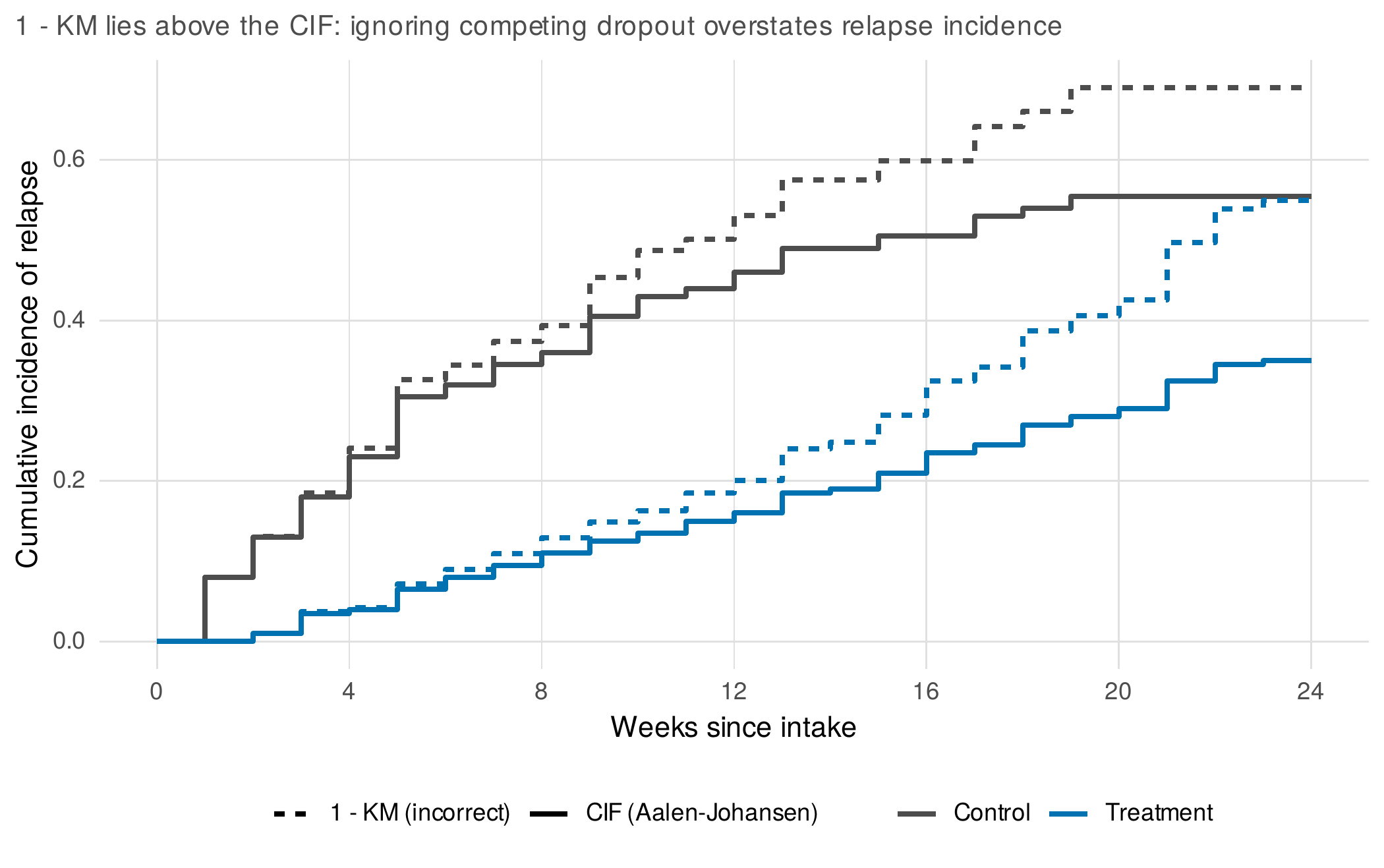
Note. For each treatment arm, the solid curve is the cumulative incidence function for relapse, which accounts for the competing risk of dropout, and the dashed curve is one minus the Kaplan-Meier estimate, which treats dropout as though it were noninformative censoring of relapse. The dashed curve lies above the solid one because it credits the dropped patients with relapses they were never observed to have; the gap widens with follow-up as dropout accumulates. Reporting one minus Kaplan-Meier under competing risks overstates the incidence of the event of interest.
Two estimands live under the competing-risks heading, and they answer different scientific questions. The cause-specific hazard is the instantaneous rate of relapse among those still relapse-free and still in care; it is estimated by a Cox model that censors the competing dropout, and it answers the etiologic question of how a covariate influences the biological process leading to relapse. The subdistribution hazard of Fine and Gray (1999) keeps patients who had the competing event in the risk set with a declining weight, so that its coefficient maps directly onto the cumulative incidence function; it answers the prognostic question of how a covariate influences the actual probability of relapse in a population where dropout also occurs. On the relapse data the cause-specific treatment log-hazard is \(-0.88\) and the Fine-Gray subdistribution log-hazard is \(-0.81\), close here because treatment does not much affect dropout, but they are different estimands and can diverge sharply when a covariate affects the competing event, as Table 29.5 sets out. The rule is to name the question first: for mechanism, cause-specific; for prediction and for the cumulative incidence a clinician needs, Fine-Gray (Austin et al., 2016).
Table 29.5. Cause-Specific Versus Subdistribution Hazards
| Feature | Cause-specific hazard | Subdistribution (Fine-Gray) |
|---|---|---|
| Risk set | Removes competing-event cases at their event time (censors them) | Keeps competing-event cases with decreasing weight |
| Maps to | The rate of the event among the still-at-risk | The cumulative incidence function |
| Answers | Etiology: effect on the process generating the event | Incidence/prognosis: effect on the actual probability |
relapse arm effect | \(-0.88\) (log-hazard) | \(-0.81\) (log-subdistribution-hazard) |
| Report when | Studying mechanism; both causes modeled together | Predicting absolute risk; clinical incidence |
Note. The two hazards coincide only when the covariate has no effect on the competing event. Because they answer different questions, a complete competing-risks analysis often reports both: the cause-specific hazards for each cause to describe the mechanisms, and the cumulative incidence functions (with Fine-Gray effects) to describe the resulting absolute risks.
In Practice • Rare events and the events-per-variable heuristic
Psychological event studies are often small and their events rare, and the binding constraint is not the sample size but the number of events. A widely used rule of thumb asks for at least ten to fifteen events per estimated coefficient in a Cox or discrete-time model; below that, coefficients are unstable and their standard errors optimistic. With a seven-percent event rate in a sample of three hundred, only about twenty-one events are available, enough for one or two covariates, not five. The honest responses are to reduce the number of covariates by prespecification, to use penalized (ridge or lasso) partial likelihood to stabilize estimation, to coarsen to a discrete-time model that pools information across periods, or to report the analysis as exploratory. Reporting a ten-covariate Cox model on twenty events as though its p-values meant what they say is the failure this heuristic exists to prevent.
29.6 Joint Longitudinal-Survival Models
The chapter’s final model closes two loops at once. The endogenous time-varying covariate of Section 29.4 was left improperly handled, entered into the hazard with its measurement error intact and its own trajectory unmodeled. The outcome-dependent dropout of Chapter 6, promised there a shared-parameter treatment, was left as an assumption. The joint longitudinal-survival model resolves both by fitting two submodels simultaneously and linking them through shared random effects. The longitudinal submodel is the growth model of Chapters 13 and 14, a mixed model for the repeated measurements with random intercepts and slopes. The survival submodel is a hazard model for the event, here the informative dropout, whose linear predictor includes a function of the same random effects that generate the trajectory. Because the two submodels share the random effects, the association between a patient’s symptom trajectory and their risk of dropping out is estimated rather than ignored, and the longitudinal parameters are corrected for the selection that dropout imposes. Figure 29.11 draws the architecture and shows the payoff.
The association can be parameterized in several ways, and the choice encodes a hypothesis about how the trajectory drives the event. Table 29.6 lays them out. The current-value parameterization links the hazard to the trajectory’s fitted level at each instant, appropriate when it is the present state that matters, a symptom level crossing a threshold. The slope parameterization links the hazard to the rate of change, appropriate when it is deterioration or improvement that drives the event regardless of level. The shared-random-effects parameterization links the hazard directly to the random effects, the parsimonious choice that ties the event to a patient’s stable individual tendencies. The relapse generating process was built with dropout depending on a patient’s random slope, so patients deteriorating fastest leave earliest, the paradigm case of missing-not-at-random attrition, and the shared-random-effects parameterization is the matching model. Because the competing terminal event of relapse makes the full relapse data a harder case than a single two-part model specifies, the payoff is demonstrated on a focused simulation isolating the dropout mechanism, in the same spirit as the immortal-time and recurrent-event set pieces.
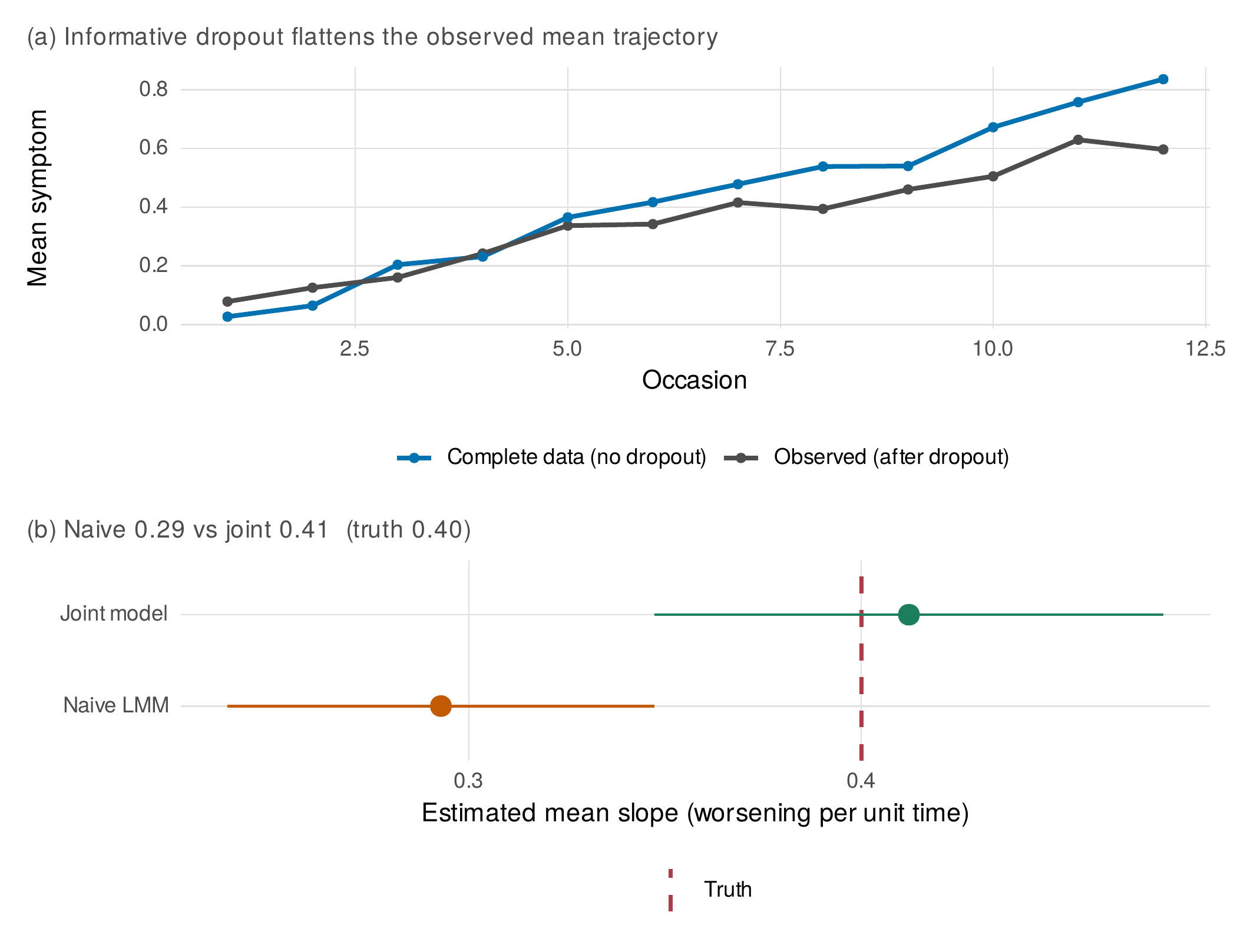
Note. Top: the longitudinal (growth) submodel and the survival (dropout) submodel share the patient random effects, so the association between trajectory and dropout is modeled rather than assumed absent. Bottom panel (a): because patients who deteriorate fastest drop out earliest, the observed mean trajectory (after dropout) flattens relative to the complete-data mean, the signature of missing-not-at-random attrition. Bottom panel (b): the naive mixed model, fitted to the observed data alone, estimates the mean worsening slope at \(0.29\), biased below the true \(0.40\); the shared-parameter joint model recovers \(0.41\), and the association parameter is estimated at its true value. The naive analysis understates deterioration precisely because the deteriorating patients are the ones who leave.
The payoff is the exhibit that justifies the machinery. In the focused simulation the population mean worsening slope is \(0.40\) by construction, and a complete-data mixed model recovers it at \(0.395\). But dropout removes the fastest deteriorators, so the observed trajectories are a selected sample, and the naive mixed model fitted to the observed data alone estimates the slope at \(0.29\), understating the deterioration by more than a quarter, because the patients whose worsening would have pulled the mean upward have left. The shared-parameter joint model, fitting the dropout hazard and the trajectory together with the random slope shared between them, recovers the slope at \(0.41\) and estimates the association parameter at its true value. This is the concrete meaning of the shared-parameter approach to missing-not-at-random data promised in Chapter 6: the dropout is not assumed ignorable, it is modeled, and the modeling repairs the bias that ignoring it would have caused. The correction is only as good as the assumed association structure, which is untestable from the observed data in the same way the missing-at-random assumption is, so a joint-model analysis is properly reported as a principled sensitivity analysis, an answer to the question of what the trajectory looks like if dropout depends on the random effects in the specified way, set beside the naive answer that assumes it does not.
Table 29.6. Association Parameterizations in Joint Models
| Parameterization | Hazard depends on | Substantive reading |
|---|---|---|
| Current value | Fitted trajectory level \(m_i(t)\) at time \(t\) | The present state drives the event (threshold crossing) |
| Slope | Rate of change \(m_i'(t)\) | Deterioration or improvement drives the event regardless of level |
| Shared random effects | The random effects \(b_i\) directly | Stable individual tendencies drive the event |
| Current value + slope | Both level and rate | Level and its direction both matter |
Note. The parameterization is a scientific hypothesis about how the trajectory couples to the event, not a technical detail. It should be chosen a priori from theory and, where competing forms are plausible, compared by information criteria. The relapse generating process couples dropout to the random slope, so the shared-random-effects form is the matching specification.
Software Note • Fitting joint models in R
Fitting joint models well requires dedicated software, because the likelihood integrates over the random effects for both submodels at once. In R the mature choices are the JM package and its Bayesian successor JMbayes2, which fit a wide range of association structures, competing and recurrent events, and multivariate longitudinal markers; joineRML handles multiple longitudinal outcomes by maximum likelihood. Package capabilities and defaults change, so the current documentation should be consulted rather than a remembered interface. The worked example in this chapter uses a hand-written maximum-likelihood fit with Gauss-Hermite integration over the two random effects, adequate for a single longitudinal marker and a single event and transparent as to what the likelihood contains, but production analyses with several markers or event types belong in the dedicated packages, whose numerical machinery is built for the scale.
29.7 Reporting a Survival Analysis
A survival analysis is reported to a standard that makes its handling of censoring and its choice of estimand explicit, because those are the decisions on which its validity turns and the ones a reader cannot reconstruct from a hazard ratio alone. Table 29.7 is the checklist. The origin of time and the definition of the event must be stated precisely, because a hazard is meaningless without them. The censoring must be described, its extent quantified, and its plausible informativeness discussed rather than waved past, with the competing events named and handled by an estimand that matches the question. The proportional-hazards assumption, if a Cox model is used, must be checked and the check reported, with the remedy named if the assumption fails. The figures carry the argument: a Kaplan-Meier or cumulative-incidence display with a number-at-risk table, and a predicted-curve display for the covariate effects of interest, communicate what a table of hazard ratios cannot.
Table 29.7. Reporting Checklist for Survival Analyses
| Element | What to report |
|---|---|
| Time origin and event | The precise start of the clock and the event definition; the time metric (continuous or discrete) |
| Censoring | Extent (percent censored), types present, and an argument for or against noninformativeness |
| Risk sets | Sample size, number of events, and events per variable; number-at-risk tables on curves |
| Model and estimand | Discrete-time, Cox, or parametric; hazard ratios with intervals; the estimand named |
| Proportional hazards | The diagnostic performed and its result; the remedy if violated |
| Competing risks | Named competing events; cause-specific and/or Fine-Gray, matched to the question |
| Figures | Survivor or cumulative-incidence curves with risk tables; predicted-curve displays |
Note. The reporting standard for survival analysis is organized around the two decisions a reader cannot otherwise verify: how censoring was handled and which estimand the reported effects target. Stating the time origin, quantifying censoring, checking proportional hazards, and naming the competing-risks estimand are the elements most often missing and most consequential when absent.
A results paragraph for the relapse analysis, written to this standard, reads as follows. Of four hundred patients followed for up to twenty-four weeks from intake, one hundred eighty-one (forty-five percent) relapsed, one hundred forty-eight (thirty-seven percent) left care before relapse (a competing event), and seventy-one (eighteen percent) remained in remission at the administrative end; median relapse-free time was eleven weeks in the control arm and twenty-two weeks in the treatment arm. A Cox model estimated a treatment hazard ratio of \(0.42\), but the proportional-hazards assumption was violated for treatment (Schoenfeld test, \(p<.001\)), so the effect was modeled as time-varying: treatment was strongly protective in the first weeks (log-hazard ratio near \(-1.6\)) and its benefit waned to null by the study’s end, indicating that the protection was not maintained. Baseline severity raised the relapse hazard (hazard ratio \(1.44\) per standard deviation) with a proportional effect. Accounting for the competing risk of dropout, the cumulative incidence of relapse at twenty-four weeks was substantially lower than a one-minus-Kaplan-Meier estimate would suggest, and a joint longitudinal-survival model indicated that dropout was associated with faster symptom deterioration, so that a growth model ignoring dropout understated the average worsening. This paragraph states the origin, quantifies the censoring and the competing event, names the proportional-hazards violation and its resolution, distinguishes the estimands, and reports the missing-not-at-random sensitivity, which is the whole of the discipline this chapter teaches.
Chapter Summary
Timing-of-event questions require their own machinery because censoring, the known-only-to-exceed status of participants without the event at the study’s end, biases every naive summary: on the relapse data the mean of observed relapse times, the mean treating censoring as the event, and an ordinary regression on follow-up time all miss the Kaplan-Meier median badly. The hazard is the central quantity because it is defined among those still at risk and so absorbs censoring, and the survivor function is recovered from it by accumulating survival. Discrete-time survival is the psychologist’s entry: the person-period file turns event data into a logistic regression, the baseline hazard is specified by dummies, polynomials, or splines, covariate effects read as hazard-odds ratios, and the complementary log-log link recovers the continuous-time hazard ratio; a site random intercept adds multilevel structure with Chapter 15’s tools. In continuous time the Kaplan-Meier estimator and the log-rank test summarize and compare survivor curves, and the Cox model estimates hazard ratios through a partial likelihood in which the unspecified baseline hazard cancels. The hazard ratio must be read as a conditional, among-survivors rate ratio, never as a risk ratio, and its constancy checked with Schoenfeld residuals; the relapse data carry a planted proportional-hazards violation that the residuals detect and a time-varying coefficient resolves, recovering a treatment benefit that wanes over follow-up. Time-varying covariates enter through counting-process data and let intensive-measurement streams forecast events, but endogenous covariates are attenuated and belong in joint models, and immortal-time bias, the misattribution of guaranteed-event-free time to an exposure not yet received, manufactures effects from nothing, as a null simulation returning a spurious hazard ratio of \(0.28\) demonstrates. Clustering is handled by shared frailty, repetition by Andersen-Gill or Prentice-Williams-Peterson models chosen by whether the rate or the episode-specific risk is the question, and competition by cumulative incidence functions rather than one minus Kaplan-Meier, with cause-specific and Fine-Gray hazards answering the etiologic and the prognostic questions respectively. The joint longitudinal-survival model links a growth submodel and a hazard submodel through shared random effects, delivering the shared-parameter treatment of missing-not-at-random dropout promised in Chapter 6: when dropout depends on the symptom slope, a naive growth model understates deterioration and the joint model recovers it. Reporting is organized around the two decisions a reader cannot otherwise verify, how censoring was handled and which estimand the effects target.
Allison, P. D. (1982). Discrete-time methods for the analysis of event histories. Sociological Methodology, 13, 61–98. https://doi.org/10.2307/270718
Andersen, P. K., & Gill, R. D. (1982). Cox’s regression model for counting processes: A large sample study. The Annals of Statistics, 10(4), 1100–1120. https://doi.org/10.1214/aos/1176345976
Austin, P. C., Lee, D. S., & Fine, J. P. (2016). Introduction to the analysis of survival data in the presence of competing risks. Circulation, 133(6), 601–609. https://doi.org/10.1161/CIRCULATIONAHA.115.017719
Cox, D. R. (1972). Regression models and life-tables. Journal of the Royal Statistical Society: Series B (Methodological), 34(2), 187–202. https://doi.org/10.1111/j.2517-6161.1972.tb00899.x
Fine, J. P., & Gray, R. J. (1999). A proportional hazards model for the subdistribution of a competing risk. Journal of the American Statistical Association, 94(446), 496–509. https://doi.org/10.1080/01621459.1999.10474144
Grambsch, P. M., & Therneau, T. M. (1994). Proportional hazards tests and diagnostics based on weighted residuals. Biometrika, 81(3), 515–526. https://doi.org/10.1093/biomet/81.3.515
Henderson, R., Diggle, P., & Dobson, A. (2000). Joint modelling of longitudinal measurements and event time data. Biostatistics, 1(4), 465–480. https://doi.org/10.1093/biostatistics/1.4.465
Hernán, M. A. (2010). The hazards of hazard ratios. Epidemiology, 21(1), 13–15. https://doi.org/10.1097/EDE.0b013e3181c1ea43
Hougaard, P. (2000). Analysis of multivariate survival data. Springer. https://doi.org/10.1007/978-1-4612-1304-8
Kaplan, E. L., & Meier, P. (1958). Nonparametric estimation from incomplete observations. Journal of the American Statistical Association, 53(282), 457–481. https://doi.org/10.1080/01621459.1958.10501452
Muthén, B., & Masyn, K. (2005). Discrete-time survival mixture analysis. Journal of Educational and Behavioral Statistics, 30(1), 27–58. https://doi.org/10.3102/10769986030001027
Prentice, R. L., Williams, B. J., & Peterson, A. V. (1981). On the regression analysis of multivariate failure time data. Biometrika, 68(2), 373–379. https://doi.org/10.1093/biomet/68.2.373
Rizopoulos, D. (2010). JM: An R package for the joint modelling of longitudinal and time-to-event data. Journal of Statistical Software, 35(9), 1–33. https://doi.org/10.18637/jss.v035.i09
Rizopoulos, D. (2012). Joint models for longitudinal and time-to-event data: With applications in R. Chapman & Hall/CRC.
Singer, J. D., & Willett, J. B. (1991). Modeling the days of our lives: Using survival analysis when designing and analyzing longitudinal studies of duration and the timing of events. Psychological Bulletin, 110(2), 268–290. https://doi.org/10.1037/0033-2909.110.2.268
Singer, J. D., & Willett, J. B. (1993). It’s about time: Using discrete-time survival analysis to study duration and the timing of events. Journal of Educational Statistics, 18(2), 155–195. https://doi.org/10.3102/10769986018002155
Singer, J. D., & Willett, J. B. (2003). Applied longitudinal data analysis: Modeling change and event occurrence. Oxford University Press.
Stoolmiller, M., & Snyder, J. (2006). Modeling heterogeneity in social interaction processes using multilevel survival analysis. Psychological Methods, 11(2), 164–177. https://doi.org/10.1037/1082-989X.11.2.164
Suissa, S. (2008). Immortal time bias in pharmacoepidemiology. American Journal of Epidemiology, 167(4), 492–499. https://doi.org/10.1093/aje/kwm324
Sylvestre, M.-P., Huszti, E., & Hanley, J. A. (2006). Do Oscar winners live longer than less successful peers? A reanalysis of the evidence. Annals of Internal Medicine, 145(5), 361–363. https://doi.org/10.7326/0003-4819-145-5-200609050-00009
Therneau, T. M., & Grambsch, P. M. (2000). Modeling survival data: Extending the Cox model. Springer. https://doi.org/10.1007/978-1-4757-3294-8
Willett, J. B., & Singer, J. D. (1995). It’s déjà vu all over again: Using multiple-spell discrete-time survival analysis. Journal of Educational and Behavioral Statistics, 20(1), 41–67. https://doi.org/10.3102/10769986020001041