Chapter 30
Flexible Curves: GAMMs, TVEM, and Functional Data Approaches
The growth models of Chapters 13 and 14 asked the analyst to commit, before seeing the data, to the algebraic form of change: linear, quadratic, piecewise, exponential. When the commitment is right, parametric growth is efficient and interpretable. When it is wrong, the misfit is not random but systematic, and a polynomial forced onto a curve it does not match will invent features in the tails that are artifacts of the basis rather than facts about development. This chapter develops the machinery that lets the data speak about shape while keeping inference honest. Penalized splines represent a curve in a basis rich enough to bend wherever the data require and then discipline that freedom with a wiggliness penalty whose strength is chosen by the data rather than the analyst’s eye, so that the fitted curve carries a genuine confidence band rather than the false precision of a parametric form assumed correct. Generalized additive mixed models graft this flexibility onto the random-effects structure of the whole book, and the connection runs deep: a smooth is a random effect, and the smoothing parameter is a variance ratio, so flexibility is continuous with the mixed-model thinking already in hand rather than a departure from it. The chapter then turns the flexibility onto the coefficients themselves. Time-varying effect models ask not what shape an outcome traces but what shape a predictor’s effect traces: whether a treatment’s benefit emerges and wanes, whether a stressor’s grip habituates across a study. It closes with a working introduction to functional data analysis, in which an entire curve is the unit of analysis, registration separates the timing of an event from its magnitude, and functional principal components play the role that growth factors played in Chapter 19. Throughout, the discipline matters as much as the machinery: a smooth that finds a dip is a hypothesis about a dip, not a discovery of one, and the chapter teaches the diagnostics and the reporting that keep flexible models from narrating noise.
Learning Objectives
After working through this chapter, you should be able to: (1) explain penalized splines as a rich basis plus a wiggliness penalty, read the effective degrees of freedom as the amount of shape the data earned, and describe how restricted maximum likelihood chooses the smoothing parameter; (2) fit generalized additive mixed models that combine population smooths with random intercepts, random slopes, and nonparametric person-specific smooths, and know the two routes mgcv offers; (3) perform inference on smooths with pointwise and simultaneous bands and compare groups with a difference smooth; (4) model cyclic phenomena with cyclic splines and weigh them against the trigonometric approach of Chapter 23; (5) specify time-varying effect models in which a coefficient is a smooth function of time, and say what question they answer that a parametric interaction does not; (6) understand functional data analysis at working depth, including registration, functional principal components as the analogue of growth factors, and when the machinery earns its cost; and (7) recognize and prevent the abuses of flexible models, from concurvity to the narration of wiggles a band does not support.
30.1 Why Flexibility, Disciplined
The case for flexible curve estimation begins with a failure of the parametric alternative. When a developmental process is genuinely nonlinear in a way no low-order polynomial captures, fitting a polynomial does not merely lose a little efficiency; it produces a fitted curve whose shape is dictated by the basis rather than the phenomenon, bending upward at the ends to accommodate a middle it cannot otherwise reach, and reporting these basis artifacts with the same confidence intervals it attaches to real structure. The alternative of pre-binning time into named phases, an early phase and a late phase with a mean in each, is worse, because it imposes a step function on a continuous process and hides the imposition inside the phase definitions. The growth_gam data, a simulated study of two hundred fifty children measured at irregular ages between six and fifteen and nested in twenty schools, are generated from a logistic growth spurt: achievement is nearly flat in the early years, rises steeply around age ten, and levels off, a shape with flat tails and a steep middle that a quadratic cannot represent. Fitted to these data, a quadratic misses by a root-mean-squared error of \(0.95\) against the known truth and a broken-stick model by \(0.99\), while the penalized smooth developed below misses by \(0.17\). The lesson is not that polynomials are never right but that their rightness is an assumption to be earned, and that a method which lets the data choose the shape, and reports honest uncertainty about that choice, is the safer default when theory does not pin the form.
The penalized spline is that method, and its anatomy is worth seeing before its machinery is used. A smooth function is written as a weighted sum of a fixed set of basis functions, small localized bumps spread across the range of the predictor, so that any sufficiently rich basis can approximate any smooth shape by an appropriate choice of weights. Fitting the weights by ordinary least squares with a rich basis would interpolate the noise, so the fit adds a penalty on wiggliness, typically the integrated squared second derivative of the curve, which measures how much the curve bends. The estimate minimizes the sum of the lack of fit and the penalty times a smoothing parameter, and that smoothing parameter is the single dial that trades bias against variance: at zero it returns the wiggly interpolant, at infinity it returns the straight line the penalty cannot touch, and in between it returns a curve as flexible as the data support. Figure 30.1 shows the basis and the three regimes on a simulated function. The crucial move, the one that separates penalized regression from exploratory curve-drawing, is that the smoothing parameter is estimated from the data by restricted maximum likelihood, not set by the analyst’s judgment of how smooth the curve should look. The effective degrees of freedom, the trace of the smoother matrix, summarizes how much shape the data bought: a curve that turns out linear spends one degree of freedom, a gently curved one spends three or four, and the simulated function in the figure earns about seven at the restricted-maximum-likelihood optimum, against nineteen available in the basis.
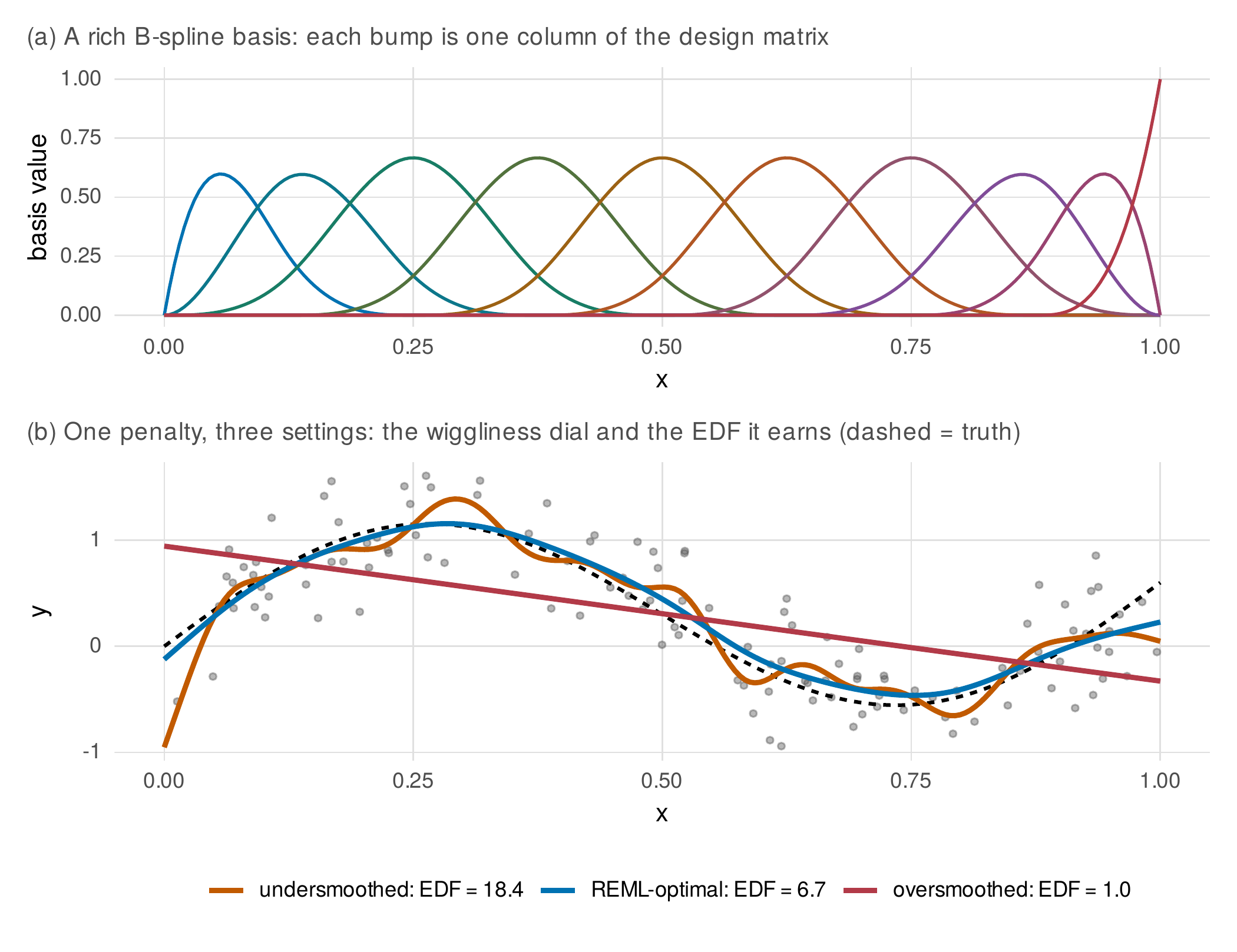
Note. Panel (a) shows a rich B-spline basis; a smooth is a weighted sum of these bumps. Panel (b) shows the penalized fit to a simulated function (dashed) at three settings of the smoothing parameter. Oversmoothing (one effective degree of freedom) returns a straight line that misses the shape; undersmoothing (eighteen effective degrees of freedom) chases the noise; the restricted-maximum-likelihood choice (about seven) recovers the truth. The smoothing parameter is the bias-variance dial, and it is chosen by the data, not the eye.
The depth of the idea is that the penalty is a prior and the smooth is a random effect. Splitting the basis into an unpenalized part, the functions the penalty leaves alone, and a penalized part, the penalty shrinks the penalized coefficients toward zero exactly as a mixed model shrinks random effects toward their mean, and the smoothing parameter turns out to be the ratio of the residual variance to the variance of those random coefficients. This is not an analogy but an identity: a penalized spline is a linear mixed model in which the wiggly part of the curve is a random effect, and the restricted-maximum-likelihood machinery of Chapter 13 selects the smoothing parameter as it selects any variance component. The identity is what makes generalized additive mixed models coherent, because once a smooth is a random effect it lives naturally alongside the random intercepts and slopes of the longitudinal models the book has been building, and the whole apparatus is estimated together. Table 30.1 organizes the basis types the rest of the chapter uses, and the foundations box states the mixed-model representation precisely.
Table 30.1. A Selector for Spline Basis Types in mgcv
Basis (bs=) | Name | Use for |
|---|---|---|
"tp" / "cr" | Thin-plate / cubic | The default smooth of a continuous predictor (age, time) |
"cc" | Cyclic cubic | A predictor that wraps: time of day, day of year, phase |
"fs" | Factor-smooth | A separate smooth per person or group sharing one penalty: nonparametric random trajectories |
"re" | Random effect | Random intercepts or slopes written as a smooth (the mixed-model route) |
by= | By-variable | A smooth that multiplies a covariate (varying coefficient) or differs by a factor (difference smooth) |
Note. The by= argument is the workhorse of Sections 30.2 and 30.3: with a factor it produces a separate or difference smooth per group, and with a numeric covariate it produces a varying coefficient, a smooth that scales the covariate’s effect across time. The factor-smooth ("fs") and random-effect ("re") bases are how random effects enter a generalized additive mixed model.
Foundations Box • A smooth is a random effect
Write a penalized smooth as \(f(x)=X\boldsymbol\beta\) with wiggliness penalty \(\lambda\,\boldsymbol\beta'S\boldsymbol\beta\). Reparameterize so the penalty is diagonal and separate the null space of \(S\) (functions with zero penalty, typically the constant and linear terms) from its range (the penalized, wiggly functions). The penalized coefficients enter the fit exactly as random effects with covariance \(\sigma^2/\lambda\) times the identity, so the penalized log-likelihood equals the log-likelihood of a linear mixed model in which the wiggly part of the curve is random. The smoothing parameter is a variance ratio, \(\lambda=\sigma^2_\varepsilon/\sigma^2_b\): a small random-coefficient variance means a stiff curve, a large one a flexible curve. Restricted maximum likelihood therefore selects the smoothing parameter as the variance-component estimation of Chapter 13, which is why generalized additive mixed models and linear mixed models are one framework, and why the shrinkage intuition of random effects transfers directly to the shrinkage of a curve toward smoothness.
30.2 Generalized Additive Mixed Models for Longitudinal Data
A generalized additive mixed model adds smooths of predictors to the random-effects structure of a mixed model, and mgcv offers two routes to it. The function gamm fits the model through its linear-mixed-model representation using nlme, which makes correlated residuals available, while gam with a random-effect basis (bs="re") or a factor-smooth basis (bs="fs") fits the same class through penalized likelihood, which is faster and, in the bam variant, scales to the large data sets that intensive longitudinal designs produce. For the growth_gam data the model of first resort is a population smooth of age plus a school random intercept, and it recovers the logistic truth with an effective degrees of freedom of \(7.4\) for the age smooth and a school standard deviation of \(1.04\) against a true value of \(1.2\). The diagnostic that guards this fit is the basis-dimension check: the basis size \(k\) is a ceiling on flexibility, not a choice of it, and mgcv’s gam.check reports whether the ceiling binds by testing the residuals for leftover pattern at the scale of the smooth. Here the check returns a \(k\)-index of \(1.02\) with a nonsignificant p-value, indicating the basis is large enough that the penalty, not the ceiling, is doing the smoothing. Figure 30.2 contrasts the smooth with the parametric alternatives against the known truth.
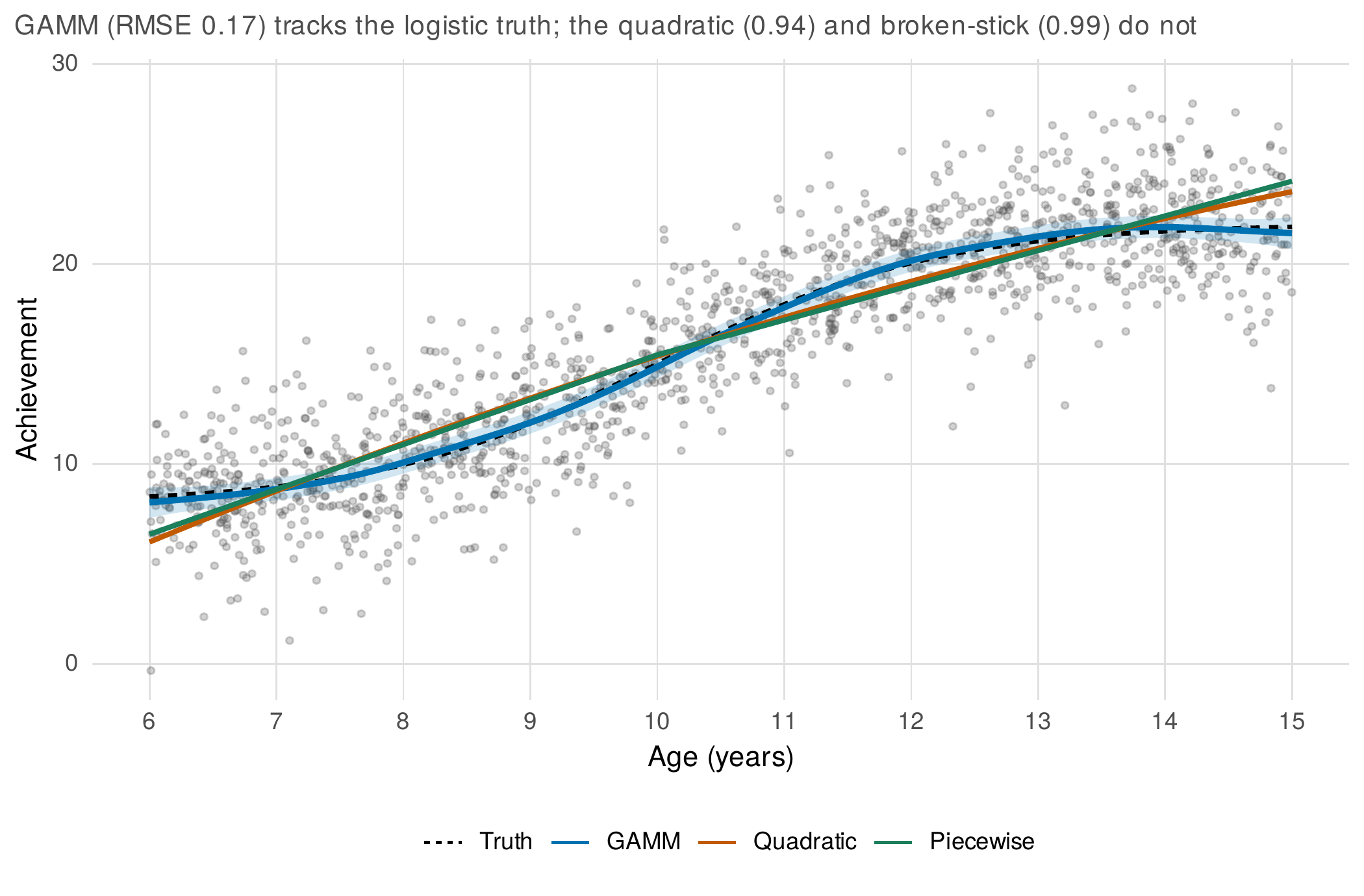
Note. Achievement across age in the growth_gam data. The generalized additive mixed model (blue, with confidence band) tracks the logistic truth (dashed) with a root-mean-squared error of \(0.17\); the quadratic (orange) and the broken-stick model (green) are forced to curve where the truth is flat and to straighten where it is steep, missing by \(0.95\) and \(0.99\). The smooth’s confidence band widens where the data are sparse, an honesty the parametric fits, which report the same narrow interval everywhere, cannot offer.
A small number of practical settings govern whether a generalized additive mixed model behaves, and Table 30.2 collects them with their rationale. The recurring principles are that the basis size is a ceiling to be set generously and checked rather than tuned, that restricted maximum likelihood is the smoothing-parameter method most resistant to overfitting, and that term selection can be turned on to let a smooth shrink to zero when a predictor earns no shape at all.
Table 30.2. Practical Settings for Fitting Generalized Additive Mixed Models in mgcv
| Setting | Recommendation | Rationale |
|---|---|---|
Basis size k | Set generously; raise if gam.check flags it | A ceiling on flexibility, not the flexibility itself; the penalty does the smoothing |
method="REML" | Default for smoothing-parameter selection | More resistant to overfitting than generalized cross-validation; stable |
select=TRUE | Use when a smooth might be null | Adds a penalty on the null space so a term can shrink to exactly zero |
bs="fs" / bs="re" | Person-smooths / random effects | The mixed-model terms; one shared penalty regularizes person curves |
bam(discrete=TRUE) | For large (EMA-scale) data | Orders-of-magnitude faster and lighter than gam/gamm |
gam.check / k.check | Always run and report | Detects a binding basis ceiling that oversmooths silently |
Note. The settings encode one doctrine: make the basis large enough that the ceiling does not bind, let restricted maximum likelihood choose the flexibility, verify the choice with the basis-dimension check, and reach for bam when the data are large. Term selection (select=TRUE) is the flexible-model counterpart of variable selection, allowing a smooth to vanish rather than fit a spurious shape.
Population smooths capture the average trajectory, but the longitudinal question is usually about heterogeneity, and the factor-smooth basis provides the nonparametric analogue of Chapter 14’s random slopes. A model with a population smooth of age plus a factor-smooth of age by child gives every child a smooth trajectory of their own, all sharing a single smoothing parameter so that individual curves borrow strength from the population and from one another rather than overfitting each child’s handful of observations. Figure 30.3 shows the gallery for forty children: each thin curve is a person’s nonparametric trajectory, wiggling around the red population smooth by as much as the shared penalty permits. This is the flexible sibling of the random-slope growth model, appropriate when the theory does not specify a functional form for individual change and when the data per person are too few to estimate a free curve for each. The residual-autocorrelation caution of Chapter 14 transfers intact: within-person residuals from a smooth are typically correlated, and if the correlation is of interest it can be modeled with an autoregressive structure through gamm, but the confounding warning stands, because a flexible smooth of time and an autoregressive residual compete to explain the same within-person dependence, and letting both float without examination can leave the model unidentified in practice.
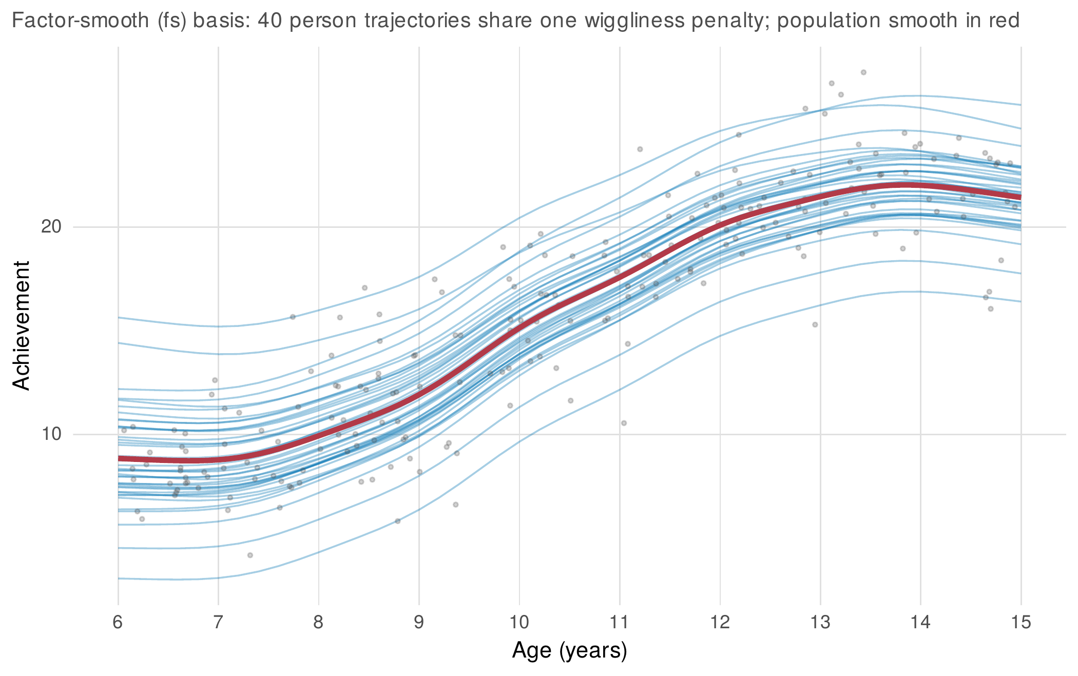
Note. Forty children’s individual smooth trajectories (thin) from a factor-smooth ("fs") basis, with the population smooth in red and raw observations in grey. Each person’s curve is nonparametric but shares one smoothing parameter with all the others, so individual trajectories are regularized toward the population shape rather than fitted freely. This is the flexible counterpart of the random-slope growth model of Chapter 14, for use when no functional form is assumed for individual change.
The comparison of groups is where flexible curves deliver an estimand parametric models struggle to express: not whether two groups differ on average but where in time they differ. The difference smooth fits a separate curve for each group and estimates their difference as a function of the predictor, and its inference must account for the fact that the difference is a whole curve rather than a single number. A pointwise confidence band, the estimate plus or minus about two standard errors at each time, has the correct coverage at any one time but understates the uncertainty of the curve as a whole, because a curve that stays inside its pointwise band at every one of many times is improbable under the band’s own logic. The simultaneous confidence band corrects this by widening the interval to the multiplier that a whole-curve excursion requires, computed by simulating from the posterior of the coefficients and taking the distribution of the maximum standardized deviation across the curve. For the tvem_rct data, a two-arm trial in which the treatment effect is built to emerge and then partly wane, the simultaneous band uses a multiplier of about \(2.5\) rather than the pointwise \(1.96\), and the difference between the arms is significant, in the simultaneous sense, across weeks six through twenty. Figure 30.4 shows the difference smooth with both bands and the significant window, and the foundations box sketches the construction.
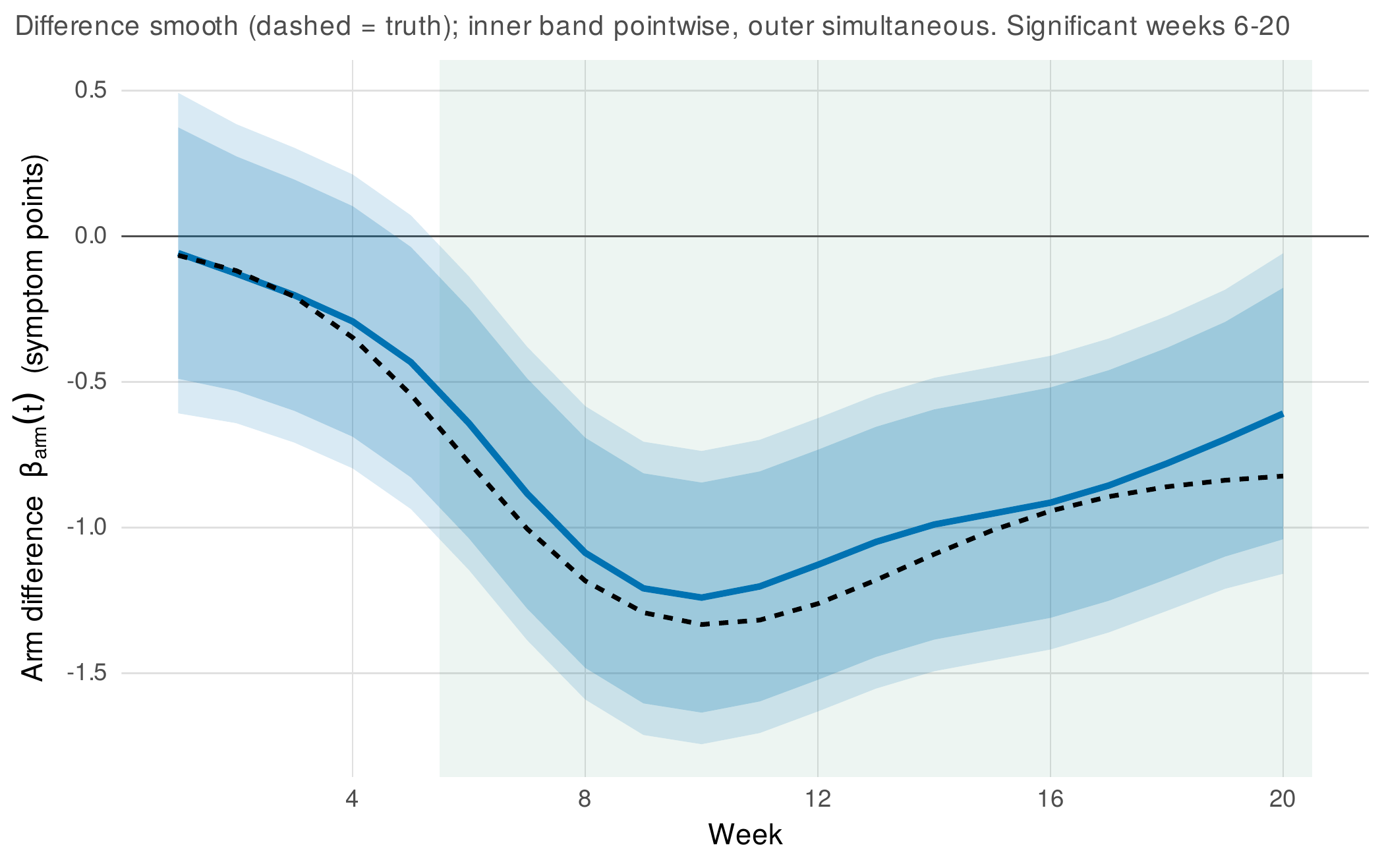
Note. The arm difference in the tvem_rct data as a function of week, with the known truth dashed. The inner band is pointwise (multiplier \(1.96\)); the outer band is simultaneous (multiplier about \(2.5\)), the correct band for asking where across the whole curve the arms differ. The difference is significant in the simultaneous sense across the shaded window, weeks six through twenty. The estimand, the location and timing of a group difference, is one a single contrast cannot express.
Foundations Box • Simultaneous bands by posterior simulation
Let \(\hat{f}(t)=X_t\hat{\boldsymbol\beta}\) be a fitted curve with coefficient covariance \(V_\beta\), so the pointwise standard error is \(s(t)=\sqrt{X_t V_\beta X_t'}\). A pointwise band is \(\hat{f}(t)\pm 1.96\,s(t)\), correct at each \(t\) but not for the curve. To build a band correct simultaneously over the whole curve, draw many coefficient vectors \(\boldsymbol\beta^{(m)}\) from the posterior \(N(\hat{\boldsymbol\beta}, V_\beta)\), form the standardized deviation curve \(|X_t(\boldsymbol\beta^{(m)}-\hat{\boldsymbol\beta})|/s(t)\), and record its maximum over \(t\). The \((1-\alpha)\) quantile of these maxima is the multiplier \(c\); the simultaneous band is \(\hat{f}(t)\pm c\,s(t)\). Because \(c\) exceeds \(1.96\), the simultaneous band is wider, and it is the honest band for the question “over what range does the curve differ from zero,” the question a difference smooth or a time-varying coefficient is usually asked.
Cyclic phenomena are the last of the section’s longitudinal applications and the point of contact with Chapter 23. A diurnal rhythm, a mood that falls toward midday and rises again by evening, is periodic, and a cyclic spline enforces that the fitted curve and its slope match at the ends of the cycle, so the rhythm joins smoothly rather than jumping from the last hour to the first. The diurnal_ema data carry such a rhythm, and Figure 30.5 fits it two ways: a cyclic spline, which spends about five effective degrees of freedom and follows the arch closely, and the single trigonometric pair of Chapter 23, a sine and a cosine at the daily frequency, which spends exactly two and captures the gross shape but cannot bend to the arch’s asymmetries. The trade-off is the chapter’s recurring one. The trigonometric pair is parametric, interpretable as an amplitude and a phase, and efficient when the rhythm is close to sinusoidal; the cyclic spline is flexible, faithful to departures from a pure sinusoid, and the safer choice when the rhythm’s shape is itself in question. Neither dominates, and the decision belongs to whether the shape of the cycle or a summary of its amplitude is the scientific target.
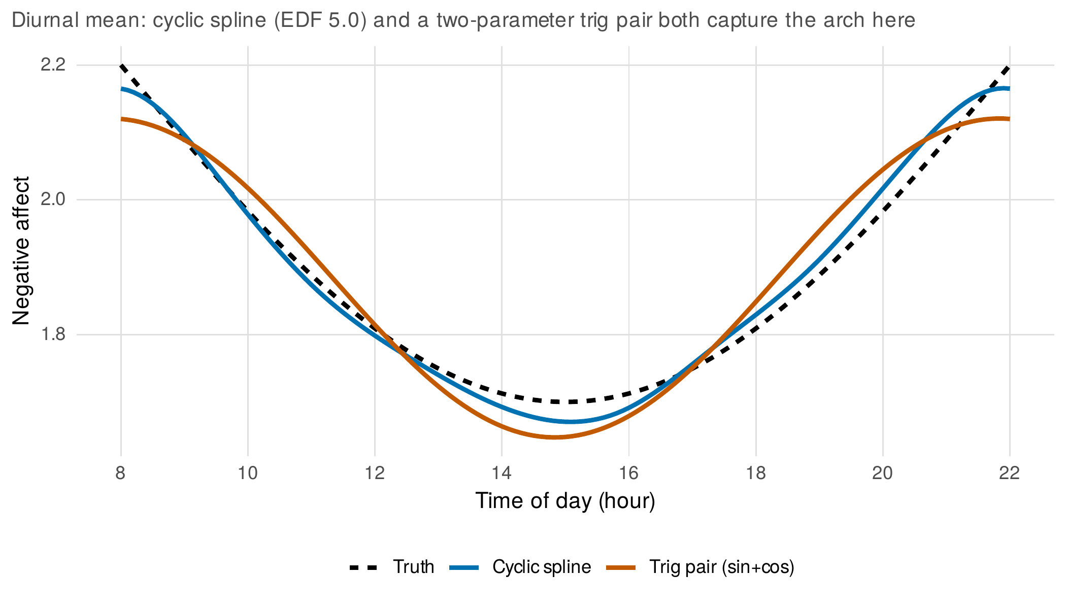
Note. The population diurnal mean of negative affect in the diurnal_ema data (dashed truth). The cyclic spline (blue, about five effective degrees of freedom) follows the arch faithfully, including its slight asymmetry; the single trigonometric pair (orange, two parameters) captures the gross rhythm but is constrained to a pure sinusoid and misses the endpoints. The cyclic spline buys fidelity with flexibility; the trigonometric pair buys interpretability with rigidity.
Software Note • Two routes, and scaling to intensive data
The choice between mgcv’s routes is practical. gamm fits through nlme and gives access to correlated-residual structures such as corAR1, at the cost of speed and of occasional convergence trouble when the random-effects and correlation structures are both rich. gam with bs="re" and bs="fs" fits the same models by penalized likelihood, is faster, and returns cleaner uncertainty for the smooths, but treats correlation only through the smooths and random effects themselves. For the large data sets of ecological momentary assessment, tens of thousands of rows, bam with discrete=TRUE and method="fREML" reduces memory and time by orders of magnitude and is the practical default; the person-specific and habituation models in this chapter’s analysis use it. The visualization packages gratia and itsadug streamline plotting and difference-smooth extraction from fitted mgcv objects; where they are unavailable the same displays are built by predicting on a grid with standard errors and simulating the simultaneous bands directly, as the companion scripts do.
30.3 Time-Varying Effect Models
The models to this point have made the shape of an outcome flexible. A time-varying effect model makes the shape of a coefficient flexible, and the shift in the question is genuine. Instead of asking how an outcome changes over time, it asks how the effect of a predictor changes over time: whether the association between stress and negative affect strengthens or weakens across adolescence, whether the grip of craving on relapse loosens across a quit attempt, whether a treatment’s benefit emerges gradually and then fades. The specification is the varying-coefficient model of Hastie and Tibshirani (1993): the coefficient on a predictor is itself a smooth function of time, \(y = \cdots + \beta(t)\,x + \cdots\), with \(\beta(t)\) a penalized spline. In mgcv the varying coefficient is written s(time, by = x), a smooth of time multiplied by the covariate \(x\), and the dedicated tvem package from the Methodology Center lineage wraps the same idea with conveniences for intensive longitudinal data. The reading of the output is a curve, not a coefficient, and its band is the simultaneous band of the previous section, because the question is again about a whole curve.
The chapter’s signature figure recovers two time-varying effects of different kinds. In the tvem_rct data the treatment effect \(\beta_{\text{arm}}(t)\) is built to be near zero at the start, to emerge around week six, to peak near week eleven at a reduction of about \(1.3\) symptom points, and to wane partly by week twenty; the varying-coefficient model recovers this curve with a root-mean-squared error of \(0.10\), placing the emergence at week six and the peak at week ten, essentially the truth. In the diurnal_ema data the within-person coefficient linking momentary stress to momentary negative affect is built to habituate, declining smoothly from about \(0.65\) on the first study day to about \(0.30\) by the fourteenth as the person adapts to the monitoring and to the stressors; the model recovers the decline almost exactly, from \(0.65\) to \(0.29\). Figure 30.6 shows both. The two panels make the generality of the idea concrete: a coefficient can vary along the time axis of a treatment or along the time axis of a study, and in each case the deliverable is a curve with a band that says when the effect is present and how it moves.
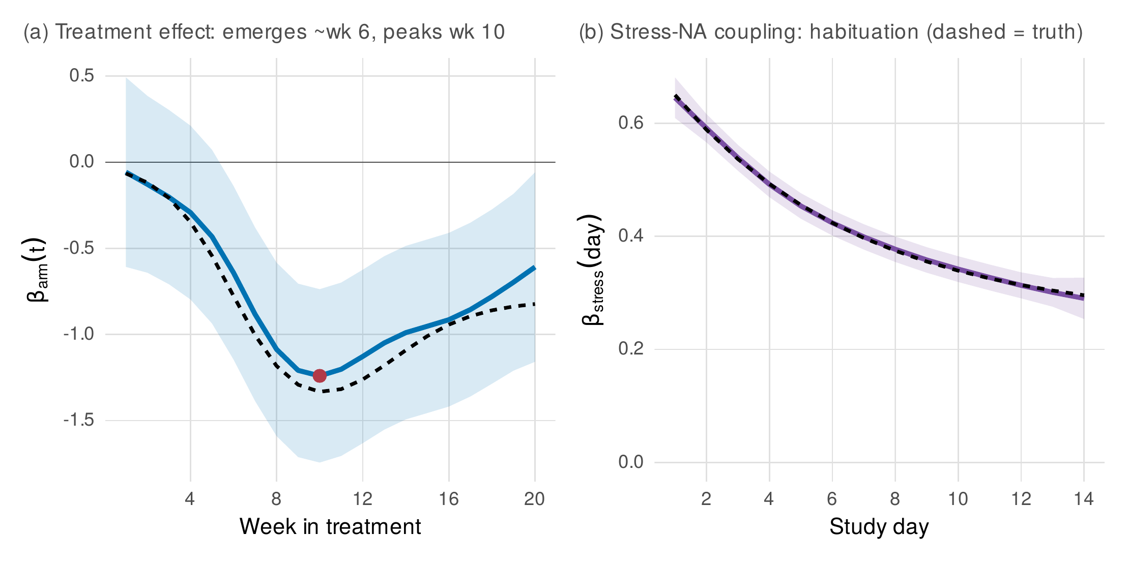
Note. Panel (a): the treatment effect \(\beta_{\text{arm}}(t)\) in the tvem_rct data (blue, with simultaneous band; dashed truth) emerges near week six and peaks near week ten (dot), then wanes, a trajectory a single hazard ratio or mean contrast cannot express. Panel (b): the within-person stress-to-negative-affect coefficient \(\beta_{\text{stress}}(\text{day})\) in the diurnal_ema data (purple; dashed truth) habituates across the study, declining from about \(0.65\) to \(0.30\). In both, the estimand is the shape of an effect over time.
The distinction that keeps time-varying effect models from being oversold is that a parametric interaction with time is a special case of a time-varying effect, not an equivalent of it. Entering an \(x\)-by-time product term lets the effect of \(x\) change linearly with time, which is a time-varying effect constrained to a straight line; the varying-coefficient model relaxes that constraint and lets the effect take whatever smooth shape the data support, so it can find an effect that emerges and wanes, which no single product term can. The implication is directional: whenever a linear interaction with time is fit, a time-varying effect model nests it and tests whether the linearity holds, and a time-varying effect that turns out straight simply reproduces the interaction with honest uncertainty about its linearity. Table 30.3 places the method among its neighbors. The frontier the section flags honestly is the multilevel time-varying effect model, in which the time-varying coefficient itself varies across persons, \(\beta_i(t)\); approaches exist, combining factor-smooths with by-variables, but the estimation is delicate and the literature is still settling, so a claim about person-specific time-varying effects should be made cautiously and checked against the current methodological work.
Table 30.3. What Four Flexible-Curve Frameworks Answer
| Framework | Unit and question | Choose when |
|---|---|---|
| Parametric growth (Ch. 14, 19) | A named curve of the outcome; its parameters | Theory pins the functional form; interpretability is paramount |
| GAMM (this ch.) | A flexible curve of the outcome; its shape | The shape is unknown or nonstandard; honest bands are needed |
| TVEM (this ch.) | A flexible curve of a coefficient; when a predictor matters | The effect of a predictor may change over time |
| FDA (this ch.) | The whole curve as datum; modes of curve variation | Dense curves per unit; registration or curve-level inference is the goal |
Note. The frameworks are ordered by what plays the role of the unit of analysis: a parameter, an outcome curve, a coefficient curve, or a whole function. A parametric interaction with time is a constrained special case of a time-varying effect model; functional principal components are the functional analogue of growth factors (Table 30.4). The choice is driven by the scientific target, not by which fits best.
Common Pitfall • Reading a flexible model too eagerly
A wiggle inside the band is not a finding. A smooth that dips at week six has not established a phenomenon at week six unless the band excludes the no-dip curve there; narrate only features the simultaneous band supports. A basis too small oversmooths silently. If \(k\) is set below the shape’s complexity the penalty cannot recover it and the misfit is invisible without gam.check; treat \(k\) as a ceiling and check that it does not bind. A time-varying effect is not moderation by a measured variable. \(\beta(t)\) says the effect changes with time, not that time causes the change; a third variable moving with time can drive both. A smooth of time beside an autoregressive residual double-counts within-person dependence. Decide which structure carries the dependence and examine, rather than assume, that the two are not competing.
30.4 Functional Data Analysis: A Working Introduction
Functional data analysis makes a conceptual move that reframes everything: the datum is not a scalar or a vector but an entire curve, \(y_i(t)\), one function per person. A study of diurnal mood yields not a table of beeps but a sample of daily mood curves; a study of movement yields a sample of trajectories; a study of physiology yields a sample of signals. Two routes lead into the curve. The smoothing-first route represents each curve in a basis and treats the smoothed function as the object of analysis, which is the classical functional-data stance; the model-based route, the generalized additive mixed model of Section 30.2, reaches many of the same ends by modeling the pointwise data with smooths and random effects. The two agree often enough that a working researcher can treat the generalized additive mixed model as sufficient for most longitudinal questions and reserve the full functional apparatus for when its distinctive tools are needed. The first such tool is registration.
Registration confronts a problem invisible to pointwise methods. When curves share a shape but differ in the timing of its features, a peak that arrives early for some units and late for others, the pointwise average blurs the peak into a low broad hump that resembles no individual curve, because at each time it averages units that are at different points in their shared trajectory. The distinction is between amplitude variation, differences in the height of a feature, and phase variation, differences in its timing, and separating them is the work of registration (Marron et al., 2015). Figure 30.7 demonstrates it on a bundle of curves that share a single peak of varying height and varying location. The unaligned average, in red on the left, is smeared and low; landmark registration, which warps each curve’s time axis to bring its peak to the common location, reduces the standard deviation of peak timing from \(0.095\) to \(0.010\) and restores a mean, in red on the right, that regains the sharp peak every individual curve possesses. The registered curves and the warping functions then become separate objects of analysis: the aligned curves carry the amplitude variation, and the warps carry the phase variation, each analyzable in its own right. Where the timing of events is itself substantive, as in the alignment of physiological responses or the tempo of a developmental sequence, registration is indispensable, and no amount of pointwise smoothing substitutes for it.
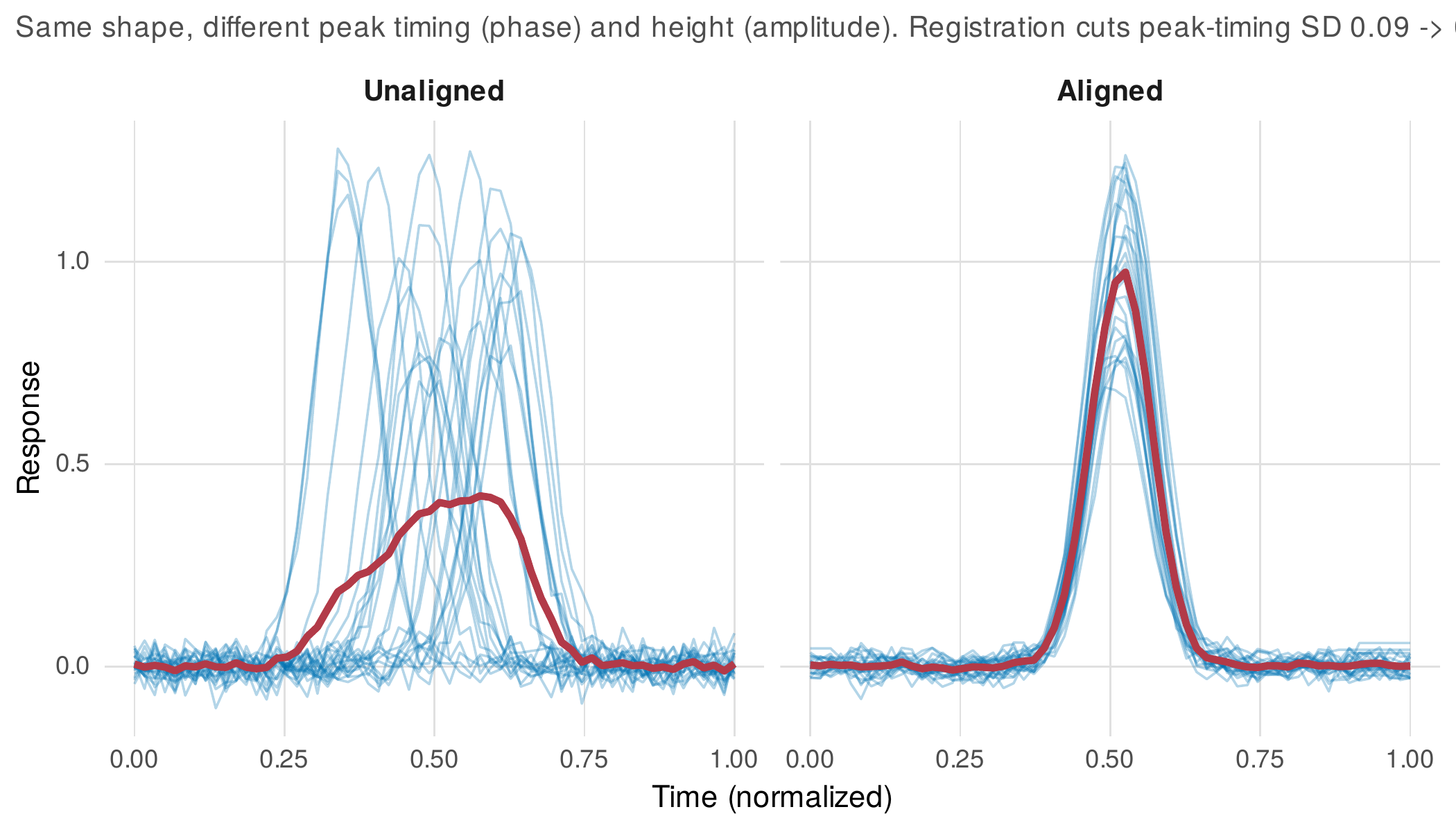
Note. Curves that share a peak of varying height (amplitude) and varying timing (phase). Left: unaligned, the pointwise mean (red) is smeared into a low hump that matches no individual curve. Right: after landmark registration to a common peak location, the standard deviation of peak timing falls from \(0.095\) to \(0.010\) and the mean (red) recovers the sharp peak. Averaging before registration destroys exactly the feature the curves share; pointwise methods cannot see the phase variation that registration removes.
The second distinctive tool is functional principal component analysis, and it is the functional analogue of the growth factors of Chapter 19. A growth model summarizes each person’s trajectory by a few latent factors, an intercept and a slope, that are common shapes with person-specific weights; functional principal component analysis summarizes each person’s curve by a few functional principal components, empirically estimated common shapes, the modes of variation, with person-specific scores. The modes are the eigenfunctions of the curve covariance, ordered by the variance they explain, and the scores are each person’s loadings on them, mean-zero features that can be analyzed like any person-level variable. Applied to the diurnal profiles of the diurnal_ema data, which are generated from three planted modes, the analysis recovers them cleanly: the leading component, explaining sixty-eight percent of the between-person variance against a planted sixty-five, is a level shift, a nearly flat eigenfunction that raises or lowers the whole day; the second, twenty percent against twenty-five, is a morning-to-evening tilt; the third, nine percent against eleven, is a midday curvature that deepens or fills the midday dip. The recovered person scores correlate with the true planted scores at \(0.999\), \(0.995\), and \(0.986\). Figure 30.8 shows the modes as perturbations of the mean and the scores as person features, and Table 30.4 makes the correspondence with growth factors explicit. The scores then serve wherever growth factors serve: as outcomes regressed on covariates, as predictors of later events, or as the person-level summary in a two-stage analysis, and function-on-scalar regression generalizes the idea by regressing whole curves on covariates directly.
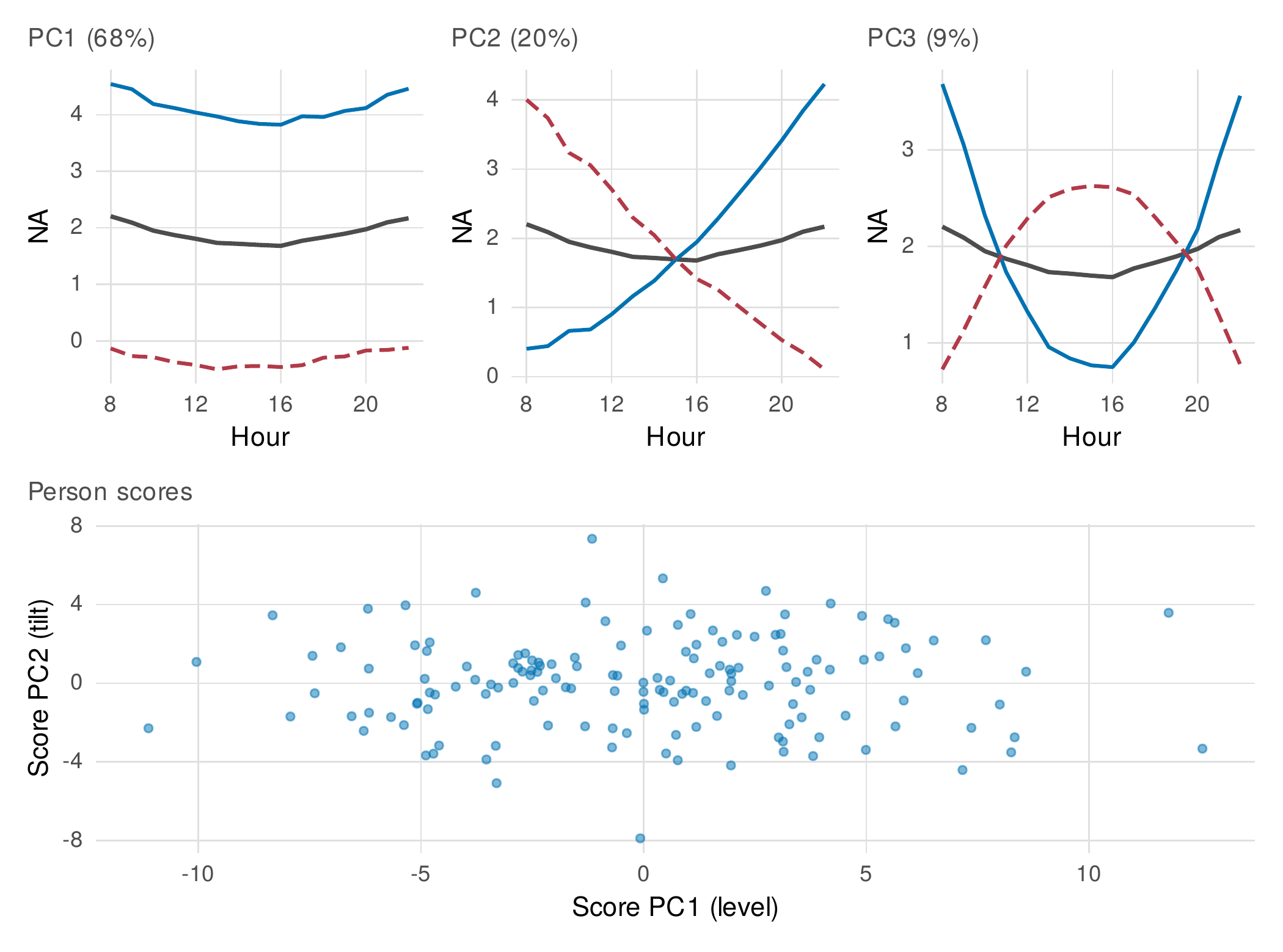
Note. The top row shows the three leading functional principal components of the diurnal_ema profiles as perturbations of the mean curve (grey): adding (blue) and subtracting (dashed red) each mode. The first (sixty-eight percent of between-person variance) is a level shift, the second (twenty percent) a morning-to-evening tilt, the third (nine percent) a midday curvature. The bottom panel plots the person scores on the first two modes, mean-zero features usable like growth factors. Recovered scores correlate with the planted truth above \(0.98\).
Table 30.4. Growth Factors and Functional Principal Components
| Growth model (Ch. 19) | Functional PCA | Shared idea |
|---|---|---|
| Fixed basis (intercept, slope, quadratic) | Estimated eigenfunctions (modes of variation) | Common shapes |
| Factor loadings (fixed) | Eigenfunction values over \(t\) | How a shape maps onto time |
| Factor scores (random, per person) | Component scores (per person) | Person-specific weights |
| Factor variances | Eigenvalues | Variance each shape explains |
| Model-imposed shapes | Data-driven shapes | Parametric vs empirical |
Note. Functional principal component analysis is growth-factor thinking with the shapes estimated from the data rather than imposed by the model. The scores are the functional counterpart of factor scores and are used identically: as outcomes, predictors, or person-level summaries. The price of the data-driven shapes is that they are descriptive modes of variation, not theoretically named factors, and require interpretation.
When does the functional machinery earn its cost over a generalized additive mixed model that would answer the same substantive question with familiar tools? The functional apparatus pays when the data are densely functional, many measurements per unit tracing a genuine curve, as in physiology, accelerometry, eye-tracking, or mouse-tracking; when registration is needed because the timing of features varies across units and is itself of interest; and when the inference is about whole curves, their modes of variation or their regression on covariates, rather than about a population mean trajectory. It does not pay, and a generalized additive mixed model suffices, when the data are sparse per unit, when the question is about an average trajectory or a group difference, and when the timing of features is fixed by design. The sparse case deserves a caveat against a common misconception: functional principal component analysis does not require dense, equally spaced grids, because the sparse-data methods of Yao, Müller, and Wang (2005) estimate the modes from the pooled covariance of irregular observations, which makes the machinery available even to the ragged sampling of ecological momentary assessment.
30.5 Preventing the Abuses of Flexibility
Flexible models fail in characteristic ways, and the discipline of using them is largely the discipline of forestalling those failures. The first is concurvity, the smooth world’s collinearity: when two predictors entered as separate smooths are near-functionally related, so that one is nearly a smooth function of the other, their smooths are jointly unidentified and swing to large, mutually cancelling shapes that fit the data equally well in combination but mean nothing separately. Figure 30.9a shows the pathology, with two smooths of nearly dependent predictors bowing in opposite directions under wide bands; mgcv’s concurvity function flags it, returning a worst-case index near one, its maximum, for this pair. The remedy is not a better penalty but a better model: drop one of the redundant predictors, or combine them, because no amount of smoothing recovers a distinction the data do not contain. The second failure is the narration of noise. A smooth fit aggressively enough to a small or noisy sample will invent structure, and the danger is not the wiggle itself but the story told about it. Figure 30.9b fits an undersmoothed curve to data with no signal at all, a flat truth, and the fit obligingly produces dips and humps with pointwise bands that seem to support them; the discipline is to read the simultaneous band, which here contains the flat line throughout, and to refuse the narrative the pointwise band invites.
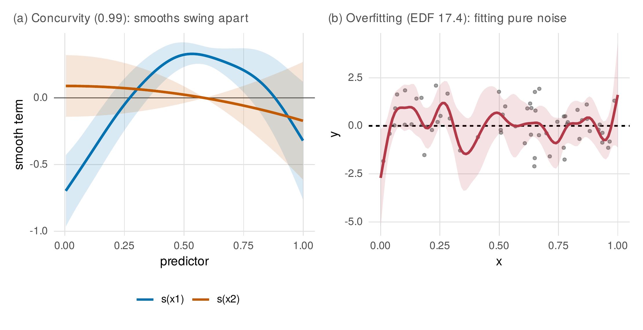
Note. Panel (a): concurvity. Two smooths of nearly functionally dependent predictors (worst-case index \(0.99\)) swing to large opposing shapes that cancel; separately they are meaningless, and the fix is to drop or combine a predictor, not to smooth harder. Panel (b): overfitting. An undersmoothed curve fit to pure noise (a flat truth, dashed) invents dips and peaks that its pointwise band appears to license; the simultaneous band contains the flat line everywhere, and the wiggles are not to be narrated.
The remaining abuses are matters of hygiene that a reporting standard enforces. Extrapolation beyond the range of the data is unsupported for a smooth exactly as for a polynomial, and more insidiously so, because a penalized smooth reverts to its unpenalized null-space behavior, typically linear, outside the data and can appear deceptively confident there. The basis-dimension diagnostic must be run and reported, because an undersized basis oversmooths without warning. The smoothing-parameter selection method should be stated, because generalized cross-validation and restricted maximum likelihood can differ, with restricted maximum likelihood the more resistant to overfitting and the current default recommendation. And the distinction between what was fixed and what was data-chosen must be preserved for a flexible model to be preregisterable at all: a preregistration can fix the basis type, the maximum basis size, the smoothing-parameter method, and the inferential band, leaving only the shape itself to the data, which is exactly the division of labor that makes penalized regression confirmatory rather than exploratory. Table 30.5 collects the reporting elements, and the practice box addresses the computational realities of applying these models at the scale intensive designs now reach.
Table 30.5. Reporting Checklist for Flexible-Curve Models
| Element | What to report |
|---|---|
| Basis and size | Basis type per smooth and the maximum basis size \(k\); the ceiling, not the realized flexibility |
| Effective df | The estimated effective degrees of freedom per smooth (the shape earned) |
| Smoothing method | Restricted maximum likelihood (preferred) or generalized cross-validation |
| Basis-check | The gam.check \(k\)-index and its verdict for each smooth |
| Bands | Pointwise or simultaneous, and how simultaneous bands were constructed |
| Random structure | Random effects, factor-smooths, and any residual correlation model |
| Fixed vs chosen | What the analysis fixed a priori and what it let the data determine |
Note. Reporting the maximum basis size and the realized effective degrees of freedom separately is the flexible-model analogue of reporting the model and its fit; the first is the ceiling the analyst set, the second is the shape the data bought. Stating what was fixed a priori (basis, size, smoothing method, band type) against what was data-chosen (the shape) is what allows a penalized-spline analysis to be preregistered.
In Practice • Flexible models at intensive-data scale
Ecological momentary assessment produces data sets of tens or hundreds of thousands of rows, and the naive gamm fit will exhaust memory or time. The bam function with discrete=TRUE bins covariate values and exploits the structure to fit in seconds what gam would take minutes or hours to fit, with method="fREML" the stable default; the person-specific and habituation models in this chapter’s analysis use exactly this. When factor-smooths over thousands of persons are needed, the shared smoothing parameter keeps the parameter count manageable, but the memory still grows with the number of persons, and subsampling persons for exploratory fits before the full run is prudent. The choice between gamm and gam with random-effect bases is partly a convergence question: the penalized-likelihood route (gam, bam) is more robust when the random structure is rich, while gamm is the route when a specific residual correlation must be modeled.
Chapter Summary
Flexible-curve methods let the data determine the shape of change while keeping inference honest, and they are continuous with the mixed-model thinking of the whole book rather than a departure from it. A penalized spline writes a curve as a weighted sum of basis functions and disciplines the fit with a wiggliness penalty whose strength, the smoothing parameter, is a bias-variance dial chosen from the data by restricted maximum likelihood; the effective degrees of freedom report how much shape the data earned. The deep fact is that a smooth is a random effect and the smoothing parameter is a variance ratio, so generalized additive mixed models estimate smooths and random effects in one framework. On the growth_gam data a penalized smooth recovers a logistic growth spurt a quadratic and a broken-stick model badly miss, factor-smooths give every child a nonparametric trajectory regularized toward the population, and a difference smooth with a simultaneous band locates where two arms diverge, weeks six through twenty, an estimand a single contrast cannot express. Cyclic splines model rhythms flexibly where the trigonometric pair of Chapter 23 models them parametrically, and the choice turns on whether the shape or a summary of the cycle is the target. Time-varying effect models make a coefficient a smooth function of time, answering when a predictor matters: on the tvem_rct data the treatment effect is recovered as a curve that emerges near week six and peaks near week ten, and on the diurnal_ema data the stress-to-affect coupling is recovered as a habituating decline from about \(0.65\) to \(0.30\); a parametric interaction with time is a straight-line special case that these models nest and test. Functional data analysis treats the whole curve as the datum: registration separates amplitude from phase and rescues a mean that pointwise averaging destroys, and functional principal components are the empirical analogue of growth factors, recovering level, tilt, and midday-curvature modes of diurnal profiles with scores that correlate with the truth above \(0.98\). The functional machinery earns its cost for dense curves, registration needs, and curve-level inference; a generalized additive mixed model suffices otherwise. The abuses are characteristic and preventable: concurvity unidentifies near-dependent smooths, aggressive smoothing narrates noise a simultaneous band refutes, extrapolation is unsupported, and the discipline of reporting the basis, the effective degrees of freedom, the smoothing method, the basis check, and the band, and of distinguishing what was fixed from what was data-chosen, is what makes a flexible model confirmatory rather than a license to see shapes in noise.
Bringmann, L. F., Hamaker, E. L., Vigo, D. E., Aubert, A., Borsboom, D., & Tuerlinckx, F. (2017). Changing dynamics: Time-varying autoregressive models using generalized additive modeling. Psychological Methods, 22(3), 409–425. https://doi.org/10.1037/met0000085
Dziak, J. J., Li, R., Tan, X., Shiffman, S., & Shiyko, M. P. (2015). Modeling intensive longitudinal data with mixtures of nonparametric trajectories and time-varying effects. Psychological Methods, 20(4), 444–469. https://doi.org/10.1037/met0000048
Eilers, P. H. C., & Marx, B. D. (1996). Flexible smoothing with B-splines and penalties. Statistical Science, 11(2), 89–121. https://doi.org/10.1214/ss/1038425655
Goldsmith, J., Scheipl, F., Huang, L., Wrobel, J., Gellar, J., Harezlak, J., McLean, M. W., Swihart, B., Xiao, L., Crainiceanu, C., & Reiss, P. T. (2024). refund: Regression with functional data (R package version 0.1-40) [Computer software]. https://CRAN.R-project.org/package=refund
Hastie, T., & Tibshirani, R. (1993). Varying-coefficient models. Journal of the Royal Statistical Society: Series B (Methodological), 55(4), 757–796. https://doi.org/10.1111/j.2517-6161.1993.tb01939.x
Marron, J. S., Ramsay, J. O., Sangalli, L. M., & Srivastava, A. (2015). Functional data analysis of amplitude and phase variation. Statistical Science, 30(4), 468–484. https://doi.org/10.1214/15-STS524
Pedersen, E. J., Miller, D. L., Simpson, G. L., & Ross, N. (2019). Hierarchical generalized additive models in ecology: An introduction with mgcv. PeerJ, 7, Article e6876. https://doi.org/10.7717/peerj.6876
Ramsay, J. O., Hooker, G., & Graves, S. (2009). Functional data analysis with R and MATLAB. Springer. https://doi.org/10.1007/978-0-387-98185-7
Ramsay, J. O., & Silverman, B. W. (2005). Functional data analysis (2nd ed.). Springer. https://doi.org/10.1007/b98888
Ruppert, D., Wand, M. P., & Carroll, R. J. (2003). Semiparametric regression. Cambridge University Press. https://doi.org/10.1017/CBO9780511755453
Shiyko, M. P., Lanza, S. T., Tan, X., Li, R., & Shiffman, S. (2012). Using the time-varying effect model (TVEM) to examine dynamic associations between negative affect and self confidence on smoking urges: Differences between successful quitters and relapsers. Prevention Science, 13(3), 288–299. https://doi.org/10.1007/s11121-011-0264-z
Sørensen, Ø., Walhovd, K. B., & Fjell, A. M. (2021). A recipe for accurate estimation of lifespan brain trajectories, distinguishing longitudinal and cohort effects. NeuroImage, 226, Article 117596. https://doi.org/10.1016/j.neuroimage.2020.117596
Tan, X., Shiyko, M. P., Li, R., Li, Y., & Dierker, L. (2012). A time-varying effect model for intensive longitudinal data. Psychological Methods, 17(1), 61–77. https://doi.org/10.1037/a0025814
van Rij, J., Wieling, M., Baayen, R. H., & van Rijn, H. (2020). itsadug: Interpreting time series and autocorrelated data using GAMMs (R package version 2.4) [Computer software]. https://CRAN.R-project.org/package=itsadug
Wood, S. N. (2004). Stable and efficient multiple smoothing parameter estimation for generalized additive models. Journal of the American Statistical Association, 99(467), 673–686. https://doi.org/10.1198/016214504000000980
Wood, S. N. (2011). Fast stable restricted maximum likelihood and marginal likelihood estimation of semiparametric generalized linear models. Journal of the Royal Statistical Society: Series B (Statistical Methodology), 73(1), 3–36. https://doi.org/10.1111/j.1467-9868.2010.00749.x
Wood, S. N. (2017). Generalized additive models: An introduction with R (2nd ed.). Chapman & Hall/CRC. https://doi.org/10.1201/9781315370279
Yao, F., Müller, H.-G., & Wang, J.-L. (2005). Functional data analysis for sparse longitudinal data. Journal of the American Statistical Association, 100(470), 577–590. https://doi.org/10.1198/016214504000001745