Chapter 31
Machine Learning and Data-Driven Exploration for Longitudinal Data
Machine learning enters a methods book for psychologists neither as a savior nor as a threat but as a set of tools whose value is decided, like any tool’s, by the question it answers and the errors it avoids. The chapter takes that stance and holds it. It begins by separating prediction from explanation, the two research goals Breiman named cultures, because a method optimized to forecast a new person’s relapse is judged by different evidence than a model built to explain why relapse occurs, and confusing the two produces the characteristic pathologies of applied machine learning: a black box praised for insight it cannot provide, or a beautiful causal story with no predictive skill. The load-bearing section is the one on honest evaluation, because the single most consequential fact about longitudinal machine learning is that the resampling schemes taught for independent data leak when the rows are repeated measures of the same persons. A model tested by randomly splitting rows is tested partly on people it has already seen, and the accuracy it reports is inflated in a way no amount of algorithmic sophistication corrects. The chapter demonstrates the leak numerically and then builds the resampling discipline that repairs it: grouping folds by person to estimate how well a model generalizes to new people, and chaining folds through time to estimate how well it forecasts a person’s future, each matched to the prediction task it honestly evaluates, and each measured against the humblest baseline of all, yesterday’s value. On that foundation it develops the methods that do longitudinal work: mixed-effects trees and forests that partition heterogeneity without ignoring nesting, trajectory clustering as the algorithmic rival to the model-based mixtures of Chapter 22, regularization for the many-predictor problems that intensive designs create, and idiographic forecasting where the pooling lesson of Chapter 25 returns in predictive clothing. Throughout, the discipline established in the evaluation section is inherited by every method that follows.
Learning Objectives
After working through this chapter, you should be able to: (1) distinguish prediction, description, and explanation as research goals and identify which a longitudinal question requires; (2) design resampling that respects dependence, choosing person-grouped cross-validation to estimate new-person generalization and forward-chaining to estimate within-person forecasting, and recognize the leakage that naive row-wise splitting produces; (3) fit and interpret tree and forest methods adapted to nested data, including growth-parameter and mixed-effects trees for subgroup discovery; (4) run algorithmic trajectory clustering and articulate its trade-off against model-based mixtures; (5) apply regularization to many-predictor longitudinal problems with honesty about post-selection inference; (6) evaluate predictive performance with appropriate metrics, calibration, and mandatory baselines including persistence; (7) interpret black-box models responsibly with permutation importance and partial-dependence displays read as descriptive; and (8) report a predictive study to current standards, distinguishing what was fixed in advance from what the data determined.
31.1 Two Cultures, One Researcher
Breiman (2001) drew a line between two cultures of statistical practice. The data-modeling culture posits a stochastic model relating inputs to outputs, estimates its parameters, and interprets them; its currency is explanation, and its validity rests on the model being approximately correct. The algorithmic-modeling culture treats the data-generating mechanism as unknown and unknowable, and seeks any function, however uninterpretable, that predicts the output accurately on new data; its currency is predictive skill, and its validity rests on honest out-of-sample evaluation. Psychology has lived almost entirely in the first culture, and Yarkoni and Westfall (2017) argued that this has cost the field, that an overinvestment in explanation and a corresponding neglect of prediction has produced theories that fit existing data and forecast nothing, and that borrowing the predictive discipline of machine learning would be a corrective. The argument has force and has drawn thoughtful rebuttals, chiefly that prediction and explanation are different goals rather than competing answers to one goal, so that a field’s choice between them should follow from what it is trying to learn (Shmueli, 2010).
This book’s move is the estimand-first reconciliation it has used throughout: name the target of inference before choosing the method, and let the target dictate both the method and the standard of evidence. Some longitudinal questions are genuinely predictive. Whether a patient will relapse in the next month, which students are at risk of dropping out, when a just-in-time intervention should fire, these are questions about what will happen to a specific person, and they are answered well by a model with high out-of-sample predictive skill whether or not its internals are interpretable. Other questions are structural or causal, about why an outcome occurs or what would change it, and for these a predictive black box is beside the point. The error is not to use machine learning but to mismatch it to the question: to read variable importance as a causal effect, or to dismiss a well-validated predictive model because its coefficients lack a theoretical story. Table 31.1 maps the chapter’s methods onto the goals they serve, and Figure 31.1 draws the two cultures with the estimand-first bridge between them.
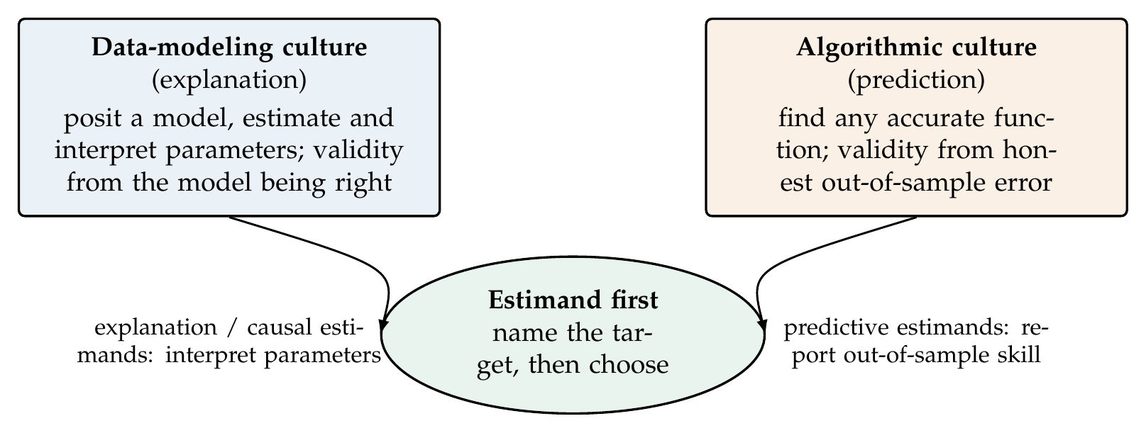
Note. Breiman’s two cultures pursue different goals: explanation through an interpretable model assumed correct, and prediction through any function validated out of sample. They are not rivals to be adjudicated but goals to be chosen between. The book’s estimand-first rule resolves the tension: decide whether the question is predictive or structural, then select the method and the standard of evidence that goal requires. The failure mode is the mismatch, reading a predictive model’s internals as explanation or judging an explanatory model by predictive skill.
Table 31.1. Research Goals and the Chapter’s Methods
| Goal | Question form | Methods and evidence |
|---|---|---|
| Prediction | What will happen to this person? | Forests, regularization, idiographic forecasting; evidence is honest out-of-sample skill vs a baseline |
| Description | What patterns are in these data? | Trajectory clustering, importance, partial dependence; evidence is stability and replication |
| Explanation | Why does the outcome occur? | Mixed-effects and SEM trees for heterogeneity; evidence is validation and theory, not fit |
Note. The same algorithm can serve different goals; a random forest can forecast (prediction) or rank features (description), but its variable importance is not a causal effect (explanation). The estimand fixes which column applies and therefore which evidence is required. Reporting predictive skill as if it demonstrated a mechanism, or a mechanism as if it guaranteed predictive skill, is the recurring category error.
31.2 Honest Evaluation with Dependent Data
The most important fact in this chapter is that the cross-validation taught for independent observations is biased for repeated measures, and the bias is optimistic. When the rows of a data set are occasions nested within persons, randomly assigning rows to folds places some of a person’s occasions in the training set and others in the test set, so the model is evaluated partly on people it has already learned. Because occasions within a person are correlated, sometimes strongly, the model that has seen a person’s other occasions predicts the held-out ones better than it would predict a genuinely new person, and the cross-validated accuracy it reports overstates the accuracy it would achieve in use. This is leakage, and it is not a subtle bias to be noted and set aside; it is the difference between a model that works in the paper and one that fails in deployment.
The demonstration uses the affect_ema data, where the task is to predict momentary negative affect from momentary predictors and a lagged outcome, and the learner is a random forest. Figure 31.2 shows the result under three resampling schemes. Naive row-wise ten-fold cross-validation, which ignores the nesting and additionally uses a person-level aggregate feature computed on the full sample, reports a test \(R^2\) of \(0.41\). Person-grouped cross-validation, which holds out whole persons so that no test person appears in training, reports \(0.35\). Forward-chaining, which trains on each person’s earlier occasions and tests on their later ones, reports \(0.35\) as well. The naive scheme is optimistic by \(0.06\) in \(R^2\), a seventeen percent relative inflation, and the gap is stable across repeated splits, which places the two estimates more than seven standard errors apart. The persistence baseline, which simply predicts that negative affect equals its previous value, reports \(0.27\), and the comparison it enables is the sobering one: the honest model beats yesterday’s value by only \(0.08\) in \(R^2\). A study that reported the naive figure would claim skill it does not have, and a study that omitted the persistence baseline would claim novelty for a model barely better than doing nothing.
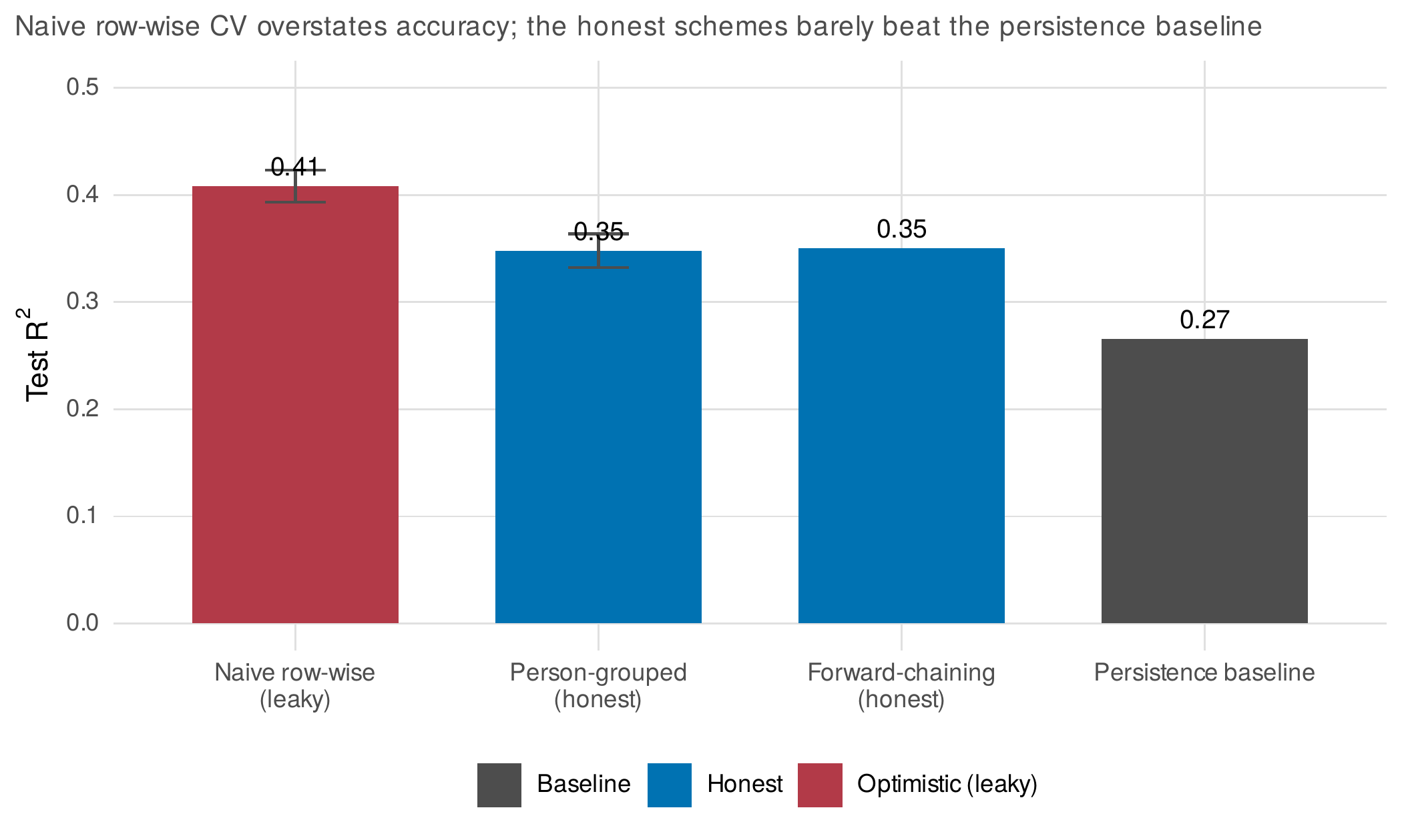
Note. Test \(R^2\) for predicting momentary negative affect in the affect_ema data under three resampling schemes and a baseline. Naive row-wise cross-validation (red) reports \(0.41\); it is optimistic because test persons also appear in training and because a person-aggregate feature was computed on the full sample. Person-grouped and forward-chaining cross-validation (blue), which respect the nesting and the arrow of time, report \(0.35\), the honest estimates. The persistence baseline (grey), predicting the previous value, reports \(0.27\): the honest model’s advantage over doing nothing is modest. Error bars are \(\pm 1.96\) standard errors over repeated splits.
The repair is to match the resampling scheme to the prediction task, and there are two tasks. Predicting a new person’s outcomes, the screening and prognosis case, is evaluated by person-grouped cross-validation, which partitions persons rather than rows into folds so that every test person is entirely unseen during training; its exchangeability argument is that new persons in the test folds stand in for the new persons the model will face in use. Predicting a person’s future from their past, the forecasting and just-in-time case, is evaluated by forward-chaining, also called rolling-origin evaluation, which for each person trains on occasions up to some time and tests on later ones, never letting the future inform the past. Table 31.2 is the selector, and Figure 31.3 draws the two schemes. Two further disciplines complete the picture. Preprocessing, any scaling, imputation, or feature construction, must happen inside the training folds only, because a transformation fit on the whole sample leaks test information into training, exactly the leak the person-aggregate feature introduced above. And when a model’s hyperparameters are tuned, the tuning must itself be cross-validated inside the training folds, a nested cross-validation, because choosing hyperparameters by test-set performance and then reporting that performance is a subtler form of testing on the training data (Varma & Simon, 2006).
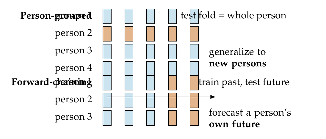
Note. Blue cells are training occasions, orange cells test occasions. Person-grouped cross-validation (top) assigns whole persons to the test fold, so no test person is seen in training; it estimates generalization to new persons. Forward-chaining (bottom) trains on each person’s earlier occasions and tests on their later ones, never using the future to predict the past; it estimates within-person forecasting. Naive row-wise splitting, not shown, scatters a person’s occasions across training and test folds and so leaks.
Table 31.2. Resampling Selector for Longitudinal Prediction
| Prediction task | Scheme | R idiom (grouped/blocked) |
|---|---|---|
| Generalize to new persons | Person-grouped \(k\)-fold | group_vfold_cv(group=person) |
| Forecast a person’s future | Forward-chaining / rolling origin | sliding_period / per-person time splits |
| Tune hyperparameters | Nested CV (inner loop) | inner group_vfold_cv within each training fold |
| Report uncertainty | Repeated CV | repeat the split; report spread |
| Never (leaks) | Naive row-wise \(k\)-fold | (do not use with repeated measures) |
Note. The scheme is chosen by the task, not by convenience. Person-grouped folds answer “how well does this predict a new person”; forward-chaining answers “how well does this forecast this person’s future.” Preprocessing and tuning belong inside the training folds. The rsample and tidymodels idioms are named for reference; their interfaces change, so verify against current documentation.
Foundations Box • Why grouped cross-validation estimates new-person error
Suppose each person \(j\) contributes a random effect \(u_j\) that shifts all of their occasions, and the goal is to predict occasions for a person not in the sample. Under naive row-wise splitting, a test occasion of person \(j\) has training occasions of the same person, from which any learner can estimate \(u_j\); the test error therefore reflects prediction with \(u_j\) known, which is not the deployment condition. Under person-grouped splitting, every test occasion belongs to a person with no training occasions, so \(u_j\) is unknown exactly as it will be for a future person, and the test error is an unbiased estimate of new-person error. The exchangeability that licenses this is between the held-out persons and the future persons the model will face: if they are drawn from the same population, grouped cross-validation estimates the quantity that matters. The same logic, applied to time rather than persons, is why forward-chaining, not random splitting, estimates forecasting error.
Common Pitfall • The leakage taxonomy
Row-wise leakage: splitting repeated-measures rows at random puts a person in both training and test; use person-grouped folds. Temporal leakage: letting future occasions predict past ones (random splitting of a time series, or features that peek ahead); use forward-chaining. Preprocessing leakage: scaling, imputing, or engineering features on the full sample before splitting; fit every transformation inside the training folds. Tuning leakage: choosing hyperparameters by the same test set used to report performance; nest the tuning. Each leak inflates apparent accuracy, and each is invisible in the reported number, discoverable only by auditing the pipeline. The audit trail, not the accuracy, is what a reader should demand.
31.3 Trees and Forests for Nested Data
Decision trees partition the predictor space into regions and fit a simple model in each, and their ensembles, random forests, average many trees grown on bootstrap samples with random feature subsets to reduce variance. Applied naively to nested data they mislead in two ways. Because occasions within a person are correlated, a tree can achieve apparent fit by effectively memorizing persons, and its variable importance is biased toward features that happen to track the cluster structure rather than features that carry within-person signal. The repair is to keep the random-effects structure while letting the algorithm search over the fixed part. Mixed-effects trees and the RE-EM procedure (Sela & Simonoff, 2012) alternate between estimating random effects given a tree and growing a tree given the random effects, so the partition explains the fixed differences among subgroups while the random effects absorb the within-person dependence; the generalized linear mixed-model tree (Fokkema et al., 2018) does the same within the mixed-model framework and is the mature tool for detecting subgroups whose fixed effects differ. Mixed-effects forests extend the idea to prediction (Hajjem et al., 2014; Capitaine et al., 2021), though the package ecosystem for longitudinal forests remains less settled than for cross-sectional ones, a maturity caveat worth stating in print.
The worked example asks a subgroup-discovery question of the growth_subgroups data, in which the growth slope is determined by a covariate tree, steep for low-socioeconomic-status urban children, moderate for low-status rural children, and shallow for high-status children, buried among four noise covariates that carry no signal. A growth-parameter tree, which estimates each person’s growth slope from a mixed model and then partitions the slopes on the covariates, recovers the structure: it splits first on socioeconomic status and then on urban residence, ignoring the four noise covariates entirely, and its terminal-node slopes on a held-out validation half, \(1.84\), \(1.10\), and \(0.65\), match the planted truth of \(2.0\), \(1.2\), and \(0.5\) up to the shrinkage that estimating person slopes induces. Figure 31.4 shows the discovered subgroups over the raw trajectories. A permutation-importance analysis of a slope forest confirms the finding, ranking socioeconomic status and urban residence far above the four noise covariates, as Figure 31.5 shows. The structural-equation-model tree of Brandmaier et al. (2013, 2016) generalizes the idea from a slope to a whole latent-growth model, partitioning the sample by covariates that predict differences in any growth parameter, and it inherits the same discipline that Chapter 22 demanded of mixtures: a discovered subgroup is a hypothesis, validated on fresh data, not a discovery certified by the fit that found it.
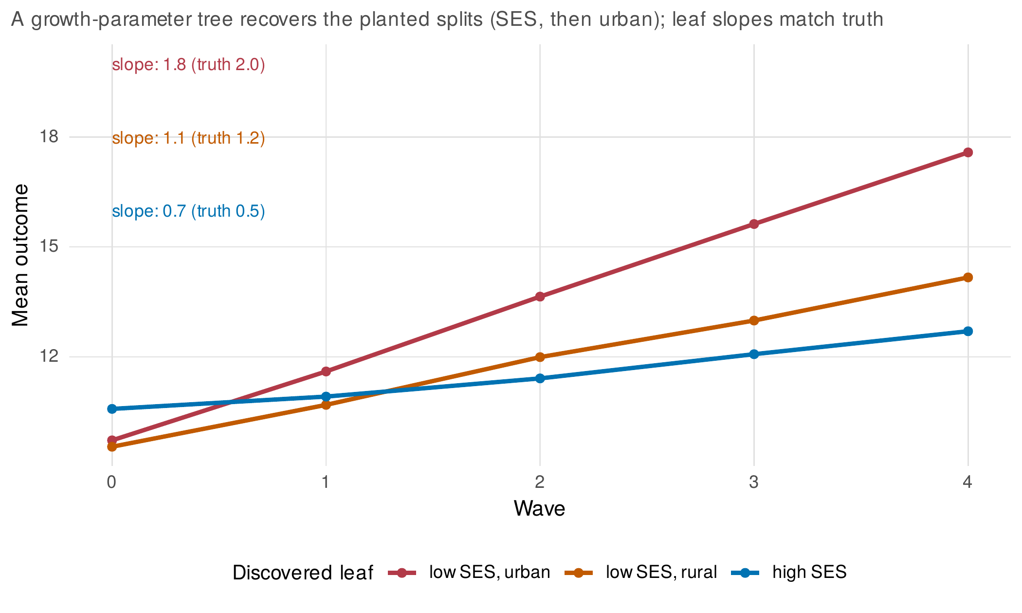
Note. Mean trajectories of the three subgroups a growth-parameter tree discovered in the growth_subgroups data. The tree split first on socioeconomic status and then on urban residence, the two true moderators, ignoring four noise covariates; the recovered leaf slopes on a held-out validation half (\(1.8\), \(1.1\), \(0.7\)) match the planted truth (\(2.0\), \(1.2\), \(0.5\)) up to the shrinkage of estimated person slopes. A discovered subgroup is a hypothesis to validate, not a finding certified by the search that produced it.
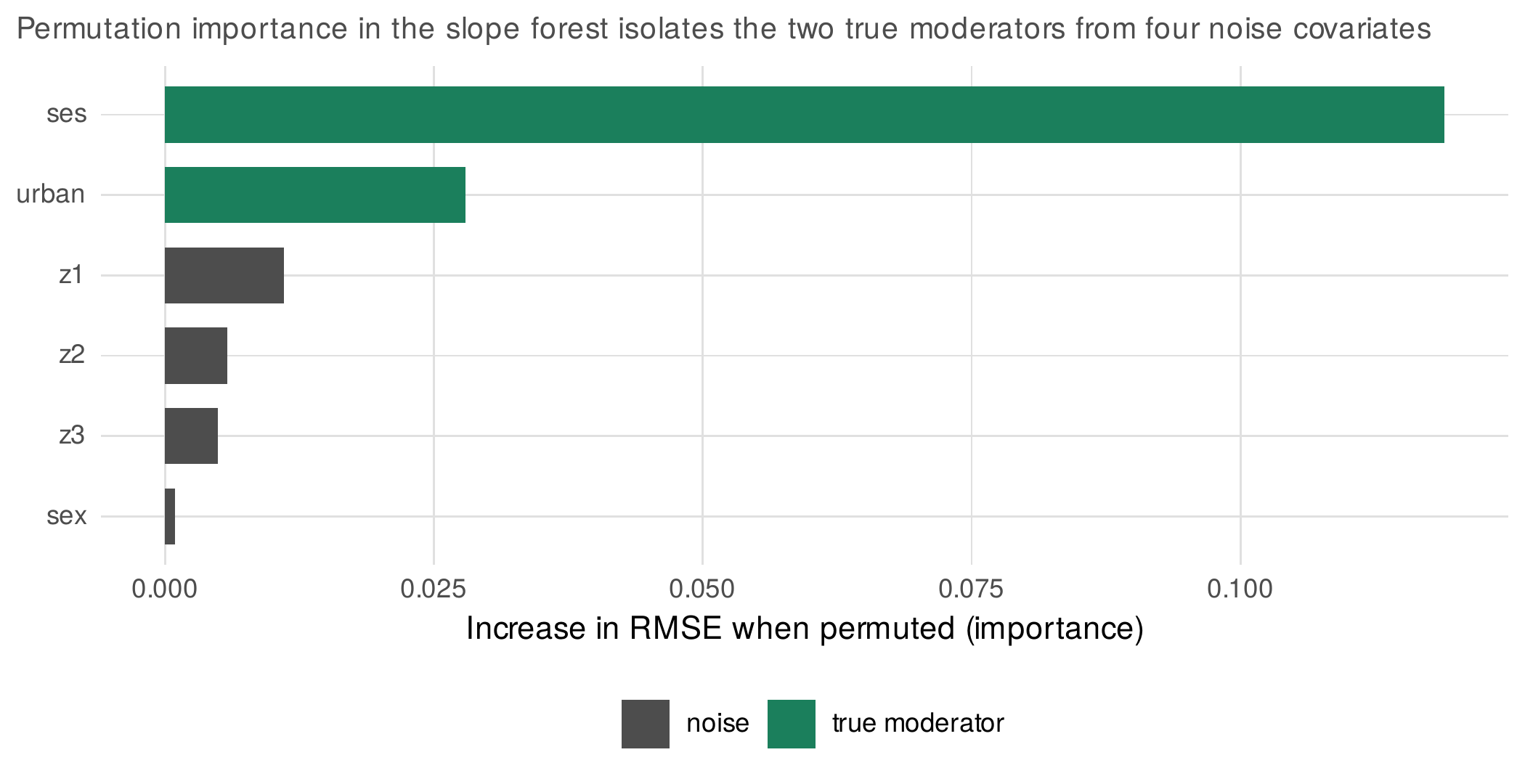
Note. Permutation importance, the increase in prediction error when a predictor is shuffled, from a forest predicting person growth slopes in the growth_subgroups data. Socioeconomic status and urban residence, the two true moderators, dominate; the four noise covariates sit near zero. Importance ranks predictive contribution and is read descriptively: it identifies features the model uses, not causes of the outcome.
Table 31.3. Tree and Forest Variants for Nested Longitudinal Data
| Method | What it partitions | Notes and maturity |
|---|---|---|
| Naive CART / RF | Fixed part, ignoring nesting | Importance biased toward cluster-correlated features; avoid for nested data |
| RE-EM tree | Fixed part, random effects retained | Alternates tree and random effects; mature (Sela & Simonoff) |
| GLMM tree | Fixed-effect subgroups, mixed model intact | Subgroup discovery; mature (glmertree) |
| Mixed-effects forest | Prediction with random effects | Longitudinal RF; ecosystem less settled (verify) |
| SEM tree / forest | Any latent-growth parameter | Heterogeneity in growth models; validate discoveries |
Note. The unifying principle is to let the algorithm search the fixed part while a mixed model absorbs the dependence, so that discovered subgroups reflect genuine fixed differences rather than cluster artifacts. Package maturity varies and moves; state the tool and its status in print, because readers are ill-served by citations to abandoned software.
31.4 Trajectory Clustering: The Algorithmic Rival
Trajectory clustering groups persons by the shape of their change over time, and it is the algorithmic counterpart to the model-based growth mixtures of Chapter 22. Where a growth mixture posits a probabilistic model, latent classes each with their own growth parameters, and estimates it by maximum likelihood with all the enumeration and fit machinery that entails, a clustering algorithm computes distances between trajectories and groups the near ones with no generative model at all. The k-means-for-longitudinal-data approach (Genolini & Falissard, 2010) treats each person’s sequence as a vector and applies k-means; distance-based variants replace Euclidean distance with a shape-aware distance such as dynamic time warping, which aligns sequences that share a shape but differ in timing before comparing them, appropriate when the timing of features is a nuisance to be removed rather than the signal itself, the same phase-versus-amplitude distinction Chapter 30 drew for registration.
The showdown pits the two philosophies against a known truth. The classes_sim data are generated from three latent growth classes, and Figure 31.6 compares a Gaussian mixture, trajectory k-means, and dynamic-time-warping clustering by how well each recovers the true class labels, measured by the adjusted Rand index. The model-based mixture wins, recovering the classes at an adjusted Rand index of \(0.90\), because its generative model matches the data-generating process; trajectory k-means follows at \(0.79\); and dynamic-time-warping clustering trails at \(0.71\), because its warping flexibility solves a phase-misalignment problem these data do not have and so discards useful amplitude information in the service of an alignment that was never needed. The ordering is not a universal ranking but a lesson about matching method to structure: when the generative model is known and correct, the model-based method is most efficient; when it is unknown or misspecified, the algorithmic methods are more robust; and dynamic time warping earns its keep only when timing misalignment is real. Table 31.4 states the trade-off, and it carries the doctrine of Chapter 22 verbatim: neither a mixture nor a clustering discovers real types, and a recovered grouping is a description to be validated externally, never a taxonomy certified by the algorithm that produced it.
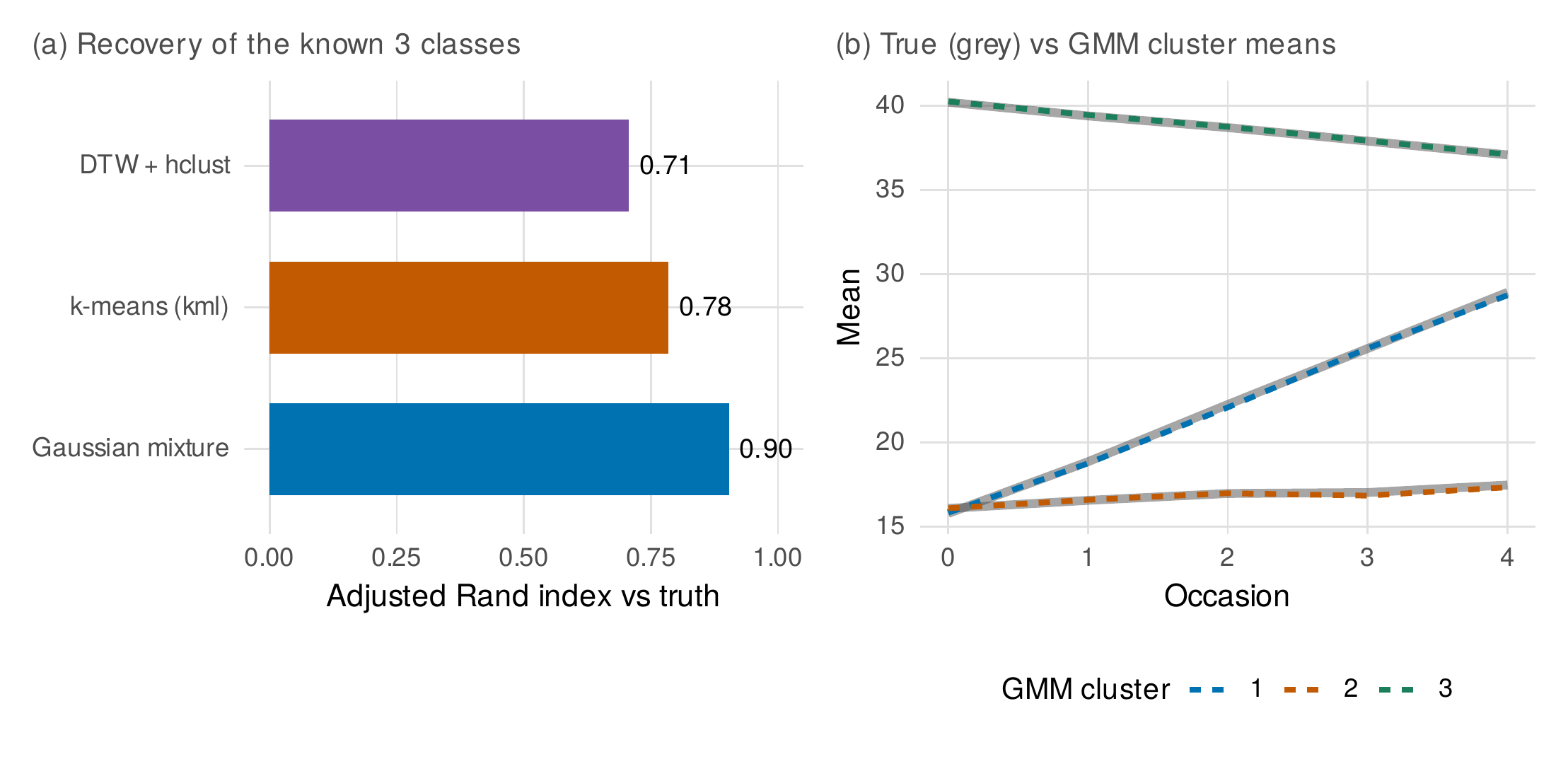
Note. Panel (a): recovery of the three true classes of the classes_sim data, by adjusted Rand index. The Gaussian mixture (\(0.90\)) wins because its generative model matches the data; trajectory k-means (\(0.79\)) follows; dynamic-time-warping clustering (\(0.71\)) trails because its warping addresses a timing misalignment these data do not contain. Panel (b): the true class-mean trajectories (grey) and the recovered mixture-cluster means (dashed) nearly coincide. The ranking is a lesson in matching method to structure, not a universal order.
Table 31.4. Model-Based Mixtures Versus Algorithmic Clustering
| Feature | Growth mixture (Ch. 22) | Trajectory clustering |
|---|---|---|
| Basis | Probabilistic generative model | Distance between trajectories |
| Output | Class probabilities, parameters, fit indices | Hard assignments |
| Strength | Efficient and inferential when correct | Robust when the model is unknown |
| Timing | Model-specified | DTW aligns phase if it is a nuisance |
| Shared caution | Neither discovers “real types”; a grouping is a description requiring external validation | |
Note. The choice is between a generative model that pays off when it matches the data and an algorithm that is robust when no model is trusted. Both produce groupings that look like discovered kinds and are not: the number of clusters is a modeling choice, and the substantive reality of a grouping must be argued from replication and external correlates, the doctrine shared with Chapter 22.
31.5 Regularization for Longitudinal Problems
Intensive designs create many-predictor problems: dozens of momentary items, their lags, their interactions, and their person-level aggregates can generate more candidate predictors than a classical regression can estimate. Regularization handles this by penalizing coefficient magnitude, shrinking small effects toward zero and, in the lasso, setting some exactly to zero, which performs selection and estimation at once. The penalty is the same shrinkage device that random effects apply, and it is the frequentist cousin of the Bayesian priors of Chapter 17, a connection worth holding onto because it demystifies regularization as disciplined shrinkage rather than a black art. Applied to screening next-occasion negative affect in the affect_ema data from a design matrix of momentary predictors, their lags, and all pairwise interactions, the lasso under person-grouped cross-validation selects a sparse model of seven predictors, retaining momentary stress, positive affect, and the lagged outcome along with a few interactions, and discarding the rest. Figure 31.7 shows the cross-validation path and the one-standard-error rule that chooses the sparse honest model.
Two longitudinal complications deserve care. First, when a predictor is decomposed into its within-person and between-person parts, as Chapter 7 recommended, the two components should be penalized as a pair or with awareness that penalizing them separately can distort the decomposition. Second, and more consequentially, the coefficients that survive selection do not carry the standard errors and p-values of an ordinary regression, because they were chosen by looking at the data, and post-selection inference that ignores this is invalid. The honest options are three: use the regularized model purely for prediction and report only out-of-sample skill; lock the selected model and refit it on a fresh sample where inference is valid; or split the data, selecting on one part and inferring on the other. The pragmatic doctrine is to keep selection and inference in separate compartments, and never to report a lasso coefficient with a naive confidence interval as though the selection had not happened.
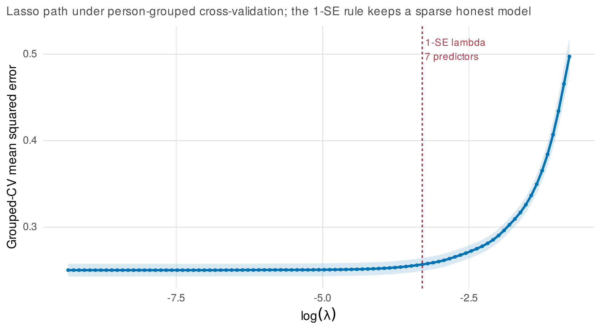
Note. The lasso cross-validation path for screening next-occasion negative affect in the affect_ema data, with folds grouped by person so that the selected model is honest for new persons. The error is flat across a wide range of penalties and rises as the penalty grows large; the one-standard-error rule (dashed) chooses a sparse model of seven predictors near the point where sparsity begins to cost accuracy. The selected coefficients are for prediction; inference on them requires a locked model or a fresh sample.
31.6 Idiographic Prediction and the Person-Specific Frontier
The predictive question can be turned inward, from generalizing across persons to forecasting a single person’s future, and here the pooling lesson of Chapter 25 returns in predictive clothing. Two strategies compete. A per-person model is fit to each individual’s own history and used to forecast their future, honoring idiographic variation completely; a pooled model borrows strength across persons, fitting one model to everyone and applying it to each. Which wins depends on how much history each person has, because a per-person model must estimate its parameters from that person’s data alone and is unreliable when the data are few. Figure 31.8 shows the crossover in the affect_ema data. With a short history of six occasions, the per-person model forecasts poorly, a root-mean-squared error of \(0.83\) against the pooled model’s \(0.47\), because six points cannot pin down an individual model; as the history lengthens the per-person error falls, overtaking the pooled model near twenty-four occasions, and with forty occasions the per-person model wins clearly. The lesson is the shrinkage lesson exactly: when data are sparse, pooling toward the population is the better bet, and only when a person has accumulated enough of their own data does an idiographic model earn its independence. The persistence baseline runs beneath both throughout, a reminder that yesterday’s value is a competitor neither model dominates by much.
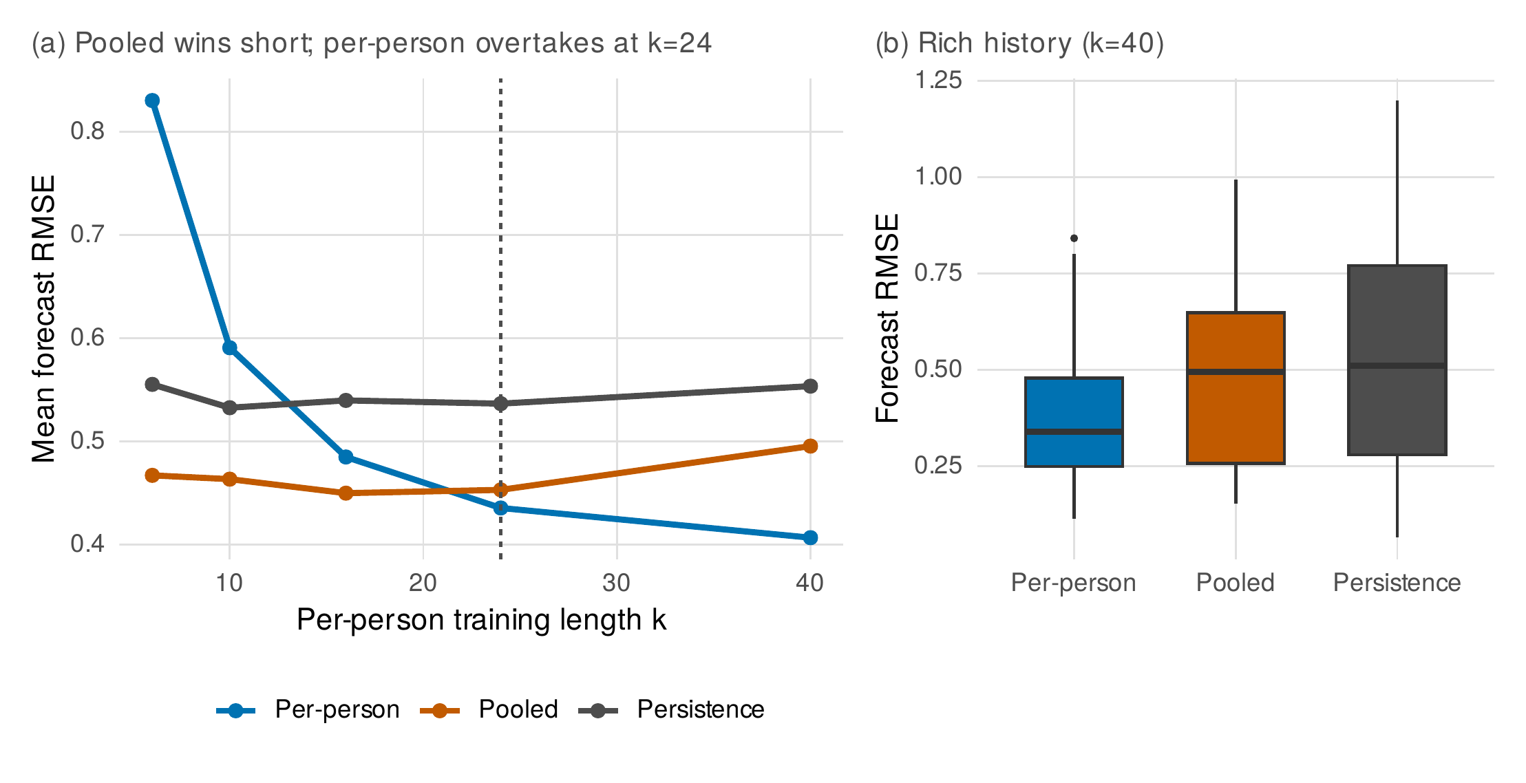
Note. Panel (a): mean within-person forecast error in the affect_ema data for a per-person model, a pooled model, and persistence, as the per-person training history lengthens. The per-person model is unreliable with a short history and improves as data accumulate, overtaking the pooled model near twenty-four occasions (dashed). Panel (b): with a rich forty-occasion history, the per-person error distribution is lowest. The crossover is the shrinkage lesson of Chapter 25 in predictive form: pool when data are sparse, individualize when they are rich.
Interpreting the models that result, whether pooled forests or per-person fits, requires tools that summarize a black box without overclaiming. Permutation importance, used above, ranks features by how much shuffling them degrades prediction, and it must be computed with the grouping respected, permuting within the resampling structure rather than across it. Partial-dependence and individual-conditional-expectation displays show how the predicted outcome moves as one feature varies with others held fixed or averaged, and Figure 31.9 shows the rising dependence of predicted negative affect on momentary stress, with individual curves revealing heterogeneity around the average. The essential discipline is that these displays are descriptive, not causal: the partial-dependence curve shows how the model’s prediction responds to a feature, which equals the causal effect of that feature only under assumptions the model does not verify and usually cannot. A rising partial-dependence curve for stress means the model predicts higher affect when stress is higher, not that reducing stress would lower affect, and the distance between those two readings is the distance between description and explanation the chapter opened by drawing. The forecasting displays, finally, must always be anchored to a baseline and reported with calibration as well as discrimination, Figure 31.10 placing every scheme’s error against the persistence line, and Table 31.5 listing the metrics and baselines a predictive report requires.
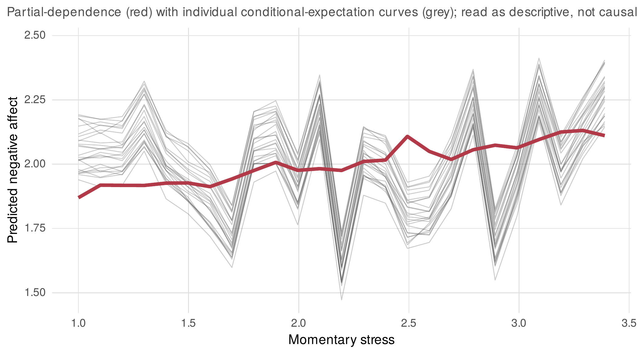
Note. The partial-dependence curve (red) shows how the forest’s predicted negative affect rises with momentary stress, averaged over the other features; the grey individual-conditional-expectation curves show that the dependence varies across observations. These displays describe the model’s behavior, not the world’s causal structure: the curve is the model’s response to a feature, which equals a causal effect only under untested assumptions. Read descriptively, they reveal what the model has learned to use.
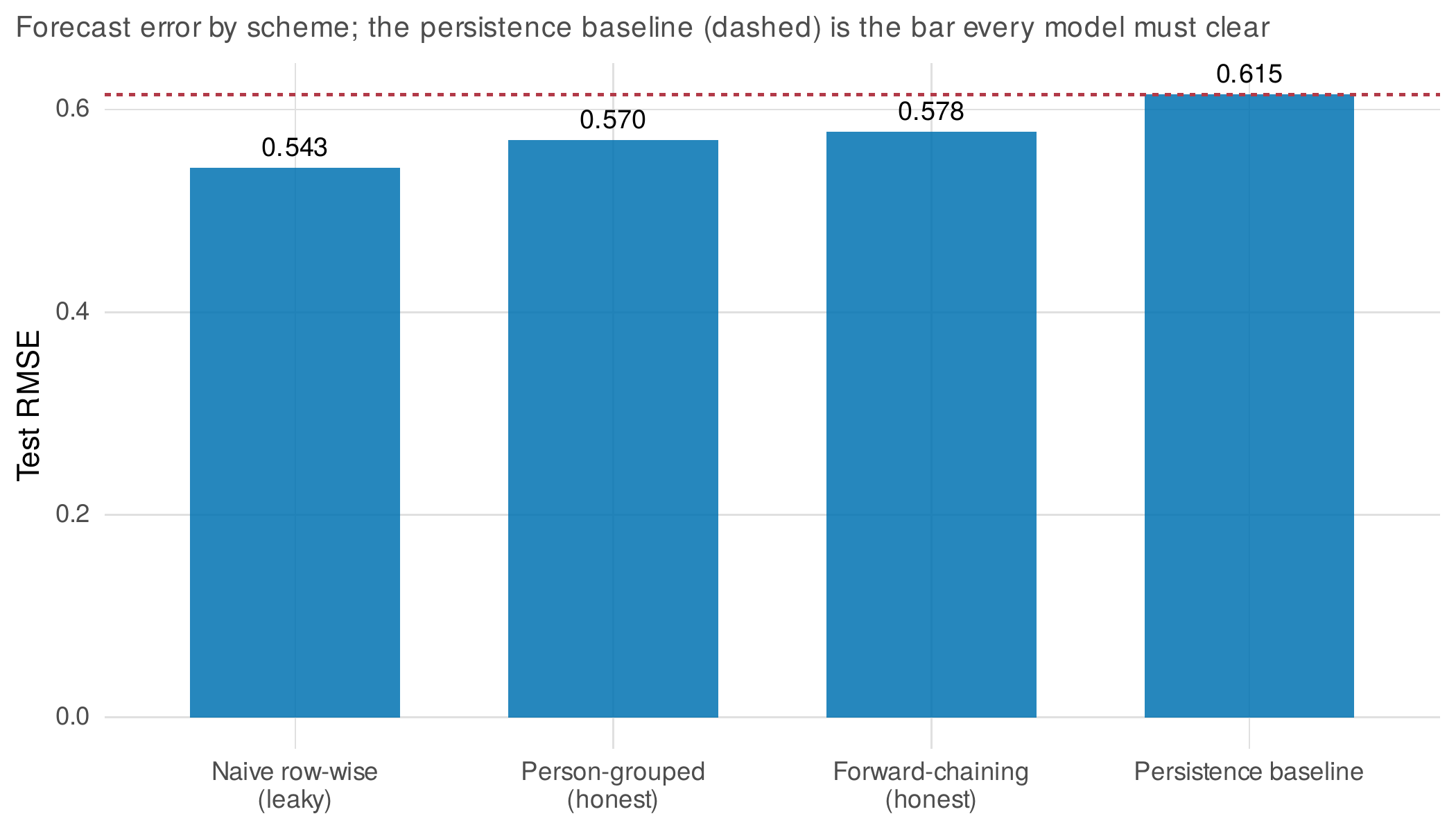
Note. Test root-mean-squared error for predicting momentary negative affect under each scheme, with the persistence baseline (dashed) marking the error of predicting the previous value. The naive scheme’s low error is the leakage of Figure 31.2 in error-metric form; the honest schemes sit just below persistence. A predictive claim is only as strong as its margin over the simplest baseline, which for longitudinal outcomes is almost always persistence.
Table 31.5. Performance Metrics and Mandatory Baselines
| Outcome type | Metrics (discrimination + calibration) | Mandatory baseline |
|---|---|---|
| Continuous | RMSE, \(R^2\); calibration of predicted vs observed | Persistence (previous value); person mean |
| Binary event | AUC, Brier score; calibration curve | Base rate; last observation |
| Time-to-event | Concordance; calibration at horizons | Kaplan-Meier (Ch. 29) |
Note. Discrimination (ordering cases) and calibration (matching predicted to observed magnitudes) are distinct; a model can discriminate well and be miscalibrated, so both are reported (Steyerberg, 2019). Every predictive claim is stated as a margin over a baseline; for longitudinal outcomes the persistence baseline, predicting no change, is the one a model must beat to have shown anything.
31.7 Reporting and Preregistration
A predictive study earns trust by reporting the decisions that determine whether its accuracy is real, and the reporting standards developed for clinical prediction models transfer directly (Collins et al., 2015). The performance must be reported with uncertainty, from repeated resampling, and against the mandatory baseline, so a reader can see both how accurate the model is and how much it improves on doing nothing. The resampling scheme must be named and justified, and the leakage audit made explicit: how folds respected persons and time, where preprocessing sat relative to the split, and how tuning was nested. The distinction between what was fixed in advance and what the data chose must be preserved, because it is what allows a machine-learning analysis to be preregistered at all. A preregistration can fix the resampling scheme, the metrics, the baselines, the tuning grid, and the feature set, leaving only the fitted model to the data, and an analysis conducted this way occupies the honest exploratory lane the book returns to in Chapter 36: exploratory in that the model is discovered, confirmatory in that the evaluation was specified before the model was seen. Table 31.6 is the checklist, the software box states the package-maturity audit the chapter has promised, and the practice box addresses the compute and reproducibility realities of running these analyses at scale.
Table 31.6. Reporting Checklist for Longitudinal Machine Learning
| Element | What to report |
|---|---|
| Estimand and task | Prediction, description, or explanation; new-person vs within-person |
| Resampling | Scheme (grouped / forward-chaining), why, and the leakage audit |
| Baselines | Persistence and other baselines, with the model’s margin over them |
| Performance | Discrimination and calibration, with uncertainty from repeated CV |
| Tuning | Hyperparameter grid and how it was nested inside training folds |
| Fixed vs chosen | What was preregistered vs what the data determined |
| Software | Packages and versions, with maturity status stated candidly |
Note. The reporting is organized around the decisions a reader cannot otherwise verify: how leakage was avoided and how much the model beats a baseline. An analysis that fixes the scheme, metrics, baselines, and grid in advance and lets the data choose only the model is both exploratory and honest, the lane Chapter 36 formalizes.
Software Note • A package-maturity audit
The tools for longitudinal machine learning vary widely in maturity, and candor about this serves readers who will otherwise cite abandonware. For mixed-effects trees, glmertree and partykit are mature and maintained; RE-EM trees have a reference implementation of longer standing. For longitudinal forests, LongituRF implements the methods but is less battle-tested than cross-sectional forest packages. For trajectory clustering, kml is established and dtwclust is the standard for distance-based clustering; latrend aims to unify the interfaces but should be checked for current status. For regularized structural models, regsem implements the methods of Jacobucci et al. (2016). For grouped resampling, rsample within tidymodels provides the idioms, though its interface evolves. Because none of these are in the base toolkit and several were unavailable in the environment that produced this chapter, the analyses here hand-build the core logic, the forest, the dynamic-time-warping distance, the mixture, and every resampling scheme, on rpart, glmnet, and base R, which is both a reproducibility safeguard and a demonstration that the ideas are simpler than their packages.
In Practice • Compute, seeds, and reproducibility
Cross-validated machine learning is stochastic in its splits, its bootstrap samples, and its feature subsets, so reproducibility requires setting and recording seeds at every stochastic step, and honest uncertainty requires repeating the whole resampling several times rather than trusting a single split. Compute grows with the product of folds, repeats, trees, and tuning-grid points, and the person-grouped and forward-chaining schemes add bookkeeping that a naive loop does not; budgeting this before a large run, and parallelizing across folds with per-worker seeds for reproducibility, prevents both wasted time and irreproducible results. The discipline is the lab standard of the book: seeds set, conditions gridded, results archived with the code that produced them, so that a number in a table can be regenerated exactly.
Chapter Summary
Machine learning serves longitudinal research when it is matched to the research goal and disciplined against the leakage that dependent data invite. Breiman’s two cultures, explanation through an interpretable model and prediction through any validated function, are goals to choose between rather than rivals to adjudicate, and the estimand-first rule assigns each question its method and its standard of evidence, guarding against the category error of reading prediction as explanation. The load-bearing discipline is honest evaluation: naive row-wise cross-validation of repeated measures leaks, testing a model partly on persons it has seen, and on the affect_ema data it overstates predictive \(R^2\) by seventeen percent relative to person-grouped cross-validation, which holds out whole persons to estimate new-person error, and forward-chaining, which trains on the past to estimate forecasting error; the persistence baseline shows the honest model beats yesterday’s value only modestly. Preprocessing and tuning belong inside the training folds, and the leakage audit, not the accuracy, is what a reader should demand. Trees and forests for nested data keep the random-effects structure while searching the fixed part: a growth-parameter tree recovers planted subgroups in the growth_subgroups data, splitting on the two true moderators and ignoring four noise covariates, with validated leaf slopes matching truth, and permutation importance separates signal from noise while remaining descriptive rather than causal. Trajectory clustering is the algorithmic rival to Chapter 22’s mixtures, and against a known three-class truth the model-based mixture wins (adjusted Rand index \(0.90\)) because its model matches the data, k-means follows, and dynamic-time-warping clustering trails because its warping solves a timing problem the data do not have; neither method discovers real types, and a grouping is a description to validate. Regularization handles many-predictor problems as disciplined shrinkage, selecting a sparse honest model under grouped cross-validation, but its selected coefficients carry no ordinary inference and must be locked or split before p-values are attached. Idiographic forecasting replays the shrinkage lesson: the pooled model beats the per-person model for short histories and loses to it once a person accumulates enough data, crossing over near twenty-four occasions, and every forecast is judged against persistence. Partial-dependence and importance displays interpret black boxes descriptively, never causally, and the reporting standard fixes the scheme, baselines, metrics, and grid in advance so that a discovered model is evaluated by a specified rule, exploratory in its model and confirmatory in its evaluation.
Brandmaier, A. M., Prindle, J. J., McArdle, J. J., & Lindenberger, U. (2016). Theory-guided exploration with structural equation model forests. Psychological Methods, 21(4), 566–582. https://doi.org/10.1037/met0000090
Brandmaier, A. M., von Oertzen, T., McArdle, J. J., & Lindenberger, U. (2013). Structural equation model trees. Psychological Methods, 18(1), 71–86. https://doi.org/10.1037/a0030001
Breiman, L. (2001). Statistical modeling: The two cultures. Statistical Science, 16(3), 199–231. https://doi.org/10.1214/ss/1009213726
Capitaine, L., Genuer, R., & Thiébaut, R. (2021). Random forests for high-dimensional longitudinal data. Statistical Methods in Medical Research, 30(1), 166–184. https://doi.org/10.1177/0962280220946080
Collins, G. S., Reitsma, J. B., Altman, D. G., & Moons, K. G. M. (2015). Transparent reporting of a multivariable prediction model for individual prognosis or diagnosis (TRIPOD): The TRIPOD statement. BMJ, 350, Article g7594. https://doi.org/10.1136/bmj.g7594
Fokkema, M., Smits, N., Zeileis, A., Hothorn, T., & Kelderman, H. (2018). Detecting treatment-subgroup interactions in clustered data with generalized linear mixed-effects model trees. Behavior Research Methods, 50(5), 2016–2034. https://doi.org/10.3758/s13428-017-0971-x
Genolini, C., & Falissard, B. (2010). KmL: K-means for longitudinal data. Computational Statistics, 25(2), 317–328. https://doi.org/10.1007/s00180-009-0178-4
Hajjem, A., Bellavance, F., & Larocque, D. (2014). Mixed-effects random forest for clustered data. Journal of Statistical Computation and Simulation, 84(6), 1313–1328. https://doi.org/10.1080/00949655.2012.741599
Hastie, T., Tibshirani, R., & Friedman, J. (2009). The elements of statistical learning: Data mining, inference, and prediction (2nd ed.). Springer. https://doi.org/10.1007/978-0-387-84858-7
Jacobson, N. C., & Nemesure, M. D. (2021). Using artificial intelligence to predict change in depression and anxiety symptoms in a digital intervention: Evidence from a transdiagnostic randomized controlled trial. Psychiatry Research, 295, Article 113618. https://doi.org/10.1016/j.psychres.2020.113618
Jacobucci, R., Grimm, K. J., & McArdle, J. J. (2016). Regularized structural equation modeling. Structural Equation Modeling: A Multidisciplinary Journal, 23(4), 555–566. https://doi.org/10.1080/10705511.2016.1154793
James, G., Witten, D., Hastie, T., & Tibshirani, R. (2021). An introduction to statistical learning with applications in R (2nd ed.). Springer. https://doi.org/10.1007/978-1-0716-1418-1
Molnar, C. (2022). Interpretable machine learning: A guide for making black box models explainable (2nd ed.). Independently published. https://christophm.github.io/interpretable-ml-book/
Roberts, D. R., Bahn, V., Ciuti, S., Boyce, M. S., Elith, J., Guillera-Arroita, G., Hauenstein, S., Lahoz-Monfort, J. J., Schröder, B., Thuiller, W., Warton, D. I., Wintle, B. A., Hartig, F., & Dormann, C. F. (2017). Cross-validation strategies for data with temporal, spatial, hierarchical, or phylogenetic structure. Ecography, 40(8), 913–929. https://doi.org/10.1111/ecog.02881
Sela, R. J., & Simonoff, J. S. (2012). RE-EM trees: A data mining approach for longitudinal and clustered data. Machine Learning, 86(2), 169–207. https://doi.org/10.1007/s10994-011-5258-3
Sardá-Espinosa, A. (2019). Time-series clustering in R using the dtwclust package. The R Journal, 11(1), 22–43. https://doi.org/10.32614/RJ-2019-023
Shmueli, G. (2010). To explain or to predict? Statistical Science, 25(3), 289–310. https://doi.org/10.1214/10-STS330
Steyerberg, E. W. (2019). Clinical prediction models: A practical approach to development, validation, and updating (2nd ed.). Springer. https://doi.org/10.1007/978-3-030-16399-0
Varma, S., & Simon, R. (2006). Bias in error estimation when using cross-validation for model selection. BMC Bioinformatics, 7, Article 91. https://doi.org/10.1186/1471-2105-7-91
Yarkoni, T., & Westfall, J. (2017). Choosing prediction over explanation in psychology: Lessons from machine learning. Perspectives on Psychological Science, 12(6), 1100–1122. https://doi.org/10.1177/1745691617693393