Chapter 32
Nonlinear Dynamics: Regime Switching, Differential Equations, and Early Warning Signals
The models of the preceding chapters, for all their sophistication, share an ontology: change is a smooth, gradual, and reversible flow around a single equilibrium, disturbed by noise but tending always back to one central tendency. Many of the phenomena psychologists most want to understand violate that ontology. Relapse is a switch, not a drift; mood can cycle rather than settle; addiction shows hysteresis, so that the same stressor produces recovery or collapse depending on the history that precedes it; and a depressive episode can arrive as a sudden transition between alternative stable states rather than a slow slide. This chapter develops the machinery for genuinely nonlinear hypotheses, and it does so with the book’s most careful attention to the gap between what the machinery promises and what the evidence supports, because this is the frontier where that gap is widest. Three formalisms organize the material. Regime-switching models treat the system as occupying one of a few discrete states with its own dynamics, and a hidden Markov model or a Markov-switching autoregression estimates the states and the transitions between them. Differential-equation models formalize regulation as a restoring force, and the damped linear oscillator gives frequency and damping a psychological reading as the tempo and thoroughness of a return to equilibrium. Critical-transition theory treats a sudden shift as the loss of stability of one state, and it predicts early-warning signals, a rising autocorrelation and variance as the system slows near the tipping point, that have been proposed as a basis for anticipating clinical transitions. Each formalism is powerful and each is easy to oversell, so the chapter pairs every method with the discipline that keeps it honest: the enumeration caution of Chapter 22 for regimes, the embedding-sensitivity candor that oscillator estimation demands, and the surrogate inference and single-case sobriety that early-warning signals require. The honesty is not a hedge appended to the content; on this frontier it is the content.
Learning Objectives
After working through this chapter, you should be able to: (1) recognize when a linear, single-equilibrium model is the wrong ontology and formulate a nonlinear alternative as a substantive hypothesis; (2) fit and interpret regime-switching models, hidden Markov models and Markov-switching autoregressions, and adjudicate the number of regimes with the enumeration discipline of Chapter 22; (3) understand differential-equation modeling of regulation, estimate a damped linear oscillator by generalized local linear approximation, and confront its embedding sensitivity honestly; (4) explain critical slowing down and compute early-warning indicators with proper surrogate-based inference; (5) evaluate the early-warning-signal evidence in psychopathology candidly; (6) use recurrence quantification as a descriptive lens; and (7) match each nonlinear method to a realistic data budget and claim ceiling.
32.1 When Linearity Is the Wrong Theory
Nonlinearity is a substantive claim, not a decorative one, and it must be defended substantively. The default of the book has been the linear, single-equilibrium model, and that default is often right, both because many processes are approximately linear near their equilibrium and because a linear approximation is principled where a nonlinear elaboration is merely fashionable. The case for a nonlinear model is made when the phenomenon exhibits a signature that a linear model cannot produce, and Figure 32.1 collects four such signatures. A regime switch shows an abrupt change in level or dynamics that a smooth trend misrepresents. A sustained cycle shows periodicity that a mean-reverting model treats as noise. A hysteresis loop shows that the state depends on the history of a forcing variable, so that the same input yields different outputs on the way up and the way down, which no static input-output function captures. And a bimodal marginal distribution shows two preferred states where a linear-Gaussian model assumes one. These signatures are the empirical warrant for going nonlinear, and their absence is a warrant for staying linear.
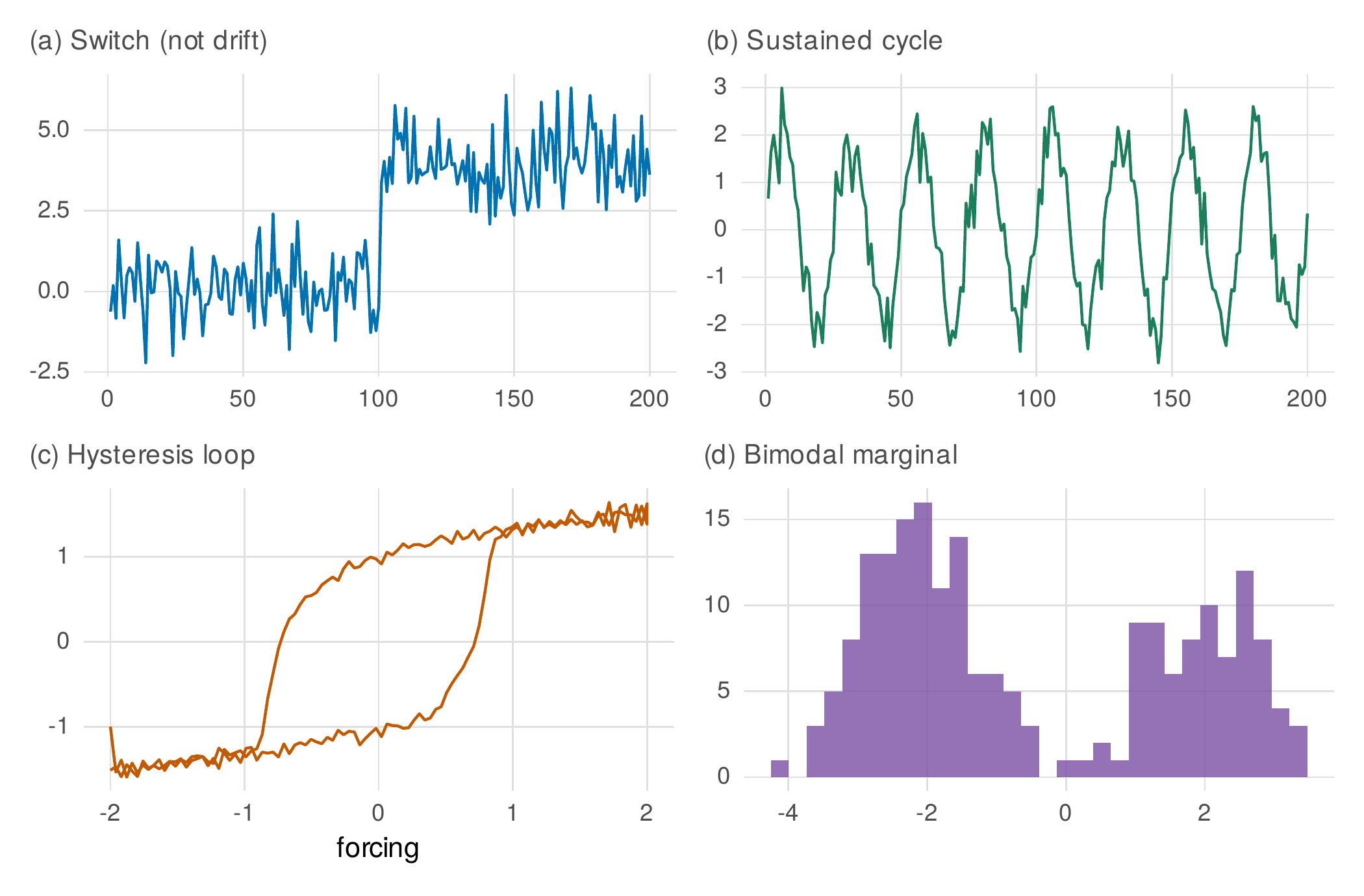
Note. (a) A regime switch: an abrupt change in level that a smooth trend misrepresents. (b) A sustained cycle: periodicity a mean-reverting model treats as noise. (c) A hysteresis loop: the state depends on the history of the forcing, so the up and down paths differ, which no static function captures. (d) A bimodal marginal: two preferred states where a linear-Gaussian model assumes one. Each signature is a substantive warrant for a nonlinear model; their absence is a warrant for staying linear.
Three formalisms handle these phenomena, and Figure 32.2 maps them. Discrete regimes, in which the system occupies one of a few states each with its own dynamics, are the province of the regime-switching models of Section 32.2. Continuous nonlinear flows, in which a restoring force pulls the system back toward equilibrium along a curved path, are the province of the differential-equation models of Section 32.3. Transitions between alternative stable states, in which a slowly changing condition carries the system past a tipping point, are the province of the critical-transition theory of Section 32.4. The linear tools of the earlier chapters sit inside this larger picture as the local, near-equilibrium approximations that suffice when none of the nonlinear signatures is present. Table 32.1 is the orientation, mapping each phenomenon to its formalism and the chapter’s tool.
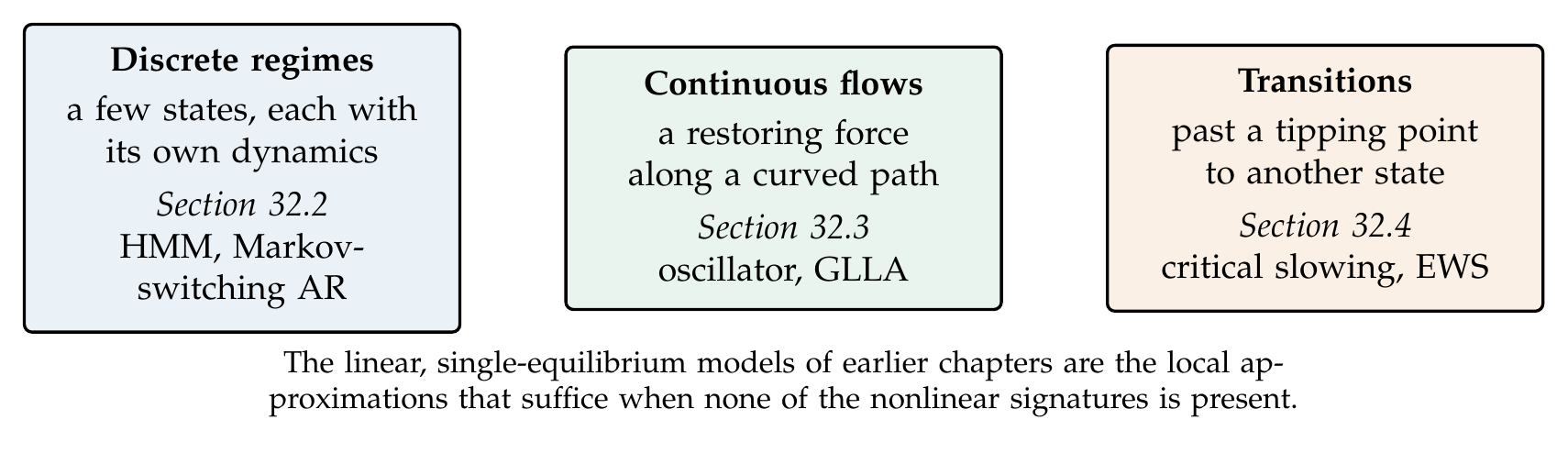
Note. Nonlinear phenomena fall into three families, each with its own machinery: discrete regimes handled by state-switching models, continuous nonlinear flows handled by differential equations, and transitions between alternative stable states handled by critical-transition theory. Recurrence quantification (Section 32.5) is a descriptive lens applicable across all three. The chapter’s linear predecessors are the near-equilibrium special case.
Table 32.1. Nonlinear Phenomena, Formalisms, and Tools
| Phenomenon | Formalism | Tool (section) |
|---|---|---|
| Sudden switch in state | Discrete regimes | HMM, Markov-switching AR (32.2) |
| Sustained oscillation | Continuous flow | Damped oscillator, GLLA (32.3) |
| Hysteresis, tipping | Alternative stable states | Critical slowing, EWS (32.4) |
| Recurrence structure | (descriptive) | Recurrence quantification (32.5) |
| Smooth reversible change | Single equilibrium | Linear models (earlier chapters) |
Note. The formalism follows from the phenomenon, and the phenomenon must be demonstrated, not assumed. A single reported hazard ratio or growth slope presumes the last row; the signatures of Figure 32.1 are what license the others. Nonlinearity is a hypothesis with its own burden of proof.
32.2 Regime-Switching Models
A regime-switching model supposes that the system occupies one of a small number of hidden states, each with its own distribution or dynamics, and that it moves among them according to a Markov transition structure. The simplest version is the hidden Markov model, in which each state has its own emission distribution and the observations are conditionally independent given the state; it is the measurement-simple kin of the latent transition models of Chapter 22, and it is estimated by the same forward-backward expectation-maximization logic. Applied to the n1_mood series, a single person’s daily valence over two hundred days with a planted progression from a stable regime through a transition to a depressed one, a three-state hidden Markov model recovers the structure. Its Bayesian information criterion prefers three states over two (\(1451\) versus \(1504\)), it decodes the planted regimes with eighty-five percent accuracy, and its state means, \(28.7\), \(53.6\), and \(67.4\), track the planted regime means; the depressed state also carries the largest emission standard deviation, \(12.9\) against \(4.3\) in the stable state, the rising variability that Section 32.4 will read as a warning sign. Figure 32.3 shows the decoding with its posterior state probabilities, and the display convention matters: the deliverable is not a hard coloring that asserts each day’s state with false certainty but the posterior probability of each state at each time, which shows confidently classified stretches and genuinely ambiguous transitions alike.
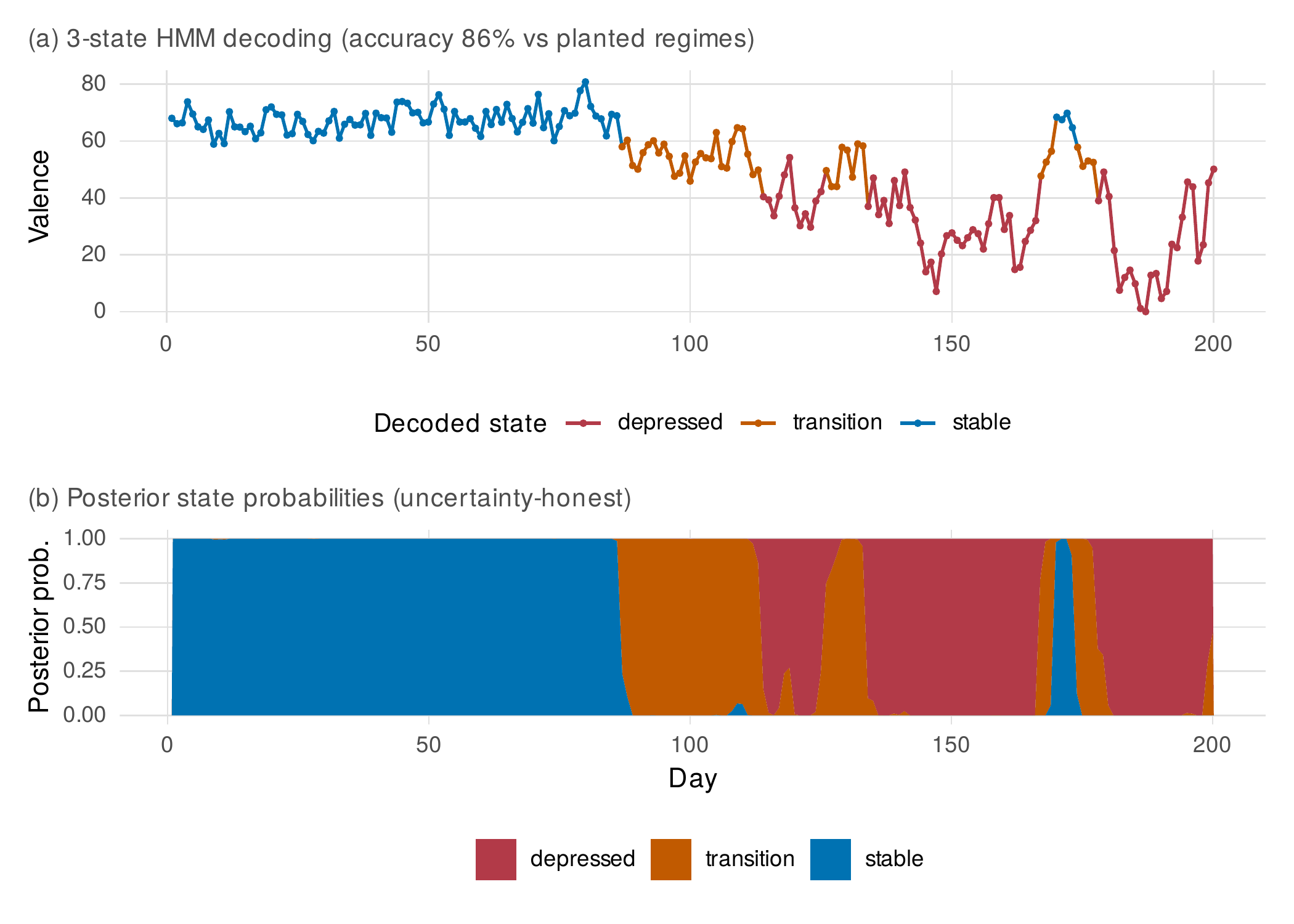
Note. Panel (a): the n1_mood valence series colored by the most probable decoded state of a three-state hidden Markov model, which recovers the planted stable, transition, and depressed regimes at eighty-five percent accuracy. Panel (b): the posterior probability of each state at each day, the uncertainty-honest deliverable. Confident stretches show a single state near probability one; genuine transitions show mixed probabilities. Reporting hard state labels instead would assert a certainty the data do not support.
The richer version lets the dynamics, not merely the mean, differ across regimes. A Markov-switching autoregression gives each regime its own autoregressive persistence and innovation variance, formalizing the clinically resonant idea that a person’s mood is not merely lower in a depressed regime but differently regulated, more inertial and more volatile. Decoding the n1_mood regimes and estimating the within-regime dynamics bears this out: the depressed regime shows an autoregressive persistence of \(0.75\) and an innovation standard deviation of \(8.97\), against \(0.29\) and \(4.14\) in the stable regime, a dysregulation visible in the dynamics themselves and not just the level. Figure 32.4 displays the contrast. The joint estimator that fits the regimes and their regime-specific dynamics simultaneously, implemented in the dynr package, is the gold standard and shares the state-space machinery of Chapter 26; the two-step decode-then-estimate used here is its transparent approximation. Table 32.2 lays out the specification anatomy of a regime-switching state-space model, including the covariate-dependent transition probabilities, a stressor raising the probability of switching into the dysregulated regime, that make the framework a genuine model of what precipitates a transition rather than merely a description that one occurred.
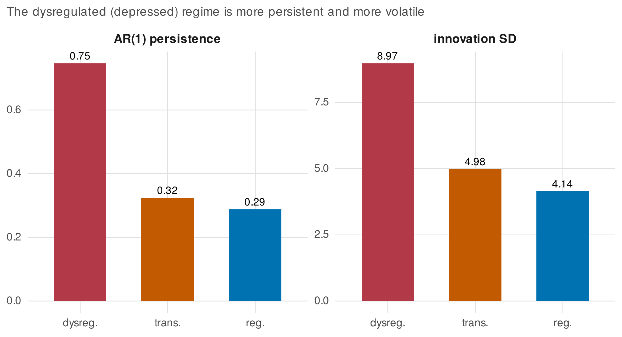
Note. Autoregressive persistence and innovation standard deviation estimated within each decoded regime of the n1_mood series. The depressed (dysregulated) regime shows both higher persistence (\(0.75\) versus \(0.29\)) and larger innovations (\(8.97\) versus \(4.14\)) than the stable (regulated) regime, so the regimes differ in their dynamics, not only their mean level. This is the clinically substantive content a mean-only description misses.
Table 32.2. Anatomy of a Regime-Switching State-Space Specification
| Component | What it specifies | Psychological reading |
|---|---|---|
| Regime dynamics | AR/VAR coefficients per regime | Regulated vs dysregulated dynamics |
| Innovation variance | Noise magnitude per regime | Volatility of the state |
| Initial probabilities | Regime at the first occasion | Starting state |
| Transition matrix | Probabilities of staying/switching | Persistence of regimes |
| Covariate transitions | Predictors of switch probability | What precipitates a transition |
Note. The transition structure is what distinguishes a regime-switching model from a mixture: it models the temporal order of states and what drives movement among them. Covariate-dependent transitions turn the model from a description of when regimes occurred into a hypothesis about their precipitants. Estimation shares the starting-value and label-switching cautions of Chapters 22 and 26.
The enumeration discipline of Chapter 22 transfers intact and is the section’s epistemic keystone. A two-state model will fit many series that have no genuine regimes at all, because heavy-tailed or heteroscedastic noise from a single regime mimics the appearance of switching. Figure 32.5 shows the trap: a genuine two-regime series and a single-regime series with heavy-tailed noise are both fit by a two-state model, and the fit alone cannot distinguish them. The safeguards are the ones Chapter 22 named: the posterior regime probabilities reported honestly rather than hardened into labels, the coherence of the decoded regimes with external covariates, and replication. A recovered regime, like a recovered latent class, is a hypothesis about structure, validated by what it predicts and whether it recurs, never a discovery certified by the model that found it.
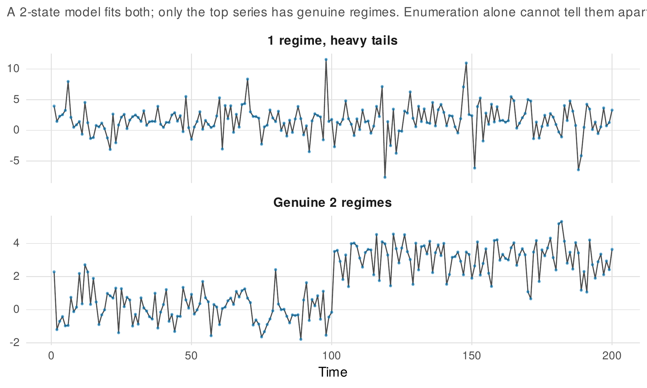
Note. Two series a two-state model fits equally well: a genuine two-regime process (top) and a single-regime process with heavy-tailed noise (bottom). Model fit alone cannot tell them apart, because heavy tails from one regime mimic switching between two. The safeguards are external: coherence of the decoded regimes with covariates, honest posterior uncertainty, and replication, the enumeration discipline of Chapter 22.
32.3 Differential Equations and the Oscillator
Where regulation is the theory, differential equations are its natural language, because a restoring force is a statement about a derivative: the rate of change of a state depends on how far the state is from its set point. The canonical formalization is the damped linear oscillator, \(\ddot{x} = \eta\,x + \zeta\,\dot{x}\), in which the acceleration of the state depends on its displacement through a frequency parameter \(\eta\) and on its velocity through a damping parameter \(\zeta\). The psychological reading is the emotion-as-thermostat metaphor made quantitative (Chow et al., 2005): a negative \(\eta\) produces oscillation, the overshoot and return of a system pulled back toward its set point, and a negative \(\zeta\) damps that oscillation, so that the amplitude decays and the system settles. Frequency indexes how fast the person cycles around their equilibrium, damping how thoroughly each excursion is regulated away, and individual differences in these parameters are the substantive payoff: a poorly damped emotional system oscillates for longer after a perturbation, a plausible operationalization of emotional dysregulation. Figure 32.6 shows the parameter regimes and their trajectories.
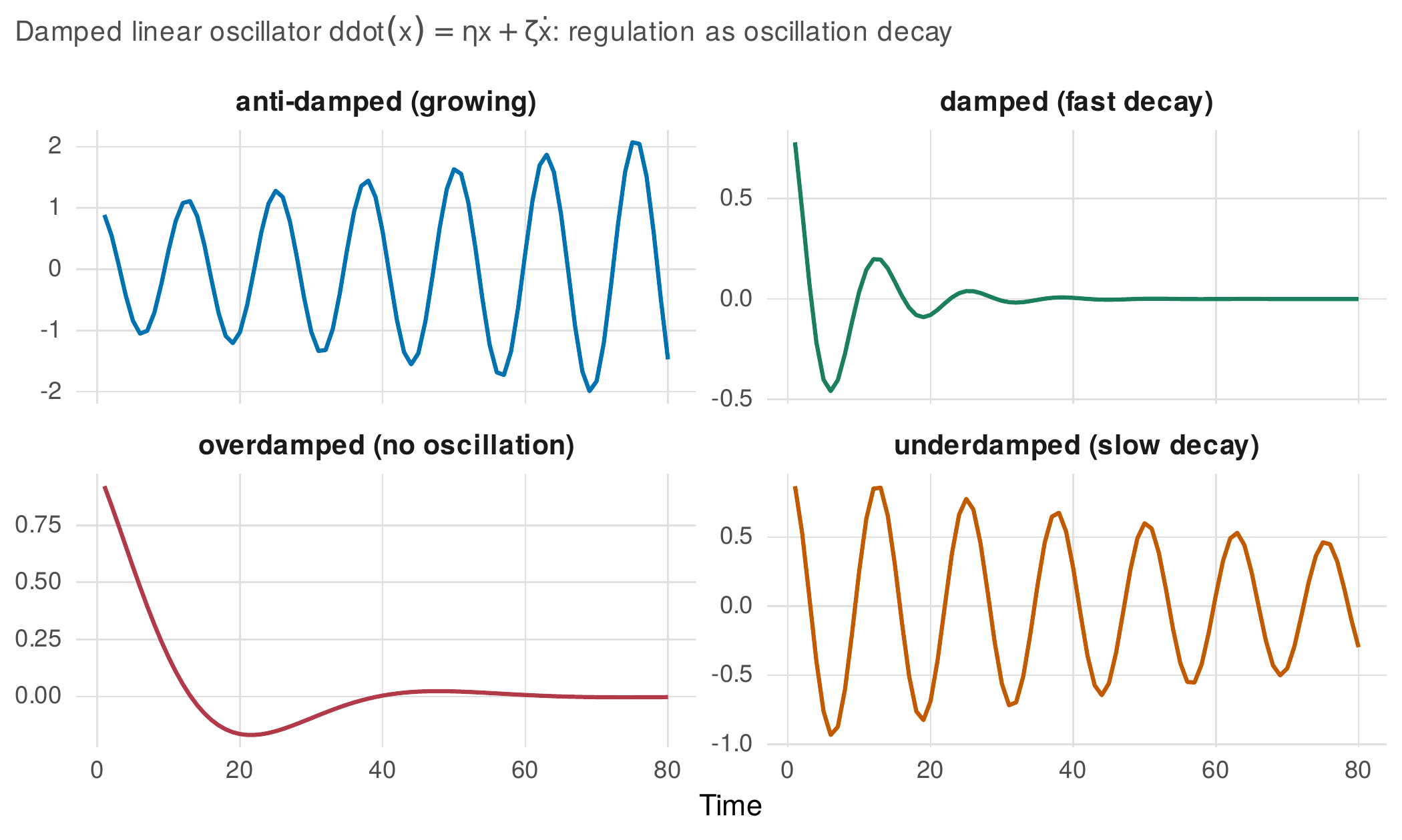
Note. Trajectories of the damped linear oscillator \(\ddot{x}=\eta x + \zeta\dot{x}\) for four parameter regimes. Underdamped with slow decay: sustained visible oscillation. Damped: oscillation that settles quickly. Anti-damped (\(\zeta>0\)): growing oscillation, a runaway system. Overdamped (\(\eta\) near zero): return to equilibrium with no oscillation at all, indistinguishable from simple mean reversion. Regulation is the decay of oscillation; dysregulation is its persistence or growth.
Estimating the oscillator requires estimating derivatives from discrete, noisy data, and the generalized local linear approximation (GLLA) does so by embedding the series, forming overlapping windows of \(D\) consecutive observations, and applying a fixed linear operator that fits a local second-order polynomial to recover the level, velocity, and acceleration at each point (Boker & Nesselroade, 2002). Regressing the estimated acceleration on the estimated level and velocity yields \(\eta\) and \(\zeta\). On a known damped oscillator (\(\eta = -0.25\), \(\zeta = -0.06\), period \(12.6\)), GLLA recovers the parameters well at an embedding dimension of four (\(\hat\eta = -0.26\), \(\hat\zeta = -0.05\), period \(12.3\)). But the estimates depend on the embedding dimension, and this dependence is the method’s central fragility, taught rather than hidden. Figure 32.7 is the candor set piece: as the embedding dimension varies from three to nine, the frequency estimate drifts from \(-0.32\) to \(-0.19\), bracketing but not pinning the truth. An oscillator analysis that reports a single \((\eta, \zeta)\) without showing its sensitivity to the embedding choice is concealing the most important thing about it, and the honest report is the sensitivity curve, not the point estimate.
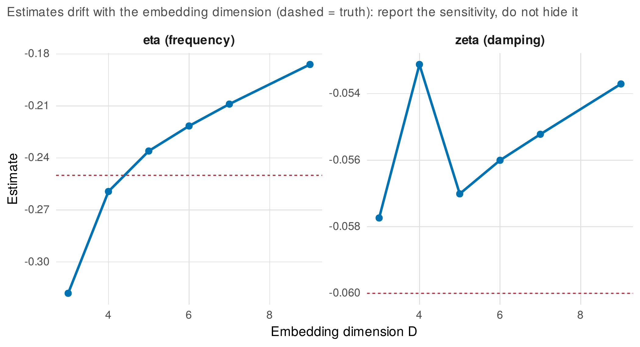
Note. Generalized-local-linear-approximation estimates of the oscillator frequency (\(\eta\)) and damping (\(\zeta\)) as the embedding dimension varies, for a series with known parameters (dashed). The frequency estimate drifts systematically with the embedding choice, bracketing the truth rather than pinning it; the damping estimate is more stable but not fixed. The embedding dimension is a researcher degree of freedom, and reporting the sensitivity across it, not a single point estimate, is the honest practice.
The fragility deepens on real data, and the payoff must be stated with a corresponding caution. Fitting the oscillator to each person’s positive-affect series in the affect_ema data, every person’s estimate has a negative frequency and satisfies the underdamped condition, which would seem to say that everyone oscillates. They do not. A negative frequency estimate means only that the series is mean-reverting, and a noisy mean-reverting process embedded and differentiated looks locally oscillatory to GLLA whether or not it contains any genuine cycle. The oscillator model, in other words, fits almost everything, which is exactly why an oscillator claim from ecological momentary assessment cannot rest on the fit alone: it requires a visible cycle in the raw series, an implied period short enough to be observed within the study, and a sensitivity analysis that survives the embedding choice. Table 32.3 sets out the parameters, their psychological semantics, and their estimation sensitivities, and it continues the continuity with Chapter 27, where the same oscillatory dynamics appear as the complex eigenvalues of a continuous-time model, the same phenomenon in a second formalism.
Table 32.3. Oscillator Parameters, Semantics, and Estimation Sensitivities
| Parameter | Psychological reading | Estimation sensitivity |
|---|---|---|
| Frequency \(\eta\) | Tempo of cycling around the set point | Drifts with embedding dimension (Fig. 32.7) |
| Damping \(\zeta\) | Thoroughness of regulation | More stable but embedding-dependent |
| Period \(2\pi/\sqrt{-\eta}\) | Length of one cycle | Must be short enough to observe |
| Underdamping | Genuine oscillation vs mere mean reversion | Fits almost any mean-reverting series |
Note. The parameters have clean psychological readings but fragile estimates. The decisive question is not whether an oscillator fits, since it nearly always does, but whether the series shows a genuine, observable cycle, which requires visible periodicity, a plausible period, and robustness to the embedding choice. The continuous-time models of Chapter 27 express the same dynamics through complex eigenvalues.
32.4 Critical Transitions and Early-Warning Signals
The most ambitious nonlinear hypothesis is that a sudden clinical change, the onset of a depressive episode, is a critical transition: the loss of stability of one equilibrium as a slowly changing condition carries the system past a fold bifurcation to an alternative stable state. The theory makes a striking prediction. As the system approaches the tipping point, the equilibrium it occupies becomes less stable, its restoring force weakens, and it recovers ever more sluggishly from perturbations, a phenomenon called critical slowing down. Sluggish recovery has measurable statistical signatures: the system’s lag-one autocorrelation rises toward one, because each value resembles the last more closely when recovery is slow, and its variance rises, because perturbations are damped less. These are the early-warning signals, and their promise, an anticipatory alarm for clinical transitions computed from routine monitoring data, is large enough to demand the most careful evaluation in the book. The foundations box sketches why slowing implies rising autocorrelation, and Figure 32.8 draws the potential-landscape picture that underlies the theory.
Foundations Box • Why critical slowing down raises autocorrelation
Near a stable equilibrium the dynamics linearize to \(\dot{x} = -\kappa\,x + \text{noise}\), where \(\kappa > 0\) is the recovery rate: the restoring force per unit displacement. Sampled at interval \(\Delta t\), this is an autoregression with lag-one coefficient \(\phi = e^{-\kappa \Delta t}\) and stationary variance \(\sigma^2/(2\kappa)\). As the system approaches a fold bifurcation the equilibrium loses stability, so the recovery rate \(\kappa \to 0\). Both signatures follow immediately: \(\phi = e^{-\kappa\Delta t} \to 1\), the autocorrelation rises toward one, and \(\sigma^2/(2\kappa) \to \infty\), the variance grows without bound. Critical slowing down is thus not a heuristic but a consequence of the vanishing recovery rate at the bifurcation, and rising autocorrelation and variance are its fingerprints. The same linearization is why the near-equilibrium linear models of earlier chapters are locally valid, and why they fail precisely where \(\kappa\) approaches zero.
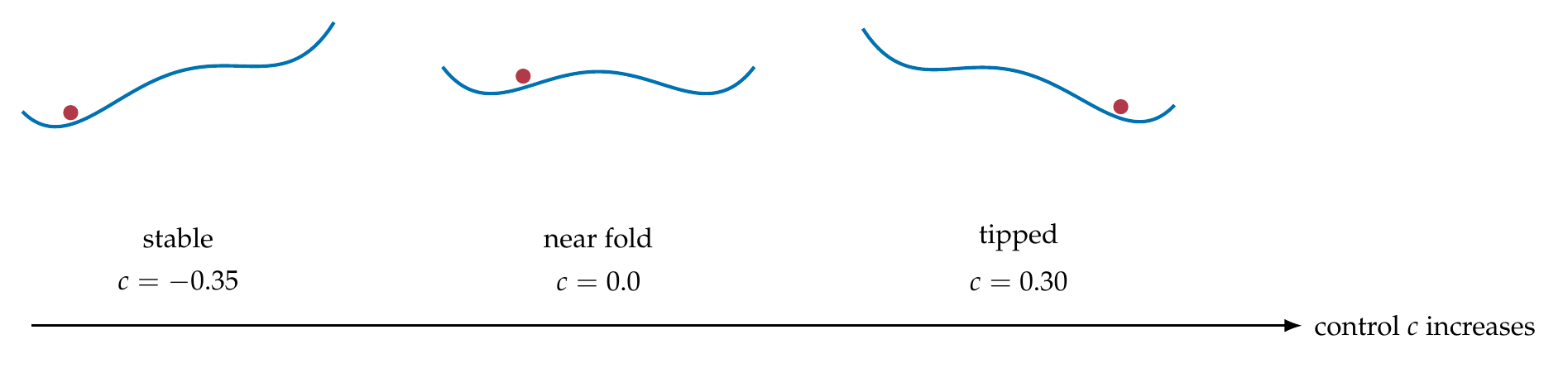
Note. The system is a ball in a potential landscape. Far from the transition (left) the ball sits in a deep well and returns quickly when nudged. As a control parameter drifts (center) the well the ball occupies grows shallow, so the ball returns sluggishly, critical slowing down. At the fold (right) that well vanishes and the ball rolls to the alternative state, the tip. The rising autocorrelation and variance of early-warning signals are the statistical shadow of the shallowing well.
The computation and its inference are where discipline is decisive. Early-warning indicators are computed in a rolling window over a detrended series, and the choices, the window width, the detrending method, are researcher degrees of freedom whose influence must be checked. The trend in an indicator is summarized by its Kendall rank correlation with time, and, crucially, that trend must be tested against a null that could have produced it by chance, because a rising autocorrelation can arise in any persistent series without any approaching transition. The null is built from surrogate series that share the observed autocorrelation but contain no trend toward a transition; comparing the observed Kendall trend to the distribution of trends in these surrogates yields an honest p-value. Figure 32.9 validates the whole pipeline on the bistable_sim series, generated from a genuine fold bifurcation in which a control parameter drifts slowly past the tipping point. The indicators rise as the theory predicts, the autocorrelation trend (\(\tau = 0.51\)) and the variance trend (\(\tau = 0.47\)) are both significant against the surrogate null (\(p < 0.001\) and \(p = 0.01\)), and the warning leads the tip by a long margin. This is the method working as advertised, on clean data from a known transition.
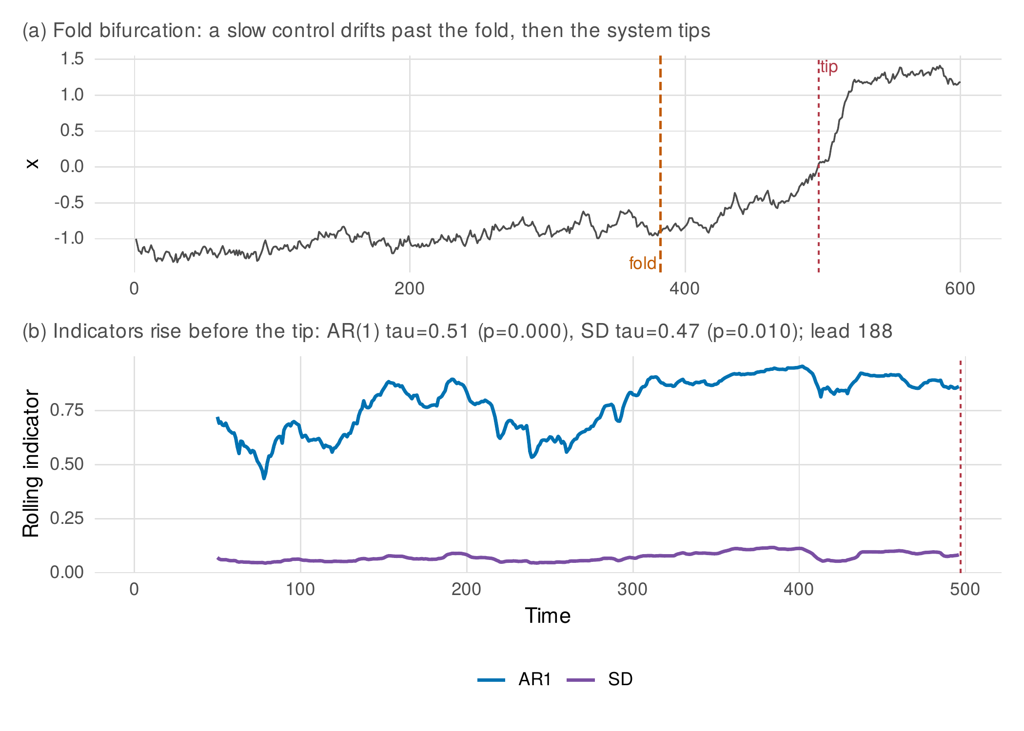
Note. Panel (a): the bistable_sim series, generated from a genuine fold bifurcation, sits in the lower state as a control parameter drifts past the fold (orange) and then tips to the upper state (red). Panel (b): the rolling lag-one autocorrelation and standard deviation rise before the tip, as critical-slowing-down theory predicts; both trends are significant against an autocorrelation-matched surrogate null, and the warning leads the tip by a long margin. On clean data from a known transition, the method works.
The sobering exhibit follows, because real data are not clean and single cases are not populations. Figure 32.10 applies the same pipeline to the n1_mood series before the onset of its depressed regime. The verdict is mixed: the variance rises significantly (\(\tau = 0.71\), \(p = 0.008\)), but the autocorrelation, the more theoretically central indicator, does not (\(\tau = 0.44\), \(p = 0.11\)). And the deeper caution is not about this series’ particular result but about its status as a single, post-hoc case. A transition observed after the fact, in one person, with the analysis choices made knowing where the transition fell, is the weakest possible evidence for a prospective alarm, however clean the picture looks, because the base rate of transitions is low, the number of analysis choices is large, and a signal that appears before one transition tells us nothing about the false alarms it would raise before the many non-transitions. Table 32.4 defines the indicators and their failure modes, and Table 32.5 digests the state of the empirical evidence. The literature has celebrated single-case successes (van de Leemput et al., 2014; Wichers et al., 2016) and has met them with pointed critiques of base rates, window selection, and prospective performance (Bos & De Jonge, 2014), and the field’s prospective and replication record remains, as of this writing, genuinely mixed. The book’s verdict is correspondingly bounded: early-warning signals are a promising basis for hypothesis-generating monitoring, not a validated clinical alarm, and a claim that they anticipate an individual’s transition must be defended against the base-rate and analyst-degrees-of-freedom objections, not merely illustrated with a compelling case.
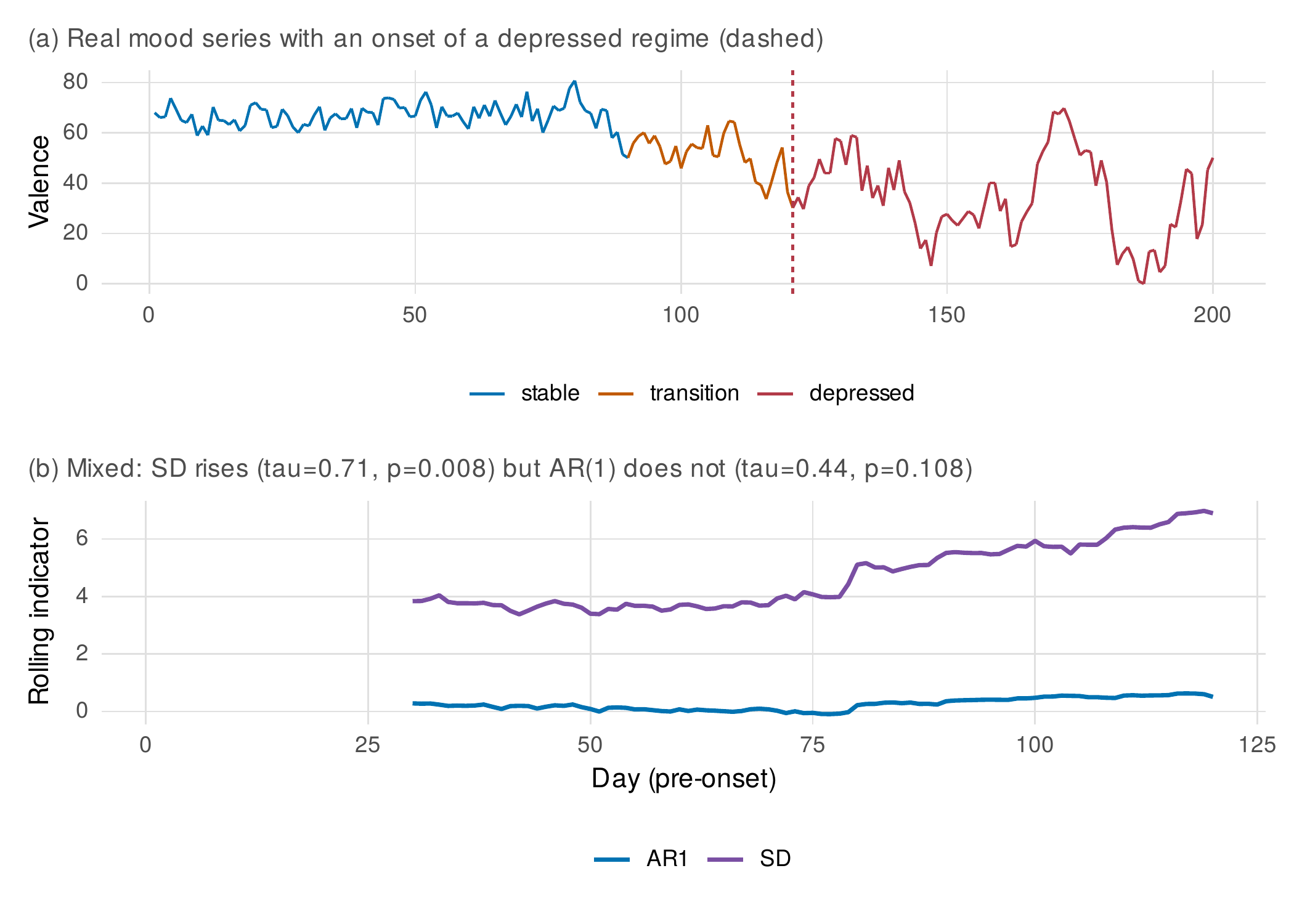
Note. The early-warning pipeline applied to the n1_mood series before its depressed-regime onset (dashed). The variance rises significantly (\(\tau = 0.71\), \(p = 0.008\)) but the autocorrelation does not (\(\tau = 0.44\), \(p = 0.11\)), a mixed verdict even before the deeper problem: this is a single, post-hoc case, the weakest evidence for a prospective alarm. Base rates and analyst degrees of freedom, not the appearance of a rising indicator, decide whether a warning is real.
Table 32.4. Early-Warning Indicators: Definition, Mechanism, Inference, Failure
| Indicator | Mechanism | Inference | Failure mode |
|---|---|---|---|
| Lag-1 autocorrelation | \(\phi=e^{-\kappa\Delta t}\to1\) as \(\kappa\to0\) | Kendall \(\tau\) vs surrogate null | Rises in any persistent series |
| Variance | \(\sigma^2/(2\kappa)\to\infty\) | Kendall \(\tau\) vs surrogate null | Rises with a changing mean too |
| Skewness/flickering | Asymmetric excursions near the fold | Surrogate null | Noisy; needs long series |
| Cross-correlation | Coupling strengthens near tip | Multivariate surrogate | Multiple-testing inflation |
Note. Each indicator has a mechanistic basis in critical slowing down and a characteristic failure mode. The window width and detrending are researcher degrees of freedom whose influence must be reported; the Kendall trend must be tested against a surrogate null; and multiple indicators tested together require multiplicity control. An indicator that rises is necessary, not sufficient, evidence for an approaching transition.
Table 32.5. Evidence Status for Early-Warning Signals in Psychopathology
| Claim | Status (as of this writing) |
|---|---|
| Celebrated single-case successes | Real and striking (e.g., a depression transition preceded by rising indicators), but post hoc |
| Mechanistic basis | Sound: critical slowing down is a genuine consequence of a fold bifurcation |
| Prospective performance | Mixed and contested; base-rate and false-alarm problems unresolved |
| Analyst degrees of freedom | Window and detrending choices materially affect results; preregistration rare |
| Clinical translation | Promising for monitoring; not a validated alarm |
Note. This digest is dated because the literature is active and contested; verify its current state at the time of use. The pattern to date is a sound theory with striking illustrative cases and an unsettled prospective record. The defensible claim is monitoring for hypothesis generation, not prediction of an individual’s transition.
In Practice • Convergence craft and surrogate implementation
Two practical matters recur across the chapter’s methods. Fitting regime-switching and nonlinear state-space models is a starting-value problem, as it was in Chapters 22 and 26: local maxima and label switching are the norm, so a fit should be launched from many starting points, the best retained, and the regime labels fixed by an ordering convention (here, increasing state mean) before interpretation. The dynr package exposes the same convergence controls as the state-space fitting of Chapter 26, and its craft transfers. Surrogate inference, the backbone of honest early-warning and recurrence claims, has its own details: an autocorrelation-matched surrogate preserves the lag-one dependence of the series while destroying any trend in the indicator, so the observed Kendall trend is tested against what that dependence alone would produce; the surrogate must match the residual after detrending, not the raw series, and the number of surrogates (several hundred) sets the resolution of the p-value. Both matters reward being scripted with fixed seeds, so that a reported p-value can be regenerated exactly.
32.5 Recurrence Quantification
Recurrence quantification is a descriptive lens on the structure of a dynamical series, and it earns a place here as a nonlinear complement to the autocorrelation-based descriptions of earlier chapters. The recurrence plot marks every pair of times at which the system revisits a similar state, after embedding the series to reconstruct its state space, and the visual texture of that plot distinguishes dynamical regimes: a periodic system produces long diagonal lines, because a state recurs at regular intervals; a stochastic system produces a scattered, textureless plot. Recurrence quantification analysis turns the texture into numbers, the recurrence rate, the determinism (the fraction of recurrence points lying on diagonal lines, indexing predictability), and the laminarity (the fraction on vertical lines, indexing trapping in states). Figure 32.11 contrasts a sustained oscillation with an autocorrelated noise series of the same length: the oscillation’s recurrence plot is ruled with long diagonals and its determinism is high (\(0.87\)), the noise series is scattered and its determinism lower (\(0.70\)), and the difference is significant against a surrogate null (\(p < 0.001\)). The framing must stay descriptive: recurrence metrics characterize a series, and any inferential claim built on them, that two series differ in determinism, that a dyad’s coordination exceeds chance, requires a surrogate test, exactly as here. Recurrence quantification is at its most valuable for the coordination of coupled series, the synchrony of a conversing dyad, a use the applications chapters develop.
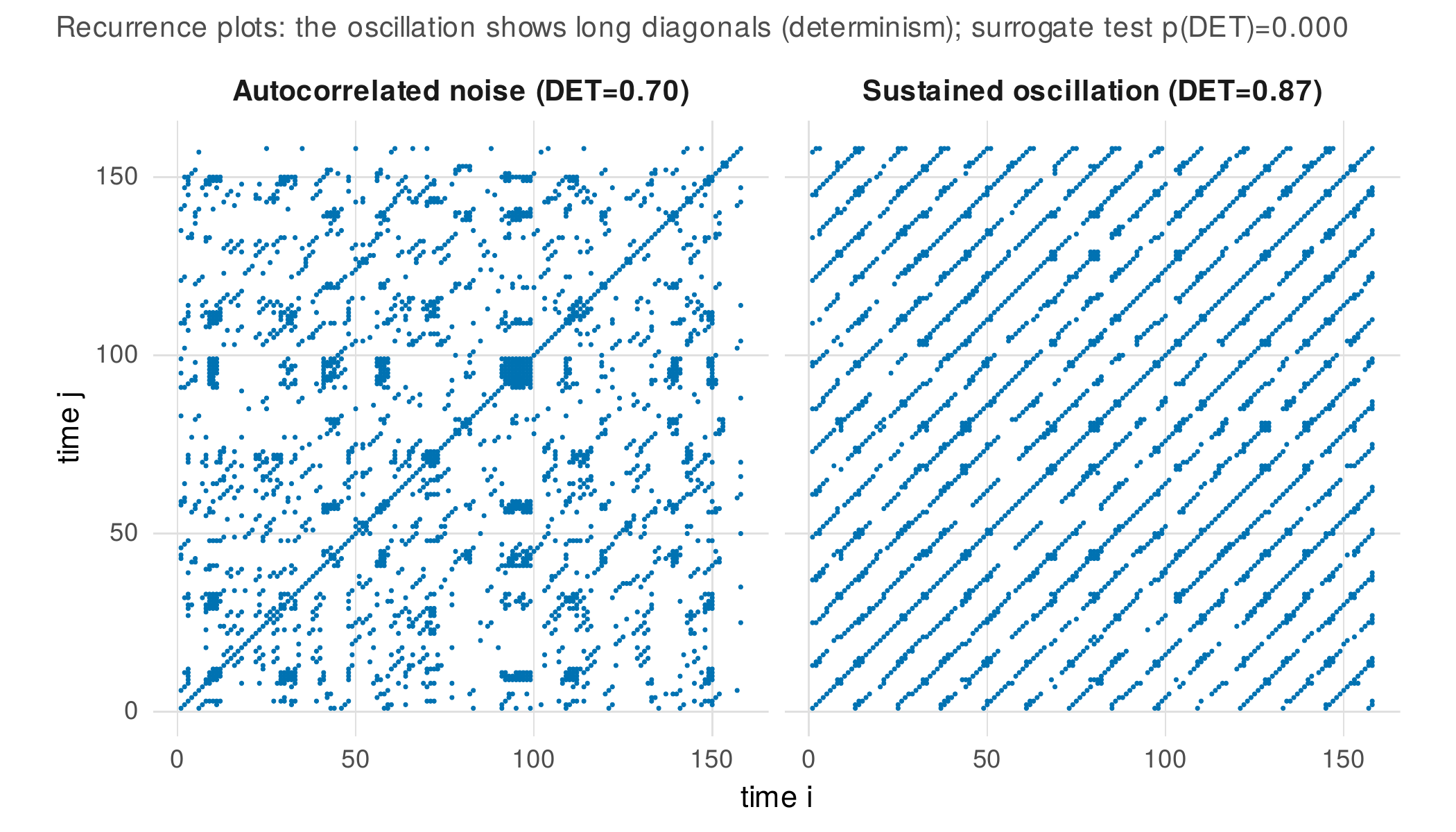
Note. Recurrence plots for an autocorrelated noise series (left) and a sustained oscillation (right) of the same length. A recurrence point marks two times at which the system occupies a similar state. The oscillation’s long diagonal lines are the signature of periodic determinism; the noise series is scattered. The determinism metric quantifies the difference (\(0.87\) versus \(0.70\)), and it is significant against a surrogate null (\(p < 0.001\)). Recurrence quantification is descriptive; inferential claims from it require surrogate testing.
32.6 The Honesty Ledger
The chapter’s methods span a wide range of data demands and evidential warrant, and the frontier is exactly where a frank accounting of that range does the most good. Figure 32.12 and Table 32.6 are that accounting: a ledger of which nonlinear method is defensible at which data budget, and what claim each supports. A two-state hidden Markov model can be workable with a hundred occasions and well-supported with several hundred; a Markov-switching autoregression needs more, because it estimates dynamics within each regime; oscillator estimation is fragile below a few hundred occasions and its claims are bounded by the embedding sensitivity regardless of length; single-series early-warning inference is workable only with long records and, even then, supports monitoring rather than prediction; and recurrence quantification, being descriptive, is usable earlier but claims less. The ledger’s discipline is to match the claim to the budget and to report, for any nonlinear analysis, the sensitivity of the conclusion to the analyst’s choices, the window and detrending for early-warning signals, the embedding for oscillators and recurrence, the starting values and regime number for switching models. A nonlinear result reported without that sensitivity is not yet a finding. The chapter’s exciting machinery and its sobering ledger are not in tension; on this frontier, the ledger is what makes the machinery usable.
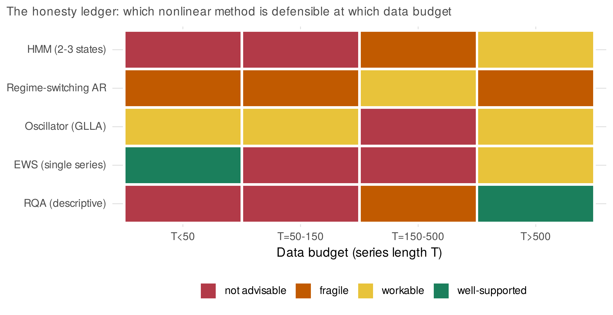
Note. A capability ledger for the chapter’s methods against the length of the series. Regime-switching models and recurrence quantification are usable at modest lengths; Markov-switching autoregressions and oscillator estimation need longer records and remain fragile; single-series early-warning inference is workable only with long records and supports monitoring, not prediction. The ledger encodes the chapter’s central discipline: match the claim to the data budget, and report the sensitivity of every nonlinear conclusion to the analyst’s choices.
Table 32.6. The Honesty Ledger: Method, Minimum Data, Claim Ceiling
| Method | Minimum \(T\) | Claim ceiling |
|---|---|---|
| HMM (2–3 states) | \(\sim\)100 | Regimes as validated hypotheses, not proven types |
| Markov-switching AR | \(\sim\)200 | Regime-specific dynamics with wide uncertainty |
| Oscillator (GLLA) | \(\sim\)200 | Oscillation only with visible cycle + robustness |
| Early-warning signals | \(\gg\)200, single case weak | Monitoring hypotheses, not prospective alarms |
| Recurrence quantification | \(\sim\)100 | Descriptive structure; inference needs surrogates |
Note. Minimum lengths are rough and generous; genuine identification often needs more. The claim ceiling is the strongest defensible conclusion, and it is well below what the enthusiastic literature sometimes asserts. The universal requirement is a sensitivity analysis across the analyst’s degrees of freedom; without it, no nonlinear conclusion is secure.
Common Pitfall • Four ways to see nonlinearity that is not there
Regimes from outliers. A two-state model will assign a handful of extreme points to a second “regime” that is only heavy-tailed noise; check the enumeration and the posterior uncertainty. Early-warning signals from window shopping. Trying many window widths and detrending choices until an indicator rises manufactures a warning; fix the choices in advance and report the sensitivity. Oscillations from smoothing artifacts. Smoothing a series before estimating derivatives can induce spurious periodicity; the oscillator must be visible in the raw data. Hysteresis from asymmetric means. A difference between an up-phase mean and a down-phase mean is not hysteresis unless the state genuinely depends on history; a static difference in level is not a loop.
Software Note • A patchy ecosystem, stated plainly
The software for nonlinear dynamics in psychology is uneven, and candor serves readers. The dynr package fits regime-switching and nonlinear state-space models and is the maintained tool for the models of Section 32.2; depmixS4 fits hidden Markov models. Oscillator estimation by generalized local linear approximation has no single canonical package and is often hand-coded, as here. Early-warning-signal tools have existed (an earlywarnings package and its relatives) but their maintenance is intermittent, so the indicators and their surrogate tests are frequently, and reasonably, hand-built; the pipeline in this chapter’s companion is a documented, reusable implementation with surrogate inference included. Recurrence quantification is served by crqa for cross-recurrence. Because several of these were unavailable in the environment that produced this chapter, the hidden Markov model, the oscillator estimation, the early-warning pipeline with its surrogate null, and recurrence quantification are all hand-coded on base R, which both guarantees reproducibility and makes plain that the methods are more transparent than their tooling suggests.
Chapter Summary
Nonlinear dynamics extends the book to phenomena its linear default cannot represent, switches, cycles, hysteresis, and transitions between alternative stable states, and it does so on the frontier where the gap between promise and evidence is widest, so every method is paired with the discipline that keeps it honest. Nonlinearity is a substantive claim warranted by a signature a linear model cannot produce, not a decoration, and three formalisms handle the signatures: discrete regimes, continuous flows, and critical transitions. Regime-switching models suppose the system occupies one of a few hidden states with its own dynamics: a three-state hidden Markov model recovers the planted regimes of a mood series with posterior uncertainty reported honestly, and a Markov-switching autoregression shows the depressed regime to be both more persistent and more volatile, dysregulation in the dynamics themselves. But a two-state model fits heavy-tailed single-regime noise as readily as genuine regimes, so the enumeration discipline of Chapter 22 governs: a recovered regime is a hypothesis validated externally, not a discovered type. Differential-equation models formalize regulation as a restoring force, and the damped linear oscillator gives frequency and damping a reading as the tempo and thoroughness of a return to equilibrium; generalized local linear approximation recovers a known oscillator but its estimates drift with the embedding dimension, and on real data the oscillator fits nearly everyone because mean reversion mimics oscillation, so the honest report is the embedding-sensitivity curve and the demand for a visible cycle, not a point estimate. Critical-transition theory predicts that a system approaching a fold bifurcation slows down, its autocorrelation and variance rising, a consequence of the vanishing recovery rate derived cleanly from the linearized dynamics; the early-warning pipeline, computed in rolling windows and tested against autocorrelation-matched surrogates, detects the transition in a known fold-bifurcation series with a long lead time, but on a single real mood series gives a mixed verdict and, more importantly, is post hoc, so the defensible claim is monitoring for hypothesis generation, not a validated prospective alarm. Recurrence quantification describes dynamical structure, distinguishing a deterministic oscillation from noise by its determinism with a surrogate test, and stays descriptive. The honesty ledger consolidates the frontier’s discipline: match the claim to the data budget, report the sensitivity of every nonlinear conclusion to the analyst’s degrees of freedom, and recognize that on this frontier the ledger is not a hedge but the condition of using the machinery at all.
Boker, S. M., & Nesselroade, J. R. (2002). A method for modeling the intrinsic dynamics of intraindividual variability: Recovering the parameters of simulated oscillators in multi-wave panel data. Multivariate Behavioral Research, 37(1), 127–160. https://doi.org/10.1207/S15327906MBR3701_06
Bos, E. H., & De Jonge, P. (2014). “Critical slowing down in depression” is a great idea that still needs empirical proof. Proceedings of the National Academy of Sciences, 111(10), Article E878. https://doi.org/10.1073/pnas.1323672111
Chow, S.-M., Ferrer, E., & Nesselroade, J. R. (2007). An unscented Kalman filter approach to the estimation of nonlinear dynamical systems models. Multivariate Behavioral Research, 42(2), 283–321. https://doi.org/10.1080/00273170701360423
Chow, S.-M., Ram, N., Boker, S. M., Fujita, F., & Clore, G. (2005). Emotion as a thermostat: Representing emotion regulation using a damped oscillator model. Emotion, 5(2), 208–225. https://doi.org/10.1037/1528-3542.5.2.208
Chow, S.-M., & Zhang, G. (2013). Nonlinear regime-switching state-space (RSSS) models. Psychometrika, 78(4), 740–768. https://doi.org/10.1007/s11336-013-9330-8
Coco, M. I., & Dale, R. (2014). Cross-recurrence quantification analysis of categorical and continuous time series: An R package. Frontiers in Psychology, 5, Article 510. https://doi.org/10.3389/fpsyg.2014.00510
Dakos, V., Carpenter, S. R., Brock, W. A., Ellison, A. M., Guttal, V., Ives, A. R., Kéfi, S., Livina, V., Seekell, D. A., van Nes, E. H., & Scheffer, M. (2012). Methods for detecting early warnings of critical transitions in time series illustrated using simulated ecological data. PLoS ONE, 7(7), Article e41010. https://doi.org/10.1371/journal.pone.0041010
Deboeck, P. R. (2010). Estimating dynamical systems: Derivative estimation hints from Sir Ronald A. Fisher. Multivariate Behavioral Research, 45(4), 725–745. https://doi.org/10.1080/00273171.2010.498294
Hamaker, E. L., & Grasman, R. P. P. P. (2012). Regime switching state-space models applied to psychological processes: Handling missing data and making inferences. Psychometrika, 77(2), 400–422. https://doi.org/10.1007/s11336-012-9254-8
Haslbeck, J. M. B., & Ryan, O. (2022). Recovering within-person dynamics from psychological time series. Multivariate Behavioral Research, 57(5), 735–766. https://doi.org/10.1080/00273171.2021.1896353
Marwan, N., Romano, M. C., Thiel, M., & Kurths, J. (2007). Recurrence plots for the analysis of complex systems. Physics Reports, 438(5–6), 237–329. https://doi.org/10.1016/j.physrep.2006.11.001
Olthof, M., Hasselman, F., Strunk, G., van Rooij, M., Aas, B., Helmich, M. A., Schiepek, G., & Lichtwarck-Aschoff, A. (2020). Critical fluctuations as an early-warning signal for sudden gains and losses in patients receiving psychotherapy for mood disorders. Clinical Psychological Science, 8(1), 25–35. https://doi.org/10.1177/2167702619865969
Ou, L., Hunter, M. D., & Chow, S.-M. (2019). What’s for dynr: A package for linear and nonlinear dynamic modeling in R. The R Journal, 11(1), 91–111. https://doi.org/10.32614/RJ-2019-012
Scheffer, M., Bascompte, J., Brock, W. A., Brovkin, V., Carpenter, S. R., Dakos, V., Held, H., van Nes, E. H., Rietkerk, M., & Sugihara, G. (2009). Early-warning signals for critical transitions. Nature, 461(7260), 53–59. https://doi.org/10.1038/nature08227
Scheffer, M., Carpenter, S. R., Lenton, T. M., Bascompte, J., Brock, W., Dakos, V., van de Koppel, J., van de Leemput, I. A., Levin, S. A., van Nes, E. H., Pascual, M., & Vandermeer, J. (2012). Anticipating critical transitions. Science, 338(6105), 344–348. https://doi.org/10.1126/science.1225244
Thelen, E., & Smith, L. B. (1994). A dynamic systems approach to the development of cognition and action. MIT Press.
van de Leemput, I. A., Wichers, M., Cramer, A. O. J., Borsboom, D., Tuerlinckx, F., Kuppens, P., van Nes, E. H., Viechtbauer, W., Giltay, E. J., Aggen, S. H., Derom, C., Jacobs, N., Kendler, K. S., van der Maas, H. L. J., Neale, M. C., Peeters, F., Thiery, E., Zachar, P., & Scheffer, M. (2014). Critical slowing down as early warning for the onset and termination of depression. Proceedings of the National Academy of Sciences, 111(1), 87–92. https://doi.org/10.1073/pnas.1312114110
Wichers, M., Groot, P. C., Psychosystems, ESM Group, & EWS Group. (2016). Critical slowing down as a personalized early warning signal for depression. Psychotherapy and Psychosomatics, 85(2), 114–116. https://doi.org/10.1159/000441458