Chapter 33
Applications in Clinical Psychology and Mental Health
The preceding chapters built a toolkit one method at a time, and a toolkit is not yet a practice. This chapter, the first of the applications part, shows the methods working together on real clinical questions, because the decisions that matter most in an actual study are decisions about integration: which analysis answers the question, in what order the analyses should run, how they corroborate or contradict one another, and how the whole is reported so that a reviewer, a regulator, and a clinician can each read it. Three case studies carry the argument, each written as an empirical paper would be written, with a running commentary that exposes the reasoning a finished paper conceals. The first takes a depression trial seriously: it models the treatment’s effect on the symptom trajectory, converts that effect into the remission outcome a clinician cares about, confronts the substantial dropout that threatens every trial’s conclusions, and subjects the finding to the missing-data sensitivity analyses that turn a fragile claim into a robust one, treating the sensitivity analysis not as an appendix but as a first-class result. The second studies symptom dynamics in intensive longitudinal data and insists on a discipline the enthusiasm for such data often forgets: the same data can be represented as a multilevel model, a dynamic network, and an idiographic portrait, and these are three lenses on one truth that must be reconciled rather than three competing findings to be reported selectively. The third addresses the newest clinical activity, the delivery of interventions through a phone, and separates three things that digital mental health routinely conflates: optimizing an intervention by micro-randomization, predicting risk by machine learning, and monitoring for transitions by early-warning signals, each a different estimand with a different standard of evidence. The unifying commitments are the book’s throughout: visualize first, name the estimand first, and analyze the sensitivity always.
Learning Objectives
After working through this chapter, you should be able to: (1) translate clinical questions into estimands and the chapter-mapped analyses that address them; (2) sequence multiple analyses on one dataset with principled logic rather than kitchen-sink reporting; (3) handle the realities of clinical longitudinal data, including symptom-dependent dropout, therapist nesting, and assessment reactivity; (4) conduct and report missing-data sensitivity analyses as a clinical-evidence obligation; (5) reconcile multiple representations of intensive longitudinal data; (6) distinguish intervention optimization, risk prediction, and anomaly monitoring as separate digital-mental-health activities; and (7) write clinical longitudinal results that a reviewer, a regulator, and a clinician can each read.
33.1 Clinical Longitudinal Research: The Terrain
Clinical questions about change fall into a handful of families, and each family routes to a part of this book. Whether a treatment works, and how fast, is a question about symptom trajectories, answered by the growth models of Chapters 13, 14, and 19. For whom it works is a question about heterogeneity, approached with the guarded mixture models of Chapter 22 and the tree methods of Chapter 31. Who relapses, and when, is a timing question, answered by the survival models of Chapter 29. How symptoms interact within a patient is a dynamics question, answered by the multilevel vector-autoregression and network methods of Chapters 25 and 28. Whether an impending deterioration can be seen coming is a monitoring question, approached with the state-space and nonlinear methods of Chapters 26 and 32, with all their cautions. And how to deliver an intervention at the right moment is an optimization question, answered by the micro-randomized designs this chapter introduces. Figure 33.1 draws the routing, and Table 33.1 sets it out with the estimands and exemplar literatures.
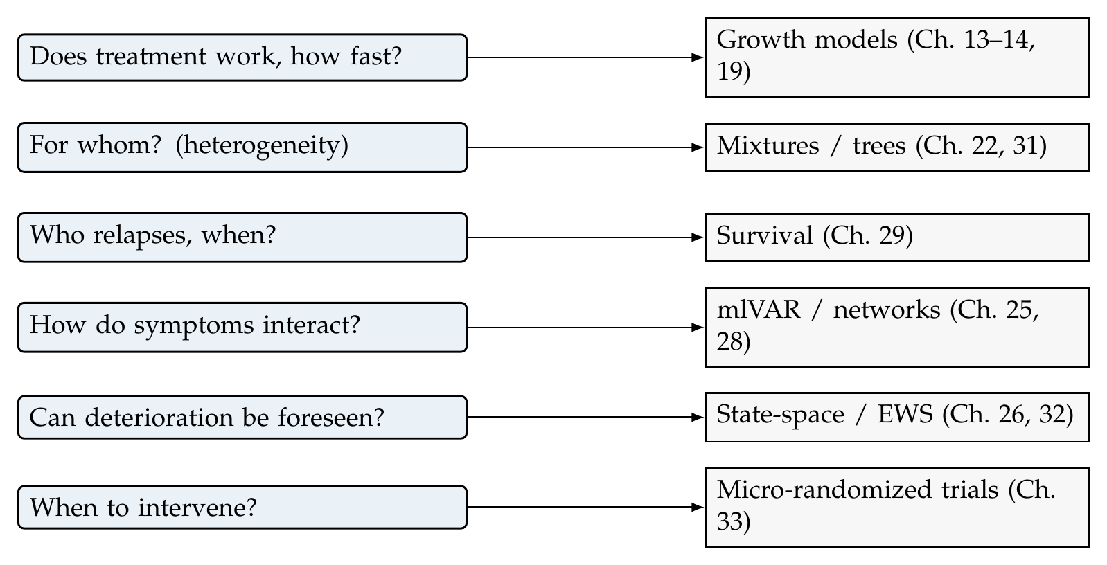
Note. Each family of clinical question routes to the part of the book that answers it. The routing is estimand-first: the question determines the method, not the reverse. A single study usually asks several of these questions, and the integration of the corresponding analyses, in a principled sequence with honest reconciliation, is the subject of this chapter’s case studies.
Table 33.1. Clinical Question Taxonomy, Estimands, and Chapters
| Question | Estimand | Chapters (exemplars) |
|---|---|---|
| Efficacy trajectory | Arm difference in change | 13–14, 19 (Gueorguieva & Krystal, 2004) |
| Heterogeneity | Subgroup or class effects | 22, 31 |
| Relapse timing | Hazard of the event | 29 |
| Within-patient dynamics | Lagged and contemporaneous effects | 25, 28 (Bringmann et al., 2013) |
| Monitoring | Change in stability over time | 26, 32 |
| Delivery optimization | Causal excursion effect | 33 (Klasnja et al., 2015) |
Note. The estimand column is the discipline: a clinical question is answerable only once its target of inference is named. Several rows usually apply to one study, and the analyst’s task is to sequence them, letting each inform the next, rather than to run all methods and report the most flattering.
Three realities of clinical longitudinal data shape every analysis that follows. Symptom scales may not measure the same construct the same way as treatment proceeds, a response shift that the invariance methods of Chapter 18 can test and that undermines a naive comparison of scores across time if ignored. Frequent assessment of symptomatic patients carries burden and reactivity, so the measurement schedule is an ethical and estimand question, not merely a logistical one. And patients are nested in therapists and sites, a multilevel structure that inflates false-positive rates if unmodeled. To these the trials tradition adds a discipline psychology is still absorbing: the estimand framework of the ICH E9(R1) addendum, which insists that the handling of dropout and rescue medication be specified as part of the estimand itself, so that a treatment-policy strategy (the effect regardless of adherence), a hypothetical strategy (the effect had all patients adhered), and a while-on-treatment strategy answer genuinely different questions and must not be conflated. Table 33.2 translates these strategies for the psychologist, and Case Study A puts them to work.
Table 33.2. Estimand Strategies for Dropout and Rescue (ICH E9(R1), Translated)
| Strategy | The question it answers | Handling of dropout |
|---|---|---|
| Treatment policy | Effect of being assigned, regardless of adherence | Follow up all, including after discontinuation |
| Hypothetical | Effect had everyone adhered | Model the counterfactual (e.g., FIML under MAR) |
| While on treatment | Effect during the period on treatment | Analyze up to discontinuation |
| Composite | Discontinuation is itself a poor outcome | Combine with the outcome |
Note. The strategies answer different clinical questions and yield different estimates; the choice must precede the analysis and be reported as part of the estimand. The mixed model under missing-at-random targets a hypothetical strategy; the sensitivity analyses of Case Study A probe how far a missing-not-at-random departure would move that estimate.
33.2 Case Study A: The Trial, Taken Seriously
The therapy_rct data are a randomized trial of two hundred forty patients, half assigned to an active treatment and half to control, with the Hamilton depression rating scale measured weekly for twelve weeks. The analysis proceeds in a deliberate sequence, each step motivated by the last, and Table 33.3 is the decision log that records the reasoning, the reproducible-reasoning exhibit that a finished paper omits. Description and visualization come first, per the book’s standing rule. The primary analysis is a growth model of the symptom trajectory with a random intercept and slope, and its estimand is the difference between arms in the rate of change. The treatment arm improves faster, by half a Hamilton point per week more than control (\(-0.51\) points per week for the arm-by-time interaction), so that by week twelve the model-implied severity is \(8.5\) in the treatment arm against \(14.6\) in control, a difference that crosses the threshold from moderate to mild depression. A secondary generalized-linear mixed model translates the continuous trajectory into the outcome a clinician acts on, remission, defined as a Hamilton score below seven, and finds the odds of remission at week twelve many times higher under treatment. Figure 33.2 shows the trajectories and, beneath them, the fact that threatens the whole conclusion.
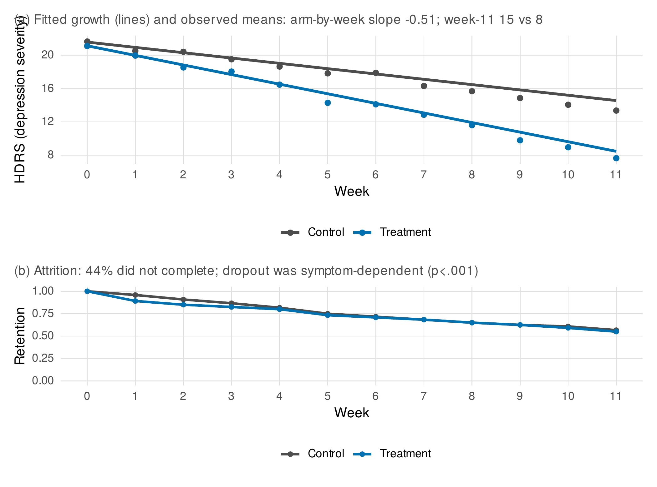
Note. Panel (a): the fitted growth model (lines) and observed weekly means (points) for the therapy_rct trial. The treatment arm improves faster (arm-by-week slope \(-0.51\)), reaching a model-implied Hamilton score of \(8.5\) at week twelve against \(14.6\) in control. Panel (b): retention falls to about fifty-five percent by week twelve, and the dropout is symptom-dependent, patients with higher current symptoms are likelier to leave. Attrition of this magnitude and this mechanism can bias the primary estimate, which is why the sensitivity analysis is not optional.
That fact is attrition. Forty-four percent of patients did not complete the trial, and a discrete-time hazard model of dropping out shows the dropout to be symptom-dependent: patients with higher current symptoms are more likely to leave (\(p < .001\)). The primary growth model, fit by full-information maximum likelihood, is valid if the dropout is missing at random given the observed trajectory, which the symptom-dependence makes plausible but not certain, because the value that triggers dropout is the one that goes unobserved. This is the missing-not-at-random worry of Chapter 6, and the clinical-evidence obligation is to probe it, not to assert it away. Two sensitivity analyses do so, and Figure 33.3 displays them. A tipping-point analysis imputes each dropout’s missing scores from the model and then penalizes the treatment-arm dropouts by adding a fixed number of Hamilton points, on the hypothesis that treated patients who leave fare worse than the model predicts; sweeping that penalty from zero to eight points, the treatment benefit attenuates but remains significant throughout, so it would take an implausibly large and arm-specific departure from missing-at-random to overturn the conclusion. A shared-parameter joint model, which fits the trajectory and the dropout process together with a shared random slope, reaches the same estimate as the naive model (\(-0.512\) against \(-0.514\)) and finds the dropout only weakly associated with the slope, corroborating the missing-at-random assumption directly. The two sensitivity analyses converge, and that convergence, not the primary estimate alone, is the robust finding.
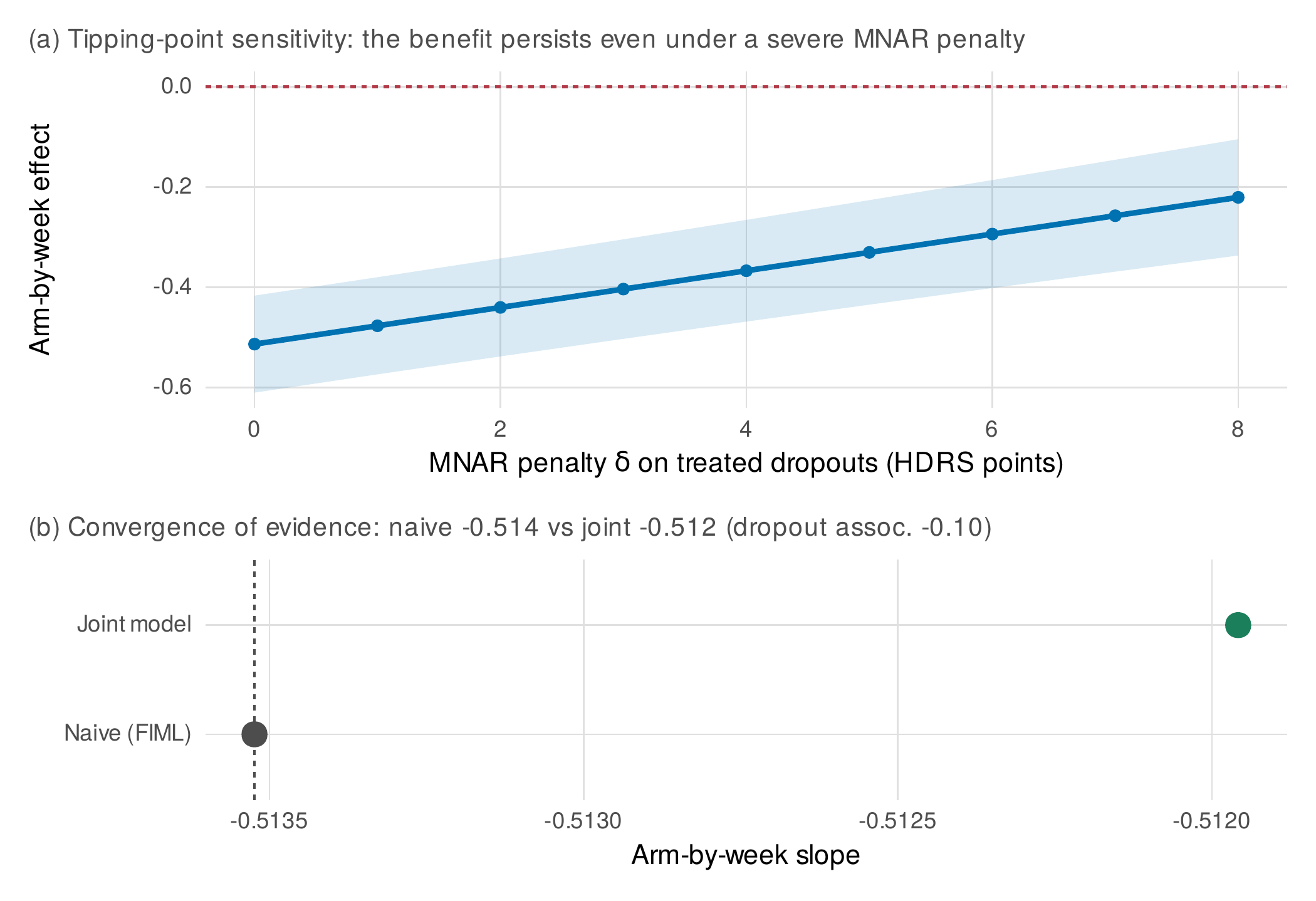
Note. Panel (a): a tipping-point analysis penalizes treatment-arm dropouts by a fixed number of Hamilton points (the horizontal axis) and refits; the arm-by-week benefit attenuates but stays significant even under an eight-point penalty, so overturning it requires an implausible missing-not-at-random departure. Panel (b): a shared-parameter joint model of trajectory and dropout reaches essentially the naive estimate (\(-0.512\) versus \(-0.514\)) with a near-zero dropout association, corroborating missing-at-random. The convergence of the two analyses is the robust conclusion.
A final, honestly labeled step asks whether the average effect hides responder heterogeneity. An exploratory growth mixture identifies two latent trajectory classes, a fast-responding group and a slow-responding one, but the analysis is reported with every guardrail of Chapter 22: the classes are described as an exploratory hypothesis, their number is not treated as discovered, and they are not reified into clinical subtypes on the strength of a single sample. The teaching payload of the whole case is the sequencing, description before modeling, primary before secondary, and sensitivity as obligation, and the translation of a trajectory difference into the remission language a clinical audience needs.
Table 33.3. Case Study A: The Analysis-Sequencing Decision Log
| # | Step | Reasoning |
|---|---|---|
| 1 | Visualize and describe | See trajectories and attrition before modeling (book rule) |
| 2 | Primary growth model | Arm-by-time estimand; the pre-specified question |
| 3 | Remission GLMM | Translate the trajectory into a clinical outcome |
| 4 | Dropout hazard | Diagnose the missingness mechanism before trusting step 2 |
| 5 | Tipping-point sensitivity | Quantify how much MNAR departure would overturn the result |
| 6 | Joint model | Corroborate MAR by modeling dropout and trajectory jointly |
| 7 | Exploratory mixture | Probe heterogeneity, guarded and unreified |
Note. The log is the pedagogical artifact a finished paper omits: it records why each analysis followed the last. Steps 4 through 6 exist because step 2’s validity depends on an untestable assumption, and the sensitivity analyses convert that dependence into a bounded, reported uncertainty rather than an unstated risk.
33.3 Case Study B: Symptom Dynamics and Personalized Structure
The affect_ema data follow a sample through many days of ecological momentary assessment, and the clinical interest is in the dynamics: how a patient’s stress spills over into negative affect, how affect carries forward, and how these dynamics differ across patients. The analysis begins with measurement and description, because momentary items are noisier than questionnaire scales: a multilevel reliability analysis shows that thirty-six percent of the variance in momentary negative affect lies between persons, and the dynamic indices of Chapter 7, a mean autocorrelation of \(0.37\) and a mean successive difference of \(0.60\), describe the tempo and instability of the series before any model is imposed. The primary dynamic analysis is a multilevel vector-autoregression, which estimates each variable’s dependence on the recent past of itself and the others, with random effects that let the dynamics differ by person. It finds a clear stress-to-affect spillover, a lagged effect of stress on negative affect of \(0.24\), and an affective inertia, a carry-forward of negative affect, of \(0.31\), both varying across patients.
The discipline the case study exists to teach is that these dynamics can be represented three ways, and the three are one truth seen through different lenses, to be reconciled rather than reported selectively. The multilevel model states the effects as regression coefficients with random variation. The same lagged coefficients, arranged as a matrix, are a temporal network whose directed edges are exactly those coefficients, the representation of Chapter 28. And the random effects are the raw material for idiographic portraits of individual patients. Figure 33.4 shows the first two lenses together, the temporal network of fixed effects and the distribution of person-specific spillovers, and Table 33.4 reconciles what each lens claims. The network figure must carry the claims-ladder discipline of Chapter 28: its edges are conditional associations, not proven mechanisms, and a centrality claim requires the stability analysis that chapter mandated. The reconciliation is the point. A paper that presented the network as a new finding beside the multilevel model, as though they were separate results, would be double-counting one analysis; a paper that presented only the network, with its vivid picture, would be hiding the uncertainty the coefficients carry.
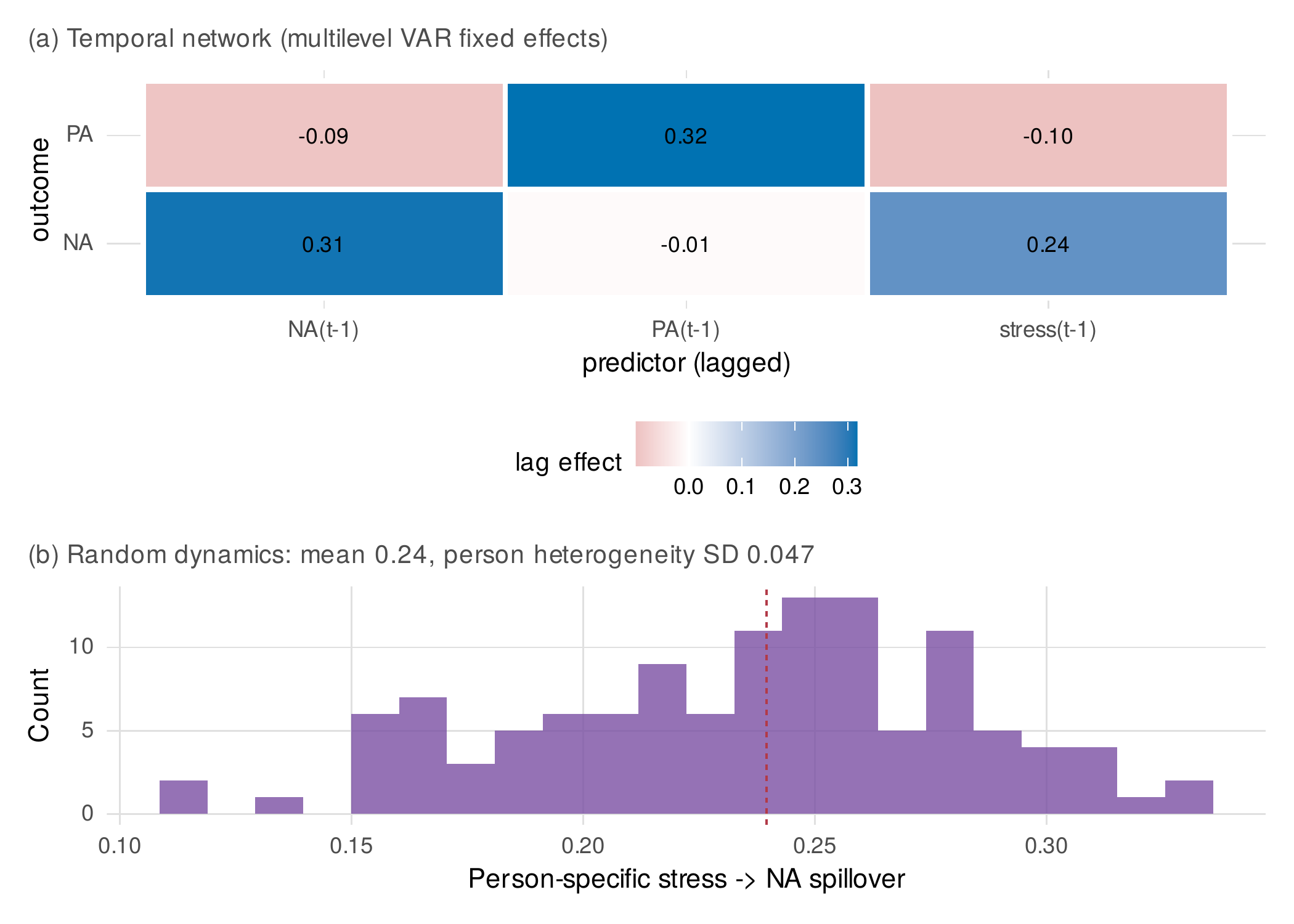
Note. Panel (a): the temporal network of the affect_ema dynamics as the lagged fixed-effect matrix of a multilevel vector-autoregression; a directed edge is a lagged coefficient, a conditional association and not a proven mechanism. Panel (b): the person-specific stress-to-affect spillover varies across patients around its mean of \(0.24\), the random dynamics that a single average would hide. The network and the multilevel model are one analysis in two representations, to be reconciled, not reported as separate findings.
Idiographic analysis then asks what can be said about an individual patient, and here the pooling lesson of Chapter 25 returns with clinical stakes. Figure 33.5 contrasts, for two patients, the person-specific estimate computed from that patient’s data alone with the shrunken estimate the multilevel model assigns. For a patient with ample, consistent data the two agree closely; for a patient with noisier data they diverge substantially, the multilevel model pulling the unstable individual estimate toward the group. Reporting the person-specific number alone would over-trust a noisy estimate; reporting the shrunken number alone would understate genuine individuality. The clinical translation must be correspondingly careful: a person-specific dynamic is a hypothesis about that patient to be checked against their history and their clinician’s knowledge, not a validated individual fact, and the ethics of reporting it, the patient’s privacy, the temptation to over-interpret a single striking coefficient, are part of the analysis, not an afterthought.
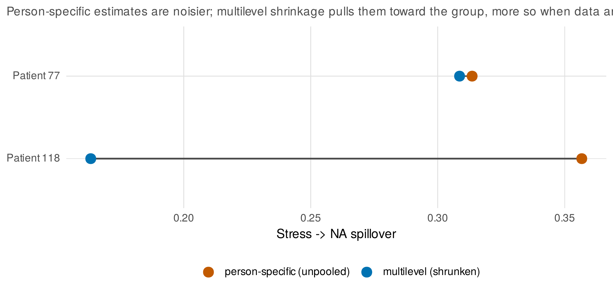
Note. For two patients, the stress-to-affect spillover estimated from that patient’s data alone (person-specific) and the estimate the multilevel model assigns after borrowing strength across patients (shrunken). For a patient with consistent data the two nearly coincide; for a patient with noisier data they diverge, the multilevel model regularizing the unstable individual estimate. The person-specific number over-trusts thin data; the shrunken number regularizes it. Neither is the whole story, and a clinical claim about an individual must acknowledge both.
Table 33.4. Case Study B: Reconciling the Representations
| Representation | What it claims | Relation to the others |
|---|---|---|
| Multilevel VAR | Lagged/contemporaneous coefficients with random variation | The estimation engine |
| Temporal network | Directed edges among variables | The same coefficients, drawn |
| Idiographic model | One patient’s own dynamics | The random effects, per person |
Note. The three are not independent findings but one analysis in three displays, and reporting them as though they corroborated one another would be double-counting. The network inherits the claims-ladder discipline of Chapter 28; the idiographic display inherits the shrinkage discipline of Chapter 25. One truth, reconciled across lenses, is the norm a clinical intensive-longitudinal paper should meet.
33.4 Case Study C: Monitoring, Prediction, and Just-in-Time Intervention
Digital mental health delivers assessment and intervention through a phone, and it routinely conflates three activities that are logically distinct: optimizing an intervention, predicting risk, and monitoring for transitions. The case study separates them, because each is a different estimand with a different design and standard of evidence, as Table 33.5 sets out. The just-in-time adaptive intervention, in the framework of Nahum-Shani et al. (2018), delivers support at decision points, tailored to the person’s momentary state, to affect a proximal outcome, and Figure 33.6 draws its architecture. The question it poses, does delivering the prompt now improve the proximal outcome, and for whom, is an intervention-optimization estimand, and the design that answers it is the micro-randomized trial, in which the intervention is randomized at each decision point so that its momentary causal effect is identified (Klasnja et al., 2015).
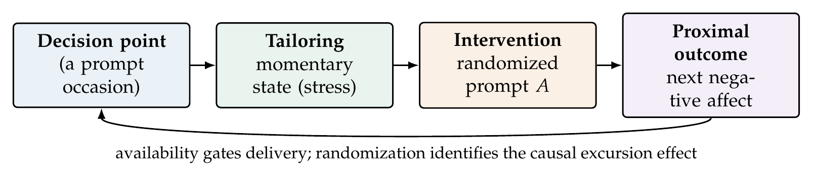
Note. At each decision point, a tailoring variable (the momentary state) informs whether an intervention is delivered, and the intervention affects a proximal outcome, feeding back into the next decision point. In a micro-randomized trial the intervention is randomized at each available decision point, which identifies the causal excursion effect, the momentary effect of delivering the prompt, averaged over the randomization distribution, and its moderation by the tailoring variable.
The mrt_ema data are a micro-randomized extension in which a brief coping prompt is randomized at each available decision point and the proximal outcome is the negative affect shortly after. The causal excursion effect is estimated by a weighted-and-centered regression that is robust to misspecification of the control model (Boruvka et al., 2018), and it recovers the planted effect: the prompt reduces proximal negative affect by about half a point when first delivered, its benefit wanes across the study as the person habituates, and it works more strongly when the person is stressed. Figure 33.7 shows the excursion effect over time, and the waning is itself the clinically actionable finding, because an intervention whose effect decays should be varied or spaced rather than repeated identically. This is optimization, not prediction: the estimand is the effect of an action, and the evidence is a randomized contrast.
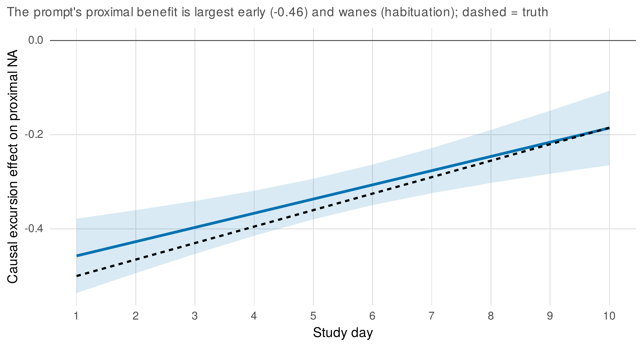
Note. The estimated causal excursion effect of the coping prompt on proximal negative affect in the mrt_ema micro-randomized trial, over study day, with the planted truth dashed. The prompt’s proximal benefit is largest when first delivered (about \(-0.46\)) and wanes across the study as the person habituates. The waning is the actionable result: an intervention whose momentary effect decays should be spaced or varied, a design conclusion only a micro-randomized trial can support.
Prediction is a different activity with a different estimand, the probability of a future state, and the discipline of Chapter 31 governs it. A risk-flag model forecasting momentary negative affect, evaluated by person-grouped cross-validation and measured against the persistence baseline, beats that baseline by a real but bounded margin (a cross-validated coefficient of determination of \(0.49\) against the baseline’s \(0.26\)), and its calibration must be checked, not merely its discrimination, as Figure 33.8 shows. Monitoring is a third activity, the detection of an approaching transition, and the early-warning verdict of Chapter 32 applies unchanged: a rising indicator in one patient’s stream is a monitoring hypothesis, not a validated alarm, and the base-rate and analyst-degrees-of-freedom cautions bind here as they did there. The teaching payload is the separation itself, because a digital-mental-health study that reports a predictive model as though it optimized an intervention, or an early-warning signal as though it predicted risk, has conflated three questions that require three designs.
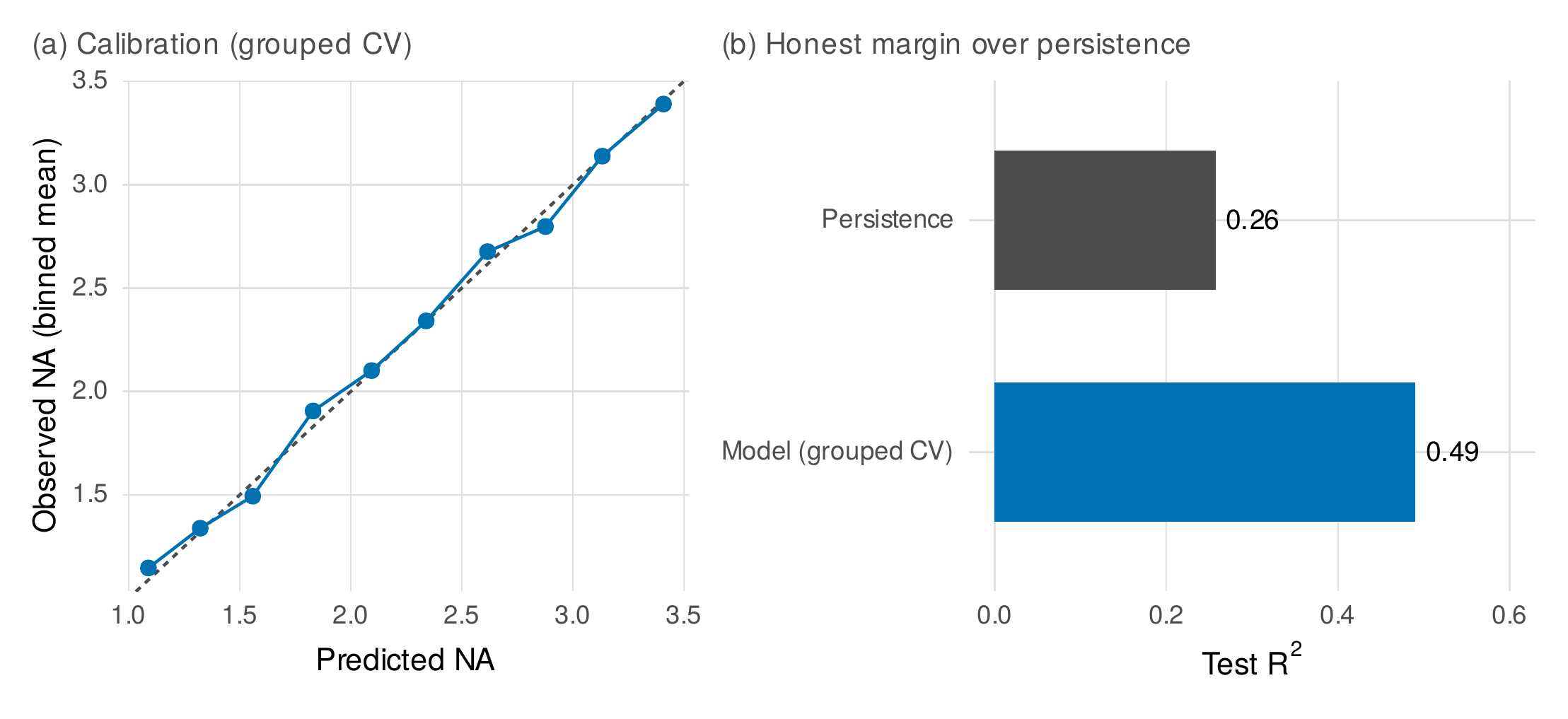
Note. Panel (a): the calibration of a person-grouped cross-validated model forecasting momentary negative affect, binned predicted against observed; points near the diagonal indicate good calibration. Panel (b): the model’s cross-validated coefficient of determination (\(0.49\)) against the persistence baseline (\(0.26\)), the honest margin. Prediction is judged by out-of-sample skill over a baseline and by calibration, not by in-sample fit, and it is a different activity from the intervention optimization of Figure 33.7.
Table 33.5. Three Digital-Mental-Health Activities, Distinguished
| Activity | Estimand | Design | Evidence |
|---|---|---|---|
| Optimization | Causal excursion effect | Micro-randomized trial | Randomized contrast |
| Prediction | Probability of a future state | Observational cohort | Grouped CV vs baseline |
| Monitoring | Change in stability | Intensive time series | Surrogate-tested trend |
Note. The three activities are routinely conflated in digital mental health, yet they answer different questions with different designs and standards. Optimization needs randomization; prediction needs honest out-of-sample evaluation; monitoring needs surrogate inference and base-rate humility. A study should name which it is doing and meet that activity’s standard.
33.5 Domain Synthesis
The three case studies share a spine, and naming it is the chapter’s synthesis. Each visualized before it modeled, named its estimand before it chose a method, and analyzed its sensitivity as a matter of course rather than on demand. Each also enforced a claims discipline particular to its methods: the trial bounded its conclusion with missing-data sensitivity, the dynamics study reconciled its representations rather than multiplying them, and the digital-health study separated optimization from prediction from monitoring. Figure 33.9 draws the clinical claims ladder that fixes the language a longitudinal result has earned to the evidence supporting it, and Table 33.6 is the reporting checklist a clinical journal should expect. The common reviewer objections to clinical longitudinal work, that the average effect is taken to settle what a treatment does for an individual, that more frequent measurement is assumed to be more clinical truth, that a network figure is read as a mechanism, that a forecast is oversold, are each answered by a discipline the case studies modeled. The domain literatures each add their own texture, the depression and anxiety ecological-momentary-assessment tradition (aan het Rot et al., 2012; Hamaker & Wichers, 2017), the experience-sampling study of psychosis (Myin-Germeys et al., 2009, 2018), the instability literature in borderline personality disorder (Trull et al., 2008; Ebner-Priemer & Trull, 2009), the idiographic-network exemplars (Fisher et al., 2017; Epskamp et al., 2018), but the analytic spine is common, and it is the spine this book has built toward.
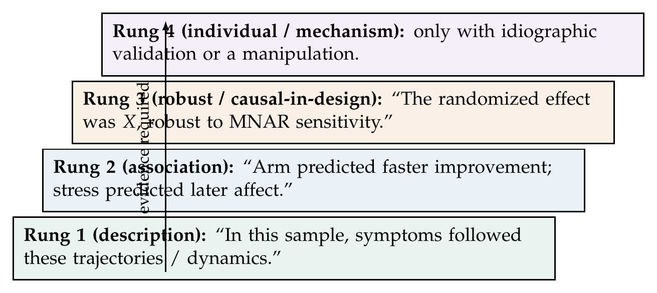
Note. The language a clinical longitudinal result has earned is fixed to the evidence that supports it. Description and association are available from most designs; a robust or causal-in-design claim requires randomization or a sensitivity analysis that bounds the missing-data threat; an individual-level or mechanistic claim requires idiographic validation or an experimental manipulation. Writing at the rung the evidence reaches, and no higher, is the discipline the three case studies share.
Table 33.6. Clinical Longitudinal Reporting Checklist
| Element | What to report |
|---|---|
| Estimand | The target of inference, including the dropout-handling strategy |
| Visualization | Trajectories and attrition before any model |
| Primary analysis | The pre-specified model and its arm/effect estimand |
| Missingness | The mechanism diagnosed and the sensitivity analyses |
| Heterogeneity | Exploratory subgroups labeled as such, unreified |
| Representations | For dynamics, the reconciliation of model, network, idiographic |
| Claims | Written at the rung of the ladder the evidence reaches |
Note. The checklist operationalizes the chapter’s spine. Its distinctive clinical additions to the general reporting standards of the book are the estimand’s dropout-handling strategy, the sensitivity analysis as a required element rather than an optional one, and the reconciliation of multiple representations where intensive longitudinal data invite selective reporting.
Common Pitfall • Four clinical over-reaches
Completer analyses. Analyzing only patients who finished discards the attrition that carries the bias; use all randomized patients under a named estimand, and probe the missingness. Reified responder classes. An exploratory mixture’s classes are a hypothesis, not discovered subtypes; do not build clinical decisions on them from one sample. Networks as mechanism. A symptom network’s edges are conditional associations; a clinical paper that reads them as causal levers has climbed past its evidence. Forecasting hype. A predictive model must beat the persistence baseline by a margin that survives grouped cross-validation and be calibrated; in-sample accuracy is not clinical readiness.
In Practice • Working with trial statisticians, and monitoring safety
Two practical matters recur in clinical work. Collaboration with trial statisticians is smoothed by a shared vocabulary: the estimand framework, the distinction between a hypothetical and a treatment-policy strategy, and the language of sensitivity analysis are the bridge, and a psychologist who brings the growth-model and joint-model machinery of this book to that conversation is a full partner rather than a supplicant. Second, high-frequency assessment of symptomatic patients demands a safety-monitoring protocol: momentary items that could surface acute risk, self-harm or suicidality, require a pre-specified response pathway, real-time review or escalation, that is designed before data collection and reported in the methods, because an assessment that could detect a crisis and does nothing about it is not ethically neutral.
In Practice • Ethics: momentary risk data and person-specific results
Clinical intensive longitudinal data raise ethical duties the analysis cannot outsource. Momentary suicidality or self-harm items generate data whose handling, storage, access, and response pathway must be specified in advance, because collecting such data creates a duty of care that does not end when the study does. Person-specific results carry their own risks: an idiographic model of one patient is identifiable in a way a group estimate is not, and reporting a striking individual coefficient, in a paper or back to the patient, risks both a privacy breach and an over-interpretation that the estimate’s uncertainty does not support. The discipline is to treat a person-specific finding as a clinical hypothesis held to the same standard of validation as any other, and to protect the patient’s data and privacy as carefully as the analysis protects its inferences.
Chapter Summary
The first applications chapter shows the book’s methods working together on clinical questions, where the decisions that matter are decisions about integration, sequencing, reconciliation, and reporting. Clinical questions route to methods by their estimand, efficacy trajectories to growth models, relapse to survival, dynamics to multilevel vector-autoregression and networks, delivery to micro-randomized trials, and the realities of symptom measurement, reactivity, nesting, and dropout shape every analysis, with the trials tradition adding the estimand framework in which the handling of dropout is part of the estimand itself. Case Study A takes a depression trial seriously: a growth model estimates the arm-by-time benefit, a mixed model translates it into remission, a hazard model diagnoses symptom-dependent dropout, and two sensitivity analyses, a tipping-point penalty that the benefit survives and a joint model that reproduces the naive estimate, converge to make the finding robust, the sensitivity analysis functioning as a first-class result rather than an appendix, with responder heterogeneity flagged only as guarded exploration. Case Study B studies symptom dynamics and insists that the multilevel model, the temporal network, and the idiographic portrait are one truth in three lenses, reconciled rather than reported selectively, with the network held to the claims-ladder discipline and the idiographic estimates shown against their shrunken counterparts so that neither the noisy individual number nor the regularized one is mistaken for the whole story. Case Study C separates the three activities digital mental health conflates: a micro-randomized trial estimates the causal excursion effect of a prompt and finds it wanes with habituation, a prediction model is judged against the persistence baseline by grouped cross-validation and calibration, and early-warning monitoring inherits the single-case sobriety of Chapter 32, each a different estimand needing a different design. The three case studies share a spine, visualize first, name the estimand first, analyze sensitivity always, and a claims ladder that writes each clinical conclusion at the rung its evidence has earned, together with the ethical duties, safety monitoring and person-specific privacy, that clinical data impose on the analyst.
aan het Rot, M., Hogenelst, K., & Schoevers, R. A. (2012). Mood disorders in everyday life: A systematic review of experience sampling and ecological momentary assessment studies. Clinical Psychology Review, 32(6), 510–523. https://doi.org/10.1016/j.cpr.2012.05.007
Boruvka, A., Almirall, D., Witkiewitz, K., & Murphy, S. A. (2018). Assessing time-varying causal effect moderation in mobile health. Journal of the American Statistical Association, 113(523), 1112–1121. https://doi.org/10.1080/01621459.2017.1305274
Bringmann, L. F., Vissers, N., Wichers, M., Geschwind, N., Kuppens, P., Peeters, F., Borsboom, D., & Tuerlinckx, F. (2013). A network approach to psychopathology: New insights into clinical longitudinal data. PLoS ONE, 8(4), Article e60188. https://doi.org/10.1371/journal.pone.0060188
Ebner-Priemer, U. W., & Trull, T. J. (2009). Ecological momentary assessment of mood disorders and mood dysregulation. Psychological Assessment, 21(4), 463–475. https://doi.org/10.1037/a0017075
Epskamp, S., van Borkulo, C. D., van der Veen, D. C., Servaas, M. N., Isvoranu, A.-M., Riese, H., & Cramer, A. O. J. (2018). Personalized network modeling in psychopathology: The importance of contemporaneous and temporal connections. Clinical Psychological Science, 6(3), 416–427. https://doi.org/10.1177/2167702617744325
Fisher, A. J., Reeves, J. W., Lawyer, G., Medaglia, J. D., & Rubel, J. A. (2017). Exploring the idiographic dynamics of mood and anxiety via network analysis. Journal of Abnormal Psychology, 126(8), 1044–1056. https://doi.org/10.1037/abn0000311
Gueorguieva, R., & Krystal, J. H. (2004). Move over ANOVA: Progress in analyzing repeated-measures data and its reflection in papers published in the Archives of General Psychiatry. Archives of General Psychiatry, 61(3), 310–317. https://doi.org/10.1001/archpsyc.61.3.310
Hamaker, E. L., & Wichers, M. (2017). No time like the present: Discovering the hidden dynamics in intensive longitudinal data. Current Directions in Psychological Science, 26(1), 10–15. https://doi.org/10.1177/0963721416666518
Heron, K. E., & Smyth, J. M. (2010). Ecological momentary interventions: Incorporating mobile technology into psychosocial and health behaviour treatments. British Journal of Health Psychology, 15(1), 1–39. https://doi.org/10.1348/135910709X466063
International Council for Harmonisation of Technical Requirements for Pharmaceuticals for Human Use. (2019). ICH harmonised guideline — Statistical principles for clinical trials: Addendum: Estimands and sensitivity analysis in clinical trials, E9(R1). ICH.
Kirtley, O. J., Lafit, G., Achterhof, R., Hiekkaranta, A. P., & Myin-Germeys, I. (2021). Making the black box transparent: A template and tutorial for registration of studies using experience-sampling methods. Advances in Methods and Practices in Psychological Science, 4(1), Article 2515245920924686. https://doi.org/10.1177/2515245920924686
Klasnja, P., Hekler, E. B., Shiffman, S., Boruvka, A., Almirall, D., Tewari, A., & Murphy, S. A. (2015). Microrandomized trials: An experimental design for developing just-in-time adaptive interventions. Health Psychology, 34(Suppl.), 1220–1228. https://doi.org/10.1037/hea0000305
Myin-Germeys, I., Kasanova, Z., Vaessen, T., Vachon, H., Kirtley, O., Viechtbauer, W., & Reininghaus, U. (2018). Experience sampling methodology in mental health research: New insights and technical developments. World Psychiatry, 17(2), 123–132. https://doi.org/10.1002/wps.20513
Myin-Germeys, I., Oorschot, M., Collip, D., Lataster, J., Delespaul, P., & van Os, J. (2009). Experience sampling research in psychopathology: Opening the black box of daily life. Psychological Medicine, 39(9), 1533–1547. https://doi.org/10.1017/S0033291708004947
Nahum-Shani, I., Smith, S. N., Spring, B. J., Collins, L. M., Witkiewitz, K., Tewari, A., & Murphy, S. A. (2018). Just-in-time adaptive interventions (JITAIs) in mobile health: Key components and design principles for ongoing health behavior support. Annals of Behavioral Medicine, 52(6), 446–462. https://doi.org/10.1007/s12160-016-9830-8
Shiffman, S., Stone, A. A., & Hufford, M. R. (2008). Ecological momentary assessment. Annual Review of Clinical Psychology, 4, 1–32. https://doi.org/10.1146/annurev.clinpsy.3.022806.091415
Trull, T. J., Solhan, M. B., Tragesser, S. L., Jahng, S., Wood, P. K., Piasecki, T. M., & Watson, D. (2008). Affective instability: Measuring a core feature of borderline personality disorder with ecological momentary assessment. Journal of Abnormal Psychology, 117(3), 647–661. https://doi.org/10.1037/a0012532