Chapter 34
Applications in Developmental and Educational Psychology
Longitudinal methodology was born in the study of development, and the hardest measurement problems in the whole field still live there. A child measured in third grade and again in eighth grade has changed on a scale that must itself be constructed before any change can be read, has aged while also advancing through grades while also belonging to a birth cohort whose world differed from the next, and has moved through classrooms and schools that leave their own imprint on the record. This chapter, the second of the applications part, works three developmental and educational questions end to end, and its throughline is that in this domain the measurement decisions precede and constrain the modeling decisions rather than following them. The first case study follows achievement across grades and does the thing that is rare in print: it carries a single dataset from the raw multi-wave merge through the adjudication of a time metric, the demonstration of measurement invariance, the interrogation of the vendor’s vertical scale, the growth model with its institutional nesting, the cohort-convergence test the accelerated design demands, and finally the policy translation, exposing at each step how a scaling choice made by a test publisher can reverse a conclusion about whether a gap is widening. The second studies developmental cascades and insists on the estimand discipline the published literature routinely forgets, separating the stable trait from the within-person transaction that a conventional cross-lagged panel model silently conflates. The third turns to cognitive aging and to the measurement-burst design that samples a slow process at a fast timescale, testing the aging literature’s signature hypothesis that within-person variability rises before the mean declines, and doing so with the sobriety that a short series and a selective attrition demand. The unifying lesson is Wohlwill’s: describing change is not the same as explaining development, and the distance between them is exactly the space this chapter tries to make visible.
Learning Objectives
After working through this chapter, you should be able to: (1) choose a developmental time metric (age, grade, wave, or a maturational clock) by the estimand it serves and defend the choice; (2) analyze an accelerated cohort-sequential design and test its convergence assumption rather than presuming it; (3) integrate institutional nesting, including the cross-classification created when children change schools, into a growth model; (4) interrogate a vertical scale at consumer depth, recognizing that a growth conclusion can depend on the ruler as much as on the child; (5) estimate developmental cascades with the between-person and within-person components separated, and resist the cross-lagged-panel habit; (6) analyze measurement-burst data for change in variability and change in dynamics, not only change in level; and (7) report developmental and educational findings, including months-of-learning translations, with their assumptions stated rather than hidden.
34.1 The Developmental-Educational Terrain
Questions about development and schooling fall into a small number of families, and naming the family is the first analytic act because it determines both the estimand and the chapter that supplies the tool. Whether a capacity changes on average, and along what shape, is a question about normative change, answered by the growth-curve models of Chapters 13 and 14. Whether children differ in their change, and what predicts the difference, is a question about individual differences in change, answered by the random effects of those same models read at the person level. Whether one developing system drives another, so that reading pulls up later mathematics or engagement pulls up later achievement, is a transactional or cascade question, answered by the panel-model family of Chapters 20 and 21. Whether the classroom, the teacher, or the school leaves a mark is an institutional-effects question, answered by the multilevel models of Chapters 13 and 14 extended to the nesting that education always imposes. And whether the fluctuation itself is the phenomenon, as in the inconsistency that heralds cognitive decline, is a variability-as-construct question, answered by the intensive-longitudinal and dynamic tools of Chapters 7, 16, and 25. Figure 34.1 draws the routing and Table 34.1 sets it out with estimands and exemplar literatures.
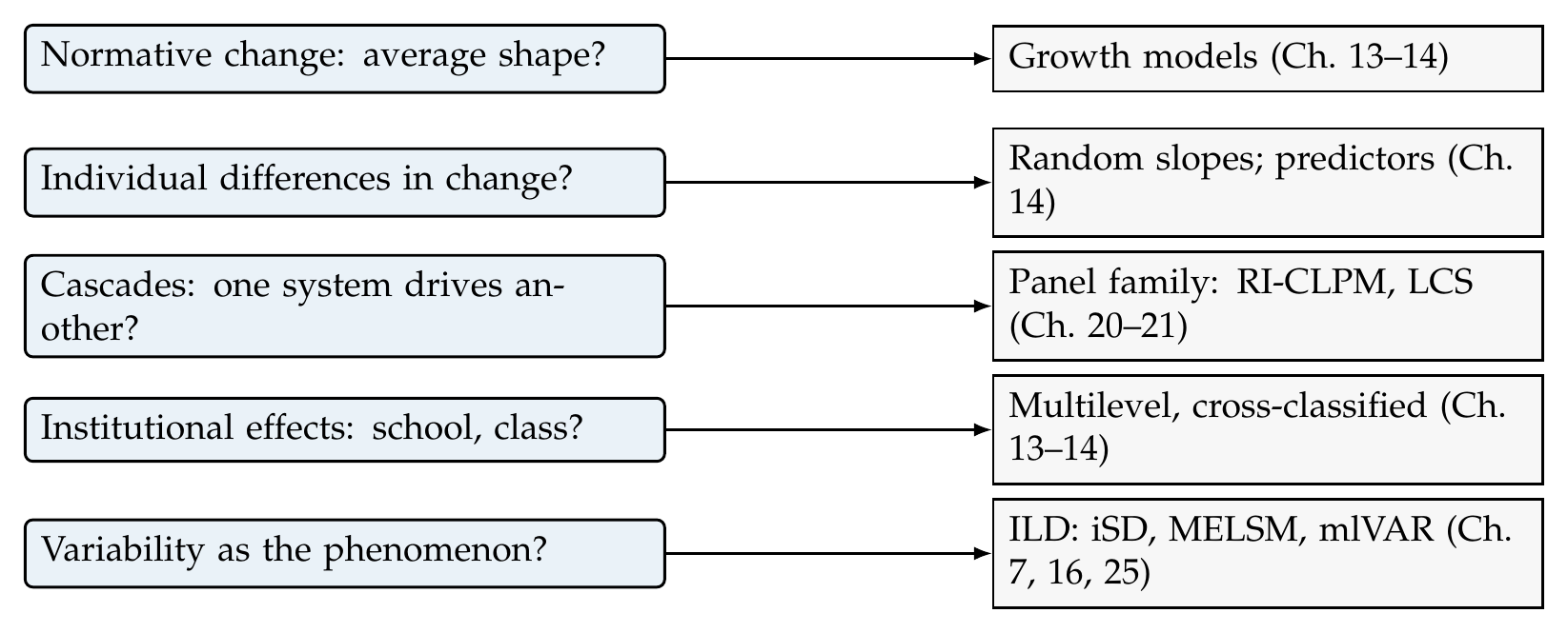
Note. Each family of question routes to the part of the book that answers it, estimand first. A developmental study usually asks several at once, and the analytic craft is to sequence the corresponding analyses so that each informs the next, which is what the three case studies of this chapter demonstrate.
Table 34.1. Question Taxonomy, Estimands, Chapters, and Domain Exemplars
| Question family | Estimand | Chapters | Exemplar |
|---|---|---|---|
| Normative change | Mean trajectory shape | 13–14 | McArdle & Epstein (1987) |
| Individual differences | Variance of change; predictors | 14 | Duncan & Duncan (2009) |
| Cascades | Within-person cross-lag | 20–21 | Masten & Cicchetti (2010) |
| Institutional effects | Level-2/3 variance | 13–14 | Raudenbush & Bryk (2002) |
| Variability as construct | Change in within-person SD | 7, 16, 25 | Ram & Gerstorf (2009) |
Note. The estimand column is the discipline. A single developmental dataset routinely supports several of these targets, and the analyst’s task is to name the one in play before selecting a model, because the same data answer different questions with different specifications.
Behind all of these sits the domain’s defining difficulty, which is that the thing being measured does not hold still while it is measured. A construct can change its behavioral expression across development even as it remains the same construct, the heterotypic continuity of Chapter 3, so that fear looks like separation distress in a toddler and like social avoidance in an adolescent, and a single indicator set cannot serve both. Even when the expression is stable, the scale on which scores are reported must be shown to mean the same thing at each age before a difference between ages can be interpreted as change rather than as measurement drift, which is the invariance problem of Chapter 18 recast across the developmental range. And in achievement testing specifically, the scores that a district hands the analyst arrive already transformed onto a vertical scale whose construction embeds assumptions that the analyst did not make and often cannot see, a problem this chapter treats at length because it is where measurement and modeling collide most consequentially. The three clocks compound the difficulty: a child’s age, grade, and birth cohort advance together in ordinary designs and can only be separated by designs that deliberately break their collinearity, which is the age-period-cohort predicament of Chapter 2 wearing developmental clothes, with the added subtlety that in schooling data the school-entry cutoff acts as a regression-discontinuity boundary that a careful analyst can exploit.
The data themselves arrive with their own realities. Consent in developmental research is a chain rather than an event, with parental consent renewed and child assent added as the child matures, and attrition that is anything but random because the families who leave a study differ systematically from those who stay. School records must be linked across years and across administrative systems that were not built to be linked, and children move, so that the tidy nesting of pupils within one school gives way to the cross-classification of pupils within the several schools they attend over time. Large-scale assessments such as the national longitudinal studies buy representativeness and vertical scaling at the cost of thin measurement occasions, while laboratory longitudinal studies buy dense, well-characterized measurement at the cost of small and selected samples, and the design trade-off between them is not resolvable in the abstract but only against a specific estimand. Figure 34.2 shows the three-clocks problem in the concrete, plotting the same simulated achievement records on the wave, grade, and age axes and letting the eye see how differently the cohorts align depending on which clock is chosen.
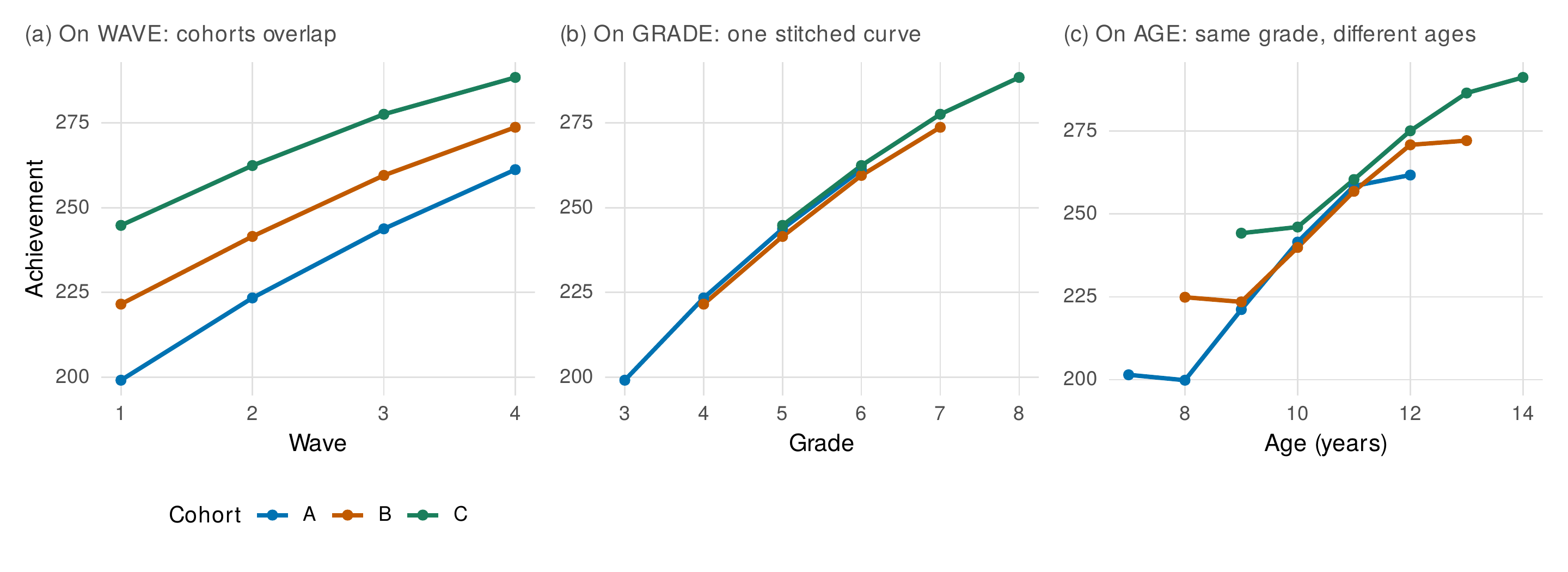
Note. Cohort means from the achieve_accel accelerated design (three cohorts entering grades 3, 4, and 5). On the wave axis (a) the cohorts appear as parallel curves and the grade span they jointly cover is invisible. On the grade axis (b) the overlapping segments stitch into a single accelerated growth curve spanning grades 3 to 8, which is the alignment the design was built to permit. On the age axis (c) children of the same grade but different ages are spread out and the segments no longer coincide, because in these data growth is driven by schooling rather than by age. The figure is the argument for choosing the clock by the estimand.
34.2 Case Study A: Achievement Growth Across Grades
The first case study takes an accelerated, school-nested achievement dataset and carries it through the full measurement-to-policy chain, because that chain is where the domain’s characteristic decisions are made and because seeing them made in sequence is worth more than any one of them treated in isolation. The data are the simulated achieve_accel records: 1,200 children in 30 schools, measured across four annual waves in three overlapping grade cohorts that jointly span grades 3 through 8, with a known decelerating growth process on a latent ability metric, planted effects of socioeconomic status on both the level and the rate of growth, entry-age variation that decouples age from grade, and a fraction of children who change schools between waves. Because the truth is known by construction, every estimate below can be audited against it, which is the pedagogical purpose of a simulated example and the reason the numbers are reported to a precision that real data would not warrant.
34.2.1 Adjudicating the Time Metric
The first substantive decision is which clock to model, and it is a decision about the estimand, not about model fit. If the question concerns the effect of schooling, grade is the natural metric because grade indexes exposure to instruction; if the question concerns maturation, age is the natural metric; and the two diverge exactly to the degree that children of the same grade differ in age, through delayed school entry, redshirting, or retention. Fitting the same decelerating growth model to the achievement scores on the grade metric recovers a grade-3 gain of 25.1 score points per grade against a planted truth of 25 and a negative quadratic of \(-1.53\) that reproduces the deceleration, whereas fitting on the age metric attenuates the linear gain to 23.7 points per year and, more tellingly, inflates the estimated between-child variability in the growth rate, because aligning a schooling-driven process on age spreads the schooling signal across the ages at which children happen to sit in each grade. In these data the divergence is modest because the within-grade age spread is modest, a within-grade age standard deviation of about half a year, and the honest conclusion is not that one metric is right and the other wrong but that the grade metric is the sharper ruler for a schooling-driven estimand and that the divergence between the two would grow with the age heterogeneity that retention and delayed entry introduce. Table 34.2 records the decision as a reviewer would want to see it recorded, with the estimand, the metric chosen, the alternative examined, and the reconciliation.
Table 34.2. Time-Metric Adjudication: The Case A Decision Log
| Element | Grade metric | Age metric |
|---|---|---|
| Estimand served | Effect of schooling (instructional exposure) | Effect of maturation |
| Linear gain | 25.1 pts/grade (truth 25) | 23.7 pts/year (attenuated) |
| Shape | Decelerating (quadratic \(-1.53\)) | Decelerating, flatter |
| Slope heterogeneity | Smaller (aligned signal) | Larger (misaligned signal) |
| Verdict | Preferred for a schooling estimand | Preferred for a maturational estimand |
Note. Both metrics were fit; the choice follows the estimand, not the fit statistic. The divergence is modest here because within-grade age variation is modest, and would sharpen with retention or delayed entry. Reporting both, and reconciling them, is the defensible practice.
34.2.2 The Measurement Layer: Invariance, Then the Ruler
Before any score difference across grades can be read as growth, two distinct measurement questions must be answered, and confusing them is a common error. The first is whether the measure functions the same way at each grade, which is the longitudinal invariance question. Fitting a longitudinal factor model to the six-indicator achievement measure across the four waves of the youngest cohort and imposing invariance in sequence, the configural, metric, and scalar models all fit essentially perfectly, with comparative fit indices at 1.000 and changes in comparative fit of 0.000 at both the metric and scalar steps, which is what invariance planted by construction should look like and which licenses the interpretation of the composite as measuring one construct on one scale across the grades. The second question is entirely separate and concerns the interval properties of the reported scale itself, and here the achievement literature hides a decision that most consumers never examine.
Foundations Box • The vertical-linking sketch
A vertical scale places scores from different grades on one continuum so that a third-grade and an eighth-grade score can be compared and their difference called growth. The construction rests on common items administered to adjacent grades: an item answered by both fourth and fifth graders links the two grade-level calibrations, and a chain of such links, calibrated through an item-response model, propagates a single scale across the whole range. The procedure is principled, but it is not unique. The choice of item-response model, the linking design, the population used to anchor the scale, and the method of placing successive grades all leave fingerprints on the resulting interval spacing, and different defensible choices produce scales that agree on the ordering of children while disagreeing on the size of a gain. The consumer’s obligation is not to build the scale but to ask the vendor which choices were made and to test whether the study’s conclusions survive plausible alternatives. Kolen and Brennan (2014) is the authority; the point for the analyst is that a vertical scale is a construction, not a measurement, and growth is read through it.
The consequence is the chapter’s set piece, which Figure 34.3 makes concrete. Taking the one latent growth process and passing it through three monotone rescalings, each a plausible vendor scale that preserves the ordering of every child at every grade, the shape of average growth changes qualitatively: on the interval-faithful linear scale the growth decelerates, with a negative quadratic of \(-0.036\) in standardized units; on a convex scale that expands the upper range the same growth appears to accelerate, the quadratic flipping sign to \(+0.034\); and on a concave scale that compresses the upper range the growth appears to plateau, the deceleration deepening to \(-0.067\). The reversal is not a numerical curiosity but a substantive one, because the sign of the quadratic is exactly the quantity a policy analyst would cite to argue that learning slows or accelerates through the middle grades. Worse for equity research, the estimate of whether the socioeconomic gap widens with grade swings sevenfold across the three scales, from a standardized socioeconomic-by-grade interaction of 0.028 on the concave scale, through 0.088 on the linear scale, to 0.192 on the convex scale, so that the same children generate a story of a barely-widening gap or a rapidly-widening one depending entirely on a scaling choice made by a test publisher. Table 34.3 lays out the assumptions, the construction, and the sensitivity findings.
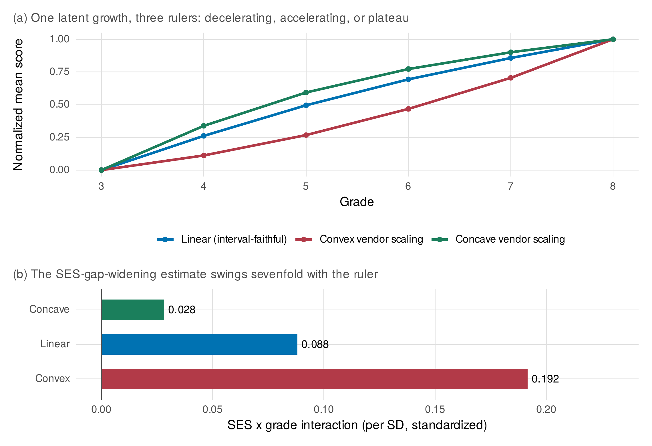
Note. Panel (a) shows the population mean of the same simulated latent growth after three monotone rescalings, each normalized to its own range so that only shape is compared: the convex vendor scale bends the curve below the diagonal (apparent acceleration), the concave scale above it (apparent plateau), with the interval-faithful linear scale between. Panel (b) shows the socioeconomic-by-grade interaction, the estimate of gap widening, under each scaling; it swings from 0.028 to 0.192 although no child’s rank changed at any grade. The scale, not the child, drives the conclusion.
Table 34.3. Vertical Scaling: Assumptions, Construction, and Sensitivity
| Scaling | What it assumes | Effect on the conclusion |
|---|---|---|
| Linear (interval-faithful) | Equal-interval latent metric preserved | Decelerating growth; gap widening 0.088 |
| Convex (upper expansion) | Later gains count for more | Apparent acceleration; gap widening 0.192 |
| Concave (upper compression) | Later gains count for less | Apparent plateau; gap widening 0.028 |
Note. All three scales are monotone transforms of one latent growth process and preserve every child’s rank at every grade. The interval-level conclusions, the sign of the deceleration and the magnitude of gap widening, are not preserved. Sensitivity to the scaling should be reported whenever a growth claim is interval in nature.
Common Pitfall • Grade-equivalents and interval claims
The most common scaling error in educational research is to treat a grade-equivalent score, or an unexamined vendor scale score, as if it carried interval meaning, and then to compute and compare gains as though a point at the bottom of the range equaled a point at the top. Grade-equivalent scores are especially treacherous because they are defined by median performance and behave non-linearly, so that a fixed number of grade-equivalent units means different amounts of learning at different points. The remedy is not to abandon the scores but to state the scale’s provenance, to prefer scales with a defensible interval justification for interval claims, and to run the growth conclusion through alternative scalings as a sensitivity analysis, exactly as Figure 34.3 does. A gap-widening finding that survives only on one vendor’s scale is a finding about the vendor, not about the children.
34.2.3 Growth With Institutional Nesting
Children are nested in schools, and in a longitudinal design the nesting is not clean because children move. In these data 180 of the 1,200 children change schools at some wave, and the question is whether to model each child’s home school, ignoring the move, or to model the current school at each occasion, which cross-classifies children with the several schools they attend. Fitting the growth model both ways, the single-membership specification that ignores mobility attributes a between-school variance of 123.4 and a residual standard deviation of 7.21, while the cross-classified specification that credits each occasion to its actual school reduces the between-school variance to 88.9 and the residual to 7.00, because the single-membership model forces a mover’s post-move occasions to load on the wrong school and absorbs the misfit as inflated variance. The lesson generalizes: mobility is not a nuisance to be dropped by listwise deletion of movers, which would select on exactly the disadvantage that mobility marks, but a structural feature to be modeled by cross-classification. Figure 34.4 diagrams the structure.
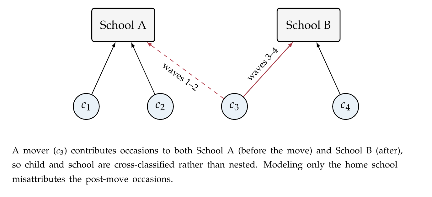
Note. Most children attend one school, but a mover’s occasions belong to different schools at different waves, crossing the child and school groupings. A cross-classified random-effects model credits each occasion to its actual school; a single-membership model that uses only the home school inflates the between-school variance, here from 88.9 to 123.4, by forcing post-move occasions onto the wrong unit.
34.2.4 The Accelerated Design’s Convergence Test
An accelerated design pools cohorts that each cover part of the grade range, aligning them on grade to reconstruct a span no single cohort was followed across. The reconstruction is valid only if the cohorts share the same growth process at the grades they have in common, an assumption of cohort convergence that the design makes testable rather than merely assumes. Adding cohort main effects and cohort-by-grade interactions to the growth model and comparing by likelihood-ratio test yields a non-significant result, \(p = .94\), so the convergence assumption holds in these data, as it was planted to. The point of method is that the assumption is not to be presumed on faith but examined, because a secular trend in achievement, in curriculum, or in technology exposure across cohorts is the norm rather than the exception in real educational data, and a failed convergence test is not a nuisance but a finding about cohort effects that the accelerated design is uniquely positioned to detect.
34.2.5 Predictors, Flexibility, and the Policy Translation
With the growth model established, the predictors of the trajectory can be read. Socioeconomic status raises the grade-3 level by 12.2 points per standard deviation and the growth rate by 3.74 points per grade per standard deviation, the latter the widening-gap effect that survived the scaling scrutiny above on the interval-faithful scale. A flexibility check guards against having imposed the decelerating quadratic where the data wanted something else: a generalized additive model with a smooth of grade returns an effective degrees of freedom of 3.8, and the information criterion does not favor the smooth over the parametric quadratic, the difference in Akaike’s criterion being 2.5 in the quadratic’s favor, so the parsimonious decelerating curve is adequate and the nonlinearity is genuinely quadratic rather than something the polynomial missed. Figure 34.5 assembles the case: the stitched decelerating growth, the between-school variation, and the widening socioeconomic gap.
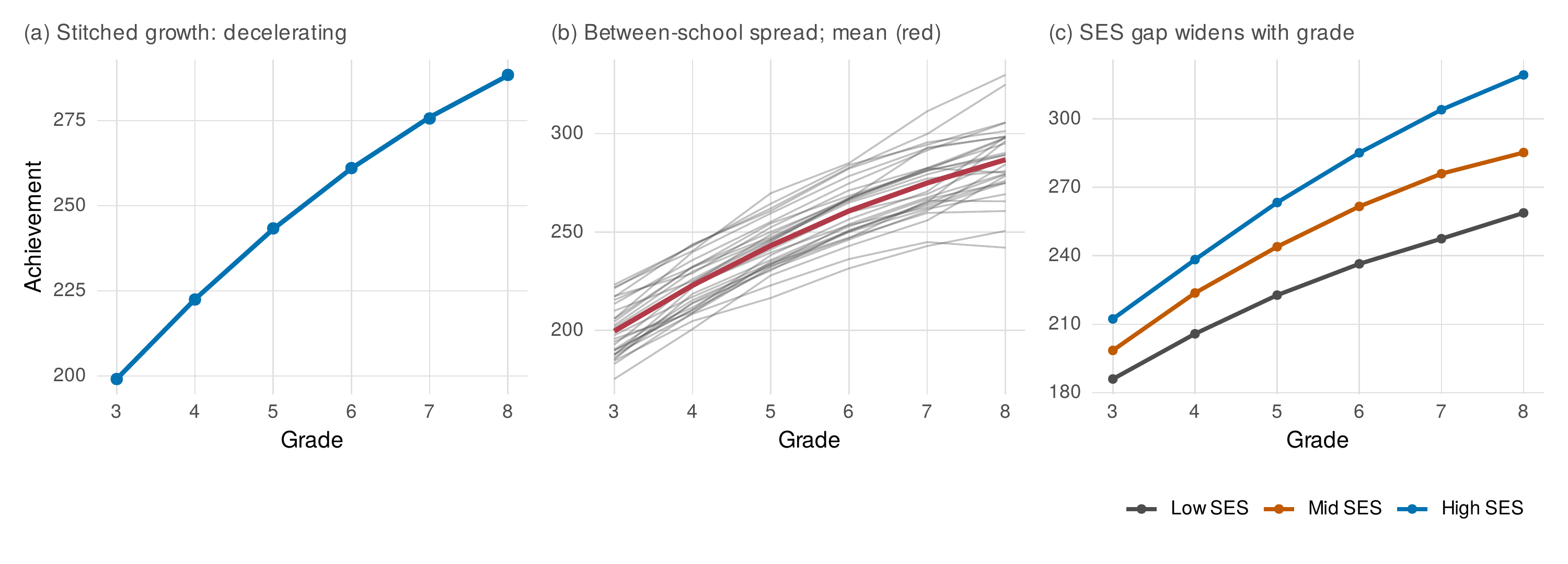
Note. Panel (a) shows the cohort-stitched mean achievement with its fitted decelerating quadratic. Panel (b) shows the 30 school-mean trajectories (grey) around the grand mean (red), the institutional variation the multilevel model partitions. Panel (c) shows mean achievement by grade within socioeconomic tertiles, the gap widening across grades on the interval-faithful scale, a conclusion the reader now knows to hold conditional on that scale.
The final step is the translation that policy audiences ask for, the expression of an effect in months of learning, and it must be done with its hazard stated. Dividing the socioeconomic gap at grade 3, 12.2 points, by the average annual gain of about 25 points and multiplying by the nine months of a school year renders the gap as roughly 4.4 months of learning, and the annual widening of 3.74 points as about 1.3 additional months per year. The translation is communicatively powerful and analytically fragile, because it inherits every assumption of the scale, so that the same gap expressed on the convex vendor scale would translate to a different and larger number of months, and because it divides by an average gain that is itself decelerating and therefore not constant across the range being described. A months-of-learning figure should therefore never be reported without the scale it rests on and the caveat that it is a communicative device rather than a measurement. Table 34.4 collects the reporting obligations, and the practice box addresses the realities of the district data such a study runs on.
Table 34.4. Education and Development Reporting Checklist
| Element | What to report |
|---|---|
| Time metric | The clock modeled, the estimand it serves, and the reconciliation with the alternative |
| Invariance | The invariance level established and the change-in-fit evidence for it |
| Vertical scale | The scale’s provenance and a sensitivity of the growth conclusion to alternatives |
| Nesting and mobility | The nesting structure, including cross-classification for movers |
| Cohort convergence | The convergence test, not an assumption |
| Months-of-learning | The scale it rests on and its status as a communicative device |
Note. The checklist encodes the chapter’s claim that in this domain the measurement decisions are reportable results, not preliminaries. A growth finding whose scale, metric, and nesting are unstated is not yet interpretable.
In Practice • In Practice: working with district and archival data
District achievement data arrive linked across years by administrative identifiers that were built for accounting rather than research, and the analyst’s first task is a documented merge, per the data-provenance discipline of Chapter 5, that reconciles duplicate records, mid-year transfers, and identifier changes before any model is fit. Privacy regimes such as the family-educational-records protections in the United States constrain what may be linked and released, and a defensible study states its data-use agreement and its de-identification rather than leaving them implicit. Much developmental and educational work is secondary analysis of archival longitudinal studies, and although the data predate the analyst, the analysis plan does not: the estimand, the model, the invariance and scaling checks, and the sensitivity analyses can and should be preregistered even when the data are already collected, because preregistration disciplines the analyst, not the data.
34.3 Case Study B: Developmental Cascades
The second case study turns to transaction, the developmental idea that systems shape each other over time, so that a child’s verbal ability lifts later performance ability or engagement lifts later achievement, and it insists on the estimand discipline that the cascade literature has too often neglected. The data are the simulated wisc records, a bivariate verbal-and-performance ability design measured across four annual waves in 900 children, built with a known cross-lagged process in which stable person traits are correlated across the two domains and the within-person transactions are directional, verbal driving later performance far more than the reverse, with socioeconomic status moderating the strength of that transaction. The construction lets the analysis be audited and, more importantly, lets the consequences of the wrong model be shown.
34.3.1 Separating the Trait From the Transaction
The estimand of a cascade claim is a within-person effect: the question is whether a child who is higher on verbal ability than that child usually is goes on to be higher on performance ability than that child usually is, which is a statement about within-person deviations from a person’s own trajectory. The conventional cross-lagged panel model does not estimate this, because it regresses observed scores on observed scores without separating the stable between-person differences, so that its cross-lags conflate the within-person transaction with the between-person correlation of stable traits, and the random-intercept cross-lagged panel model of Chapter 21 exists precisely to effect the separation. Fitting both to the same data, the random-intercept model recovers the planted directional cascade, a verbal-to-performance within-person path of 0.202 against a truth of 0.25, comfortably within its confidence interval, and a near-zero performance-to-verbal path of 0.058 against a truth of 0.05, with the correlated stable traits captured by a between-person covariance of 0.53, whereas the conventional model without random intercepts compresses the asymmetry, pulling the verbal-to-performance path down to 0.154 and inflating the performance-to-verbal path to 0.093, so that the five-to-one directional ratio in the truth collapses to less than two-to-one and the cascade’s direction is muddied. Figure 34.6 shows the contrast and the moderation, and Table 34.5 sets the estimates against the truth.
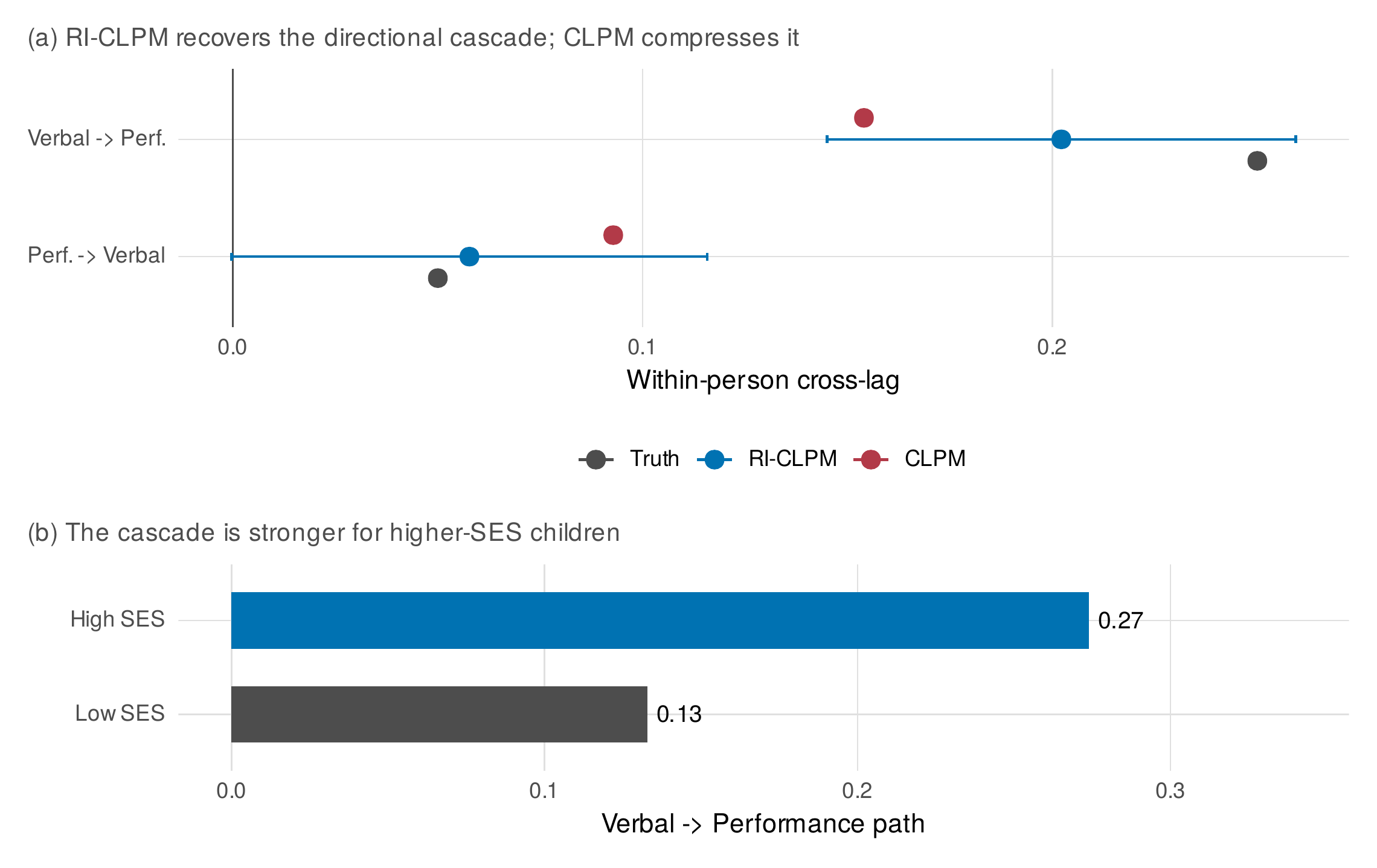
Note. Panel (a) plots the within-person cross-lags. The random-intercept cross-lagged panel model (blue) recovers the planted directional cascade, near the truth (grey), with the strong verbal-to-performance path and the near-zero reverse path; the conventional cross-lagged panel model (red), lacking random intercepts, compresses the asymmetry by absorbing the correlated stable traits into the lags. Panel (b) shows the verbal-to-performance path estimated separately by socioeconomic group: the cascade is stronger for higher-status children, the planted moderation.
Table 34.5. Cascade Model Family: Estimates Against the Truth
| Quantity | Truth | RI-CLPM | CLPM |
|---|---|---|---|
| Verbal \(\rightarrow\) performance | 0.25 | 0.202 | 0.154 |
| Performance \(\rightarrow\) verbal | 0.05 | 0.058 | 0.093 |
| Trait covariance / correlation | 0.50 | 0.53 | (absorbed) |
| Directional ratio | 5.0 | 3.5 | 1.7 |
Note. The random-intercept model (RI-CLPM) recovers the within-person directional cascade; the conventional model (CLPM) conflates the correlated stable traits with the lagged dynamics and compresses the directional ratio. The published habit of reporting CLPM cross-lags as evidence of a cascade is the target of this comparison.
A bivariate latent change score model, the coupled dual-change-score specification of Chapter 20, offers a secondary view on a different parameterization, in which change in one domain is regressed on the prior level of the other. It agrees with the random-intercept model on the direction of the cascade, returning a verbal-to-performance coupling of 0.099 against a performance-to-verbal coupling of 0.078, but the asymmetry is milder on this metric and the model’s parameter covariance is near-singular here, so it is read as a corroboration of direction rather than as an independent magnitude, and the reconciliation of the two model families follows the framework of Usami and colleagues rather than a contest between them. The moderation is estimated by freeing the verbal-to-performance path across a median split on socioeconomic status, which recovers a stronger cascade for higher-status children, 0.274 against 0.133 for lower-status children, the planted interaction that would, in a substantive study, invite a discussion of the resources that let one developing capacity leverage another.
34.3.2 The Interval Behind the Lag
A cross-lagged effect estimated on annual waves is silent about the interval it rests on, and the silence is a trap. A within-person lagged effect is not a fixed quantity but a function of the time between measurements, rising from zero at zero lag, peaking at some interval characteristic of the process, and decaying thereafter, exactly the continuous-time logic of Chapter 27, so that an annual-wave cascade estimate samples a single point on an underlying curve and a study with semiannual or biennial waves would report a different number for the same process. Figure 34.7 draws the point conceptually. The implication for developmental cascade research is not that annual designs are wrong but that their estimates are interval-specific, that comparisons across studies with different spacings are comparisons of different points on the curve rather than of the same effect, and that a continuous-time formulation is the principled remedy when the interval structure varies.
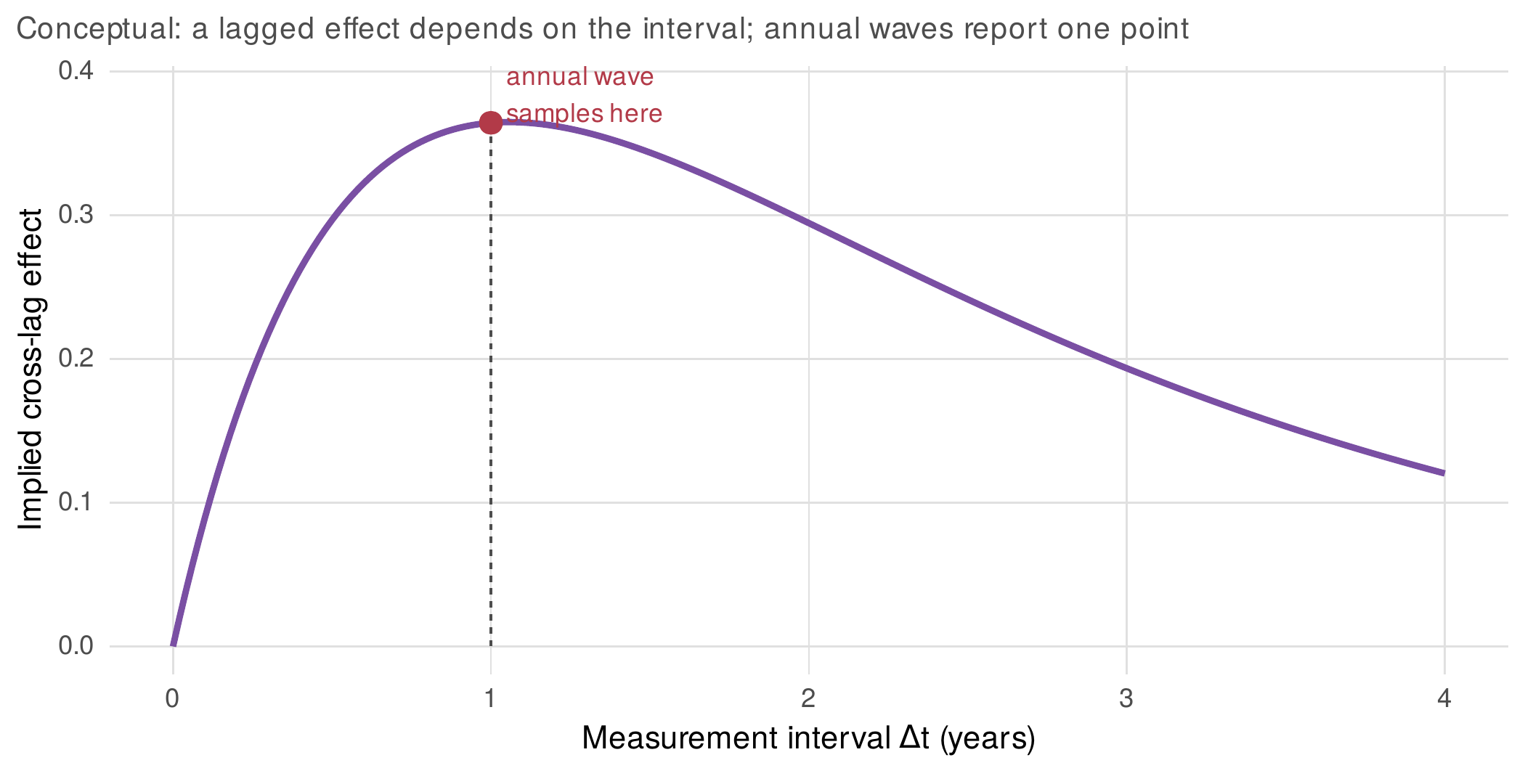
Note. Conceptual illustration. A within-person cross-lagged effect varies with the interval between measurements, here rising, peaking near a one-year lag, and decaying. An annual-wave design reports the single marked point; a design with different spacing would report a different value for the same underlying process. Cross-study comparisons of cross-lags implicitly assume a common interval that is rarely met, which the continuous-time models of Chapter 27 address directly.
Common Pitfall • Cascades from cross-lagged-panel models alone
The published developmental-cascade literature is dense with claims resting on a conventional cross-lagged panel model, in which any pair of significant cross-lags is read as evidence that one system drives another. The problem is that such cross-lags conflate stable between-person differences with within-person transactions, so that two constructs that are merely correlated in their stable levels will produce significant cross-lags in the absence of any transaction at all. A cascade claim requires a model that separates the person’s stable level from the person’s fluctuations around it, a random-intercept cross-lagged panel model or a latent change score model, and a study that reports only conventional cross-lags has not yet provided evidence for a cascade in the within-person sense the theory intends. The correction is not new, but its uptake is incomplete, and a reviewer is entitled to ask for it.
34.4 Case Study C: Variability and Bursts in Cognitive Aging
The third case study turns to the other end of the lifespan and to a design that samples a slow process at a fast timescale, the measurement-burst design, in which short periods of dense daily measurement are repeated at long intervals so that fast within-person dynamics can be tracked as they themselves change across the slow developmental time of aging. The data are the simulated burst_aging records: 250 older adults measured in three bursts of daily testing spread across three years, with processing speed and memory lapses recorded daily within each burst and a cognitive composite recorded once per burst. The design is built to carry the aging literature’s signature hypothesis, that within-person inconsistency rises before the mean declines, and to make the two hazards of testing that hypothesis visible, the short series that biases the dynamics and the selective attrition that biases the mean.
34.4.1 Three Analytic Layers
A burst design supports three distinct estimands at three timescales, and Table 34.6 sets them out. Within a burst, the daily data support a within-person mean, a within-person variability, and a within-person autocorrelation, the last two being the inconsistency and the sluggishness that the aging literature treats as constructs in their own right. Between bursts, the change in each of these person-and-burst quantities across the slow aging time is the developmental estimand, so that the question is not only whether the mean declines but whether the variability grows and whether the dynamics slow. And at the wave level, the cognitive composite provides the anchoring outcome against which the fast-timescale indicators are validated. Figure 34.8 shows the raw multi-timescale structure for a single participant, whose burst means drift upward, toward slower responding, while the day-to-day spread widens across the three bursts.
Table 34.6. Burst-Analytic Layers: Timescales, Estimands, and Models
| Layer | Estimand | Model |
|---|---|---|
| Within burst | Mean, within-person SD (iSD), autocorrelation | Descriptive per person-burst; AR(1) |
| Between bursts | Change in mean, iSD, and autocorrelation across aging | Growth of the person-burst quantities |
| Wave level | Cognitive level and its decline | Composite trajectory; attrition model |
Note. One burst dataset yields estimands at three timescales. The developmental questions live at the between-burst layer, where change in variability and change in dynamics, not only change in level, are the phenomena of interest.
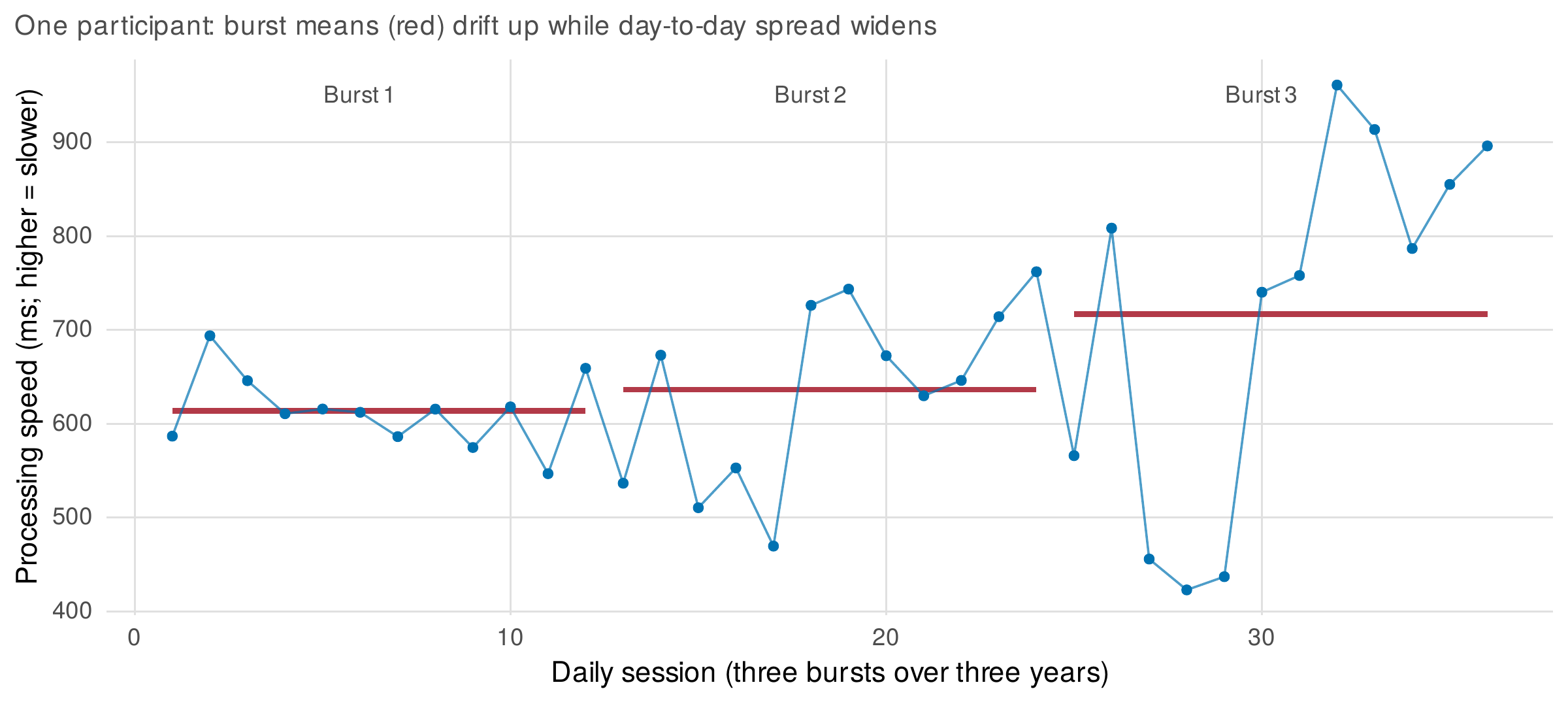
Note. Daily processing-speed measurements for one older adult across three bursts spanning three years, with burst means in red. The mean drifts upward, toward slower responding, and the day-to-day spread widens markedly by the third burst. The figure shows why a burst design is needed: the change in variability is invisible to a design that measures once per wave, because it lives at the within-burst timescale.
34.4.2 Does Variability Precede Decline?
The aging literature’s signature hypothesis is that within-person inconsistency is an early indicator, rising before the mean itself declines, and the burst structure lets it be tested directly. Across the three bursts the population mean processing speed is essentially flat from the first burst to the second, 650 then 656 milliseconds, before rising to 687 at the third, whereas the within-person variability rises already at the second burst, a median inconsistency of 53, 76, and 100 milliseconds across the three, so that the variability moves a full burst ahead of the mean. Figure 34.9 shows the lead. The person-level version of the claim, that a given adult’s burst-two variability forecasts that adult’s subsequent decline, is supported but modest: regressing the change in mean speed from the second to the third burst on burst-two inconsistency among the completers yields a positive coefficient of 0.51, standard error 0.23, \(p = .026\), a correlation of about 0.18, which is real but small and exactly the magnitude that should be reported without inflation. The sobriety is deliberate and echoes the caution of Chapter 32 against reading too much into early-warning indicators: variability as a leading marker is a genuine and useful phenomenon, and it is not a deterministic predictor of any individual’s trajectory.
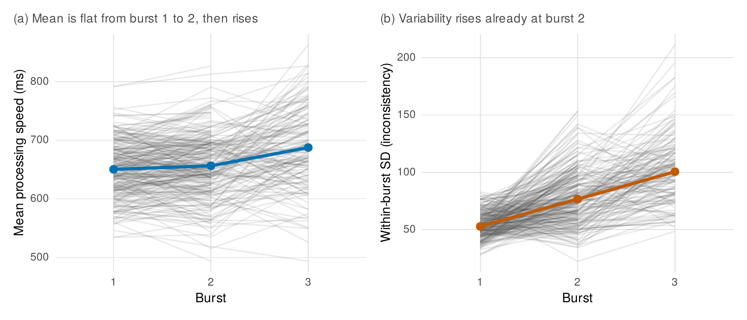
Note. Person trajectories (grey) and the population summary (coloured) across the three bursts. Panel (a): the mean processing speed is flat from burst 1 to burst 2, then rises at burst 3. Panel (b): the within-burst variability rises already at burst 2, a full burst ahead of the mean. The lead of variability over level is the aging literature’s signature hypothesis, here recovered from data built to contain it, with the person-level version modest in size.
34.4.3 Changing Dynamics and Selective Attrition
Beyond level and variability, the dynamics themselves change: the within-burst autocorrelation of processing speed, the sluggishness with which a slow response is followed by another slow response, rises across the bursts, and estimating it by a multilevel autoregression within each burst recovers the increase, autocorrelations of 0.12, 0.20, and 0.28 across the three bursts. The estimates are biased downward relative to the planted values of 0.25, 0.36, and 0.47 by the short twelve-day series, the small-sample dynamic-panel bias familiar from Chapters 24 and 25, but the increase across bursts, the dynamics-change signal that is the developmental estimand, is recovered clearly and is the quantity the study cares about. The second hazard is attrition, and here it is informative rather than benign: the adults who leave before the third burst are the more variable and the faster-declining, so that the third-burst sample is a survivor sample and its naive mean understates the population decline. The naive completer mean at the third burst is 687 milliseconds against a population truth of 705, and reweighting the completers by the inverse of their modeled probability of staying, an inverse-probability-of-attrition weighting that credits the departed high-risk cases, moves the estimate to 696, recovering roughly half of the survivor bias, with the residual gap a reminder that the correction can only adjust on what was measured. The full remedy, when the outcome and the dropout share unmeasured causes, is the joint modeling of the longitudinal process and the attrition process introduced in Chapter 29, and the burst design’s selective mortality is the developmental instance of that general problem.
In Practice • Ethics: assent across waves and incidental findings
Developmental research consents children over years during which their capacity to assent grows, and the ethical obligation is continuous rather than discharged at enrollment: assent is renewed as the child matures, and a design states how it re-consents participants who cross developmental thresholds during the study. Longitudinal cognitive and educational measurement can surface incidental findings, an unexpected decline in an older adult, a learning difficulty in a child, and a study specifies in advance what will be returned to participants, families, or schools and through what channel, because the measurement-burst intimacy of daily testing and the institutional setting of school data both raise the likelihood that something actionable will be seen. The principle is that the duty of care extends across the whole span of a longitudinal relationship, not only its first occasion.
34.5 Domain Synthesis
The three case studies share a structure, and Figure 34.10 abstracts it into a claims ladder that ascends from what longitudinal data most securely support to what they most tenuously support. At the bottom sits description, the documentation that a mean changes in a certain shape, which growth models deliver with high credibility once the measurement is sound. Above it sits the characterization of individual differences in change and their correlates, secure to the degree that the measurement is invariant and the scale interval-faithful. Higher still sits the within-person transaction, the cascade, which requires the between-person and within-person components to be separated and which annual designs estimate only at a fixed interval. And at the top sits the developmental explanation, the claim that one thing causes the developmental emergence of another, which longitudinal description constrains but does not establish, because as Wohlwill argued and Baltes and Nesselroade insisted, the description of change is a different achievement from the explanation of development, and the gap between them is bridged by theory and design, not by a longer panel alone.
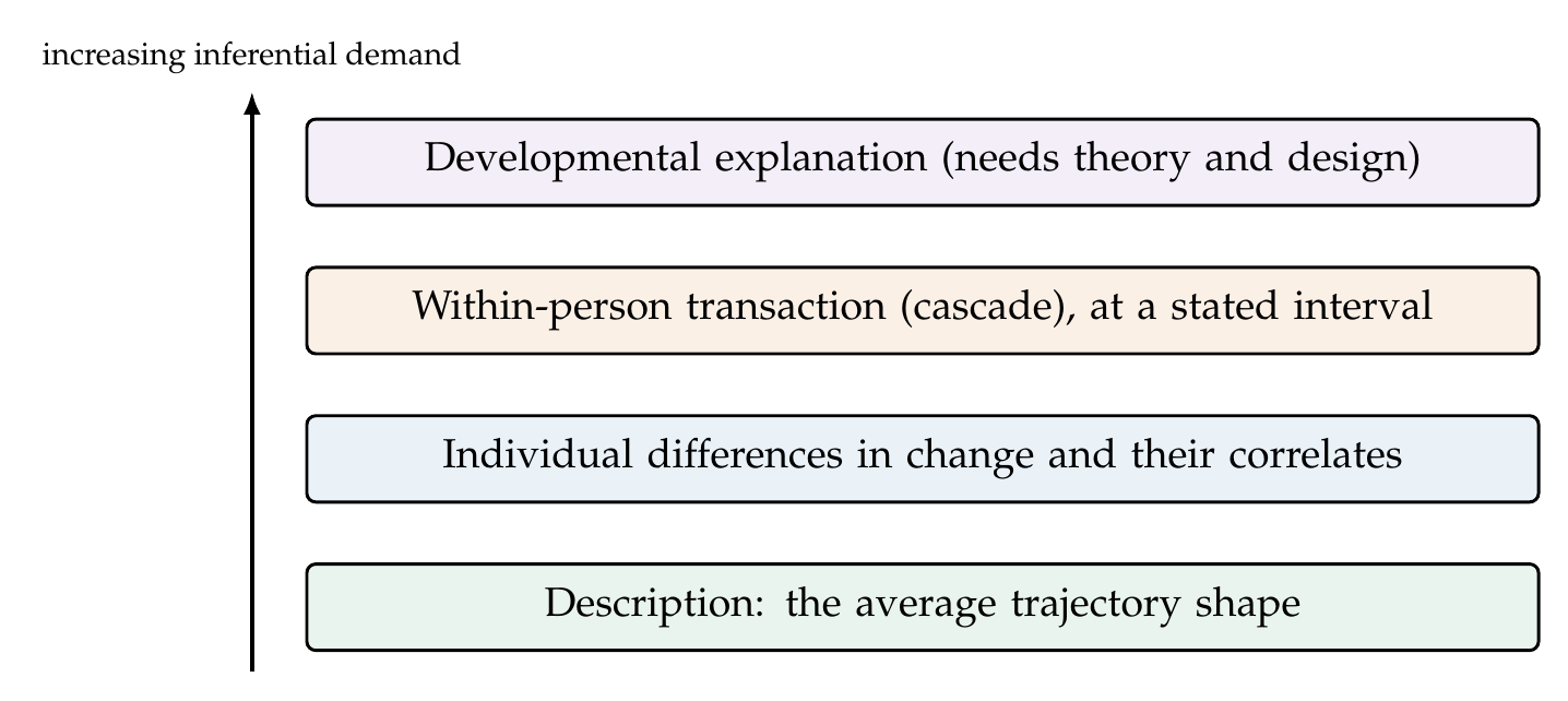
Note. Longitudinal data support claims unevenly. Description of average change is the most secure rung; individual differences and their correlates require sound measurement; within-person transactions require the trait-transaction separation and are interval-specific; developmental explanation requires theory and design beyond the panel itself. Locating a claim on the ladder is the discipline that keeps a longitudinal description from being oversold as a developmental explanation.
A reviewer for a developmental or educational journal will press on the domain’s characteristic vulnerabilities, and anticipating them is the analyst’s work. The reviewer will ask whether the time metric matches the estimand and whether the alternative was examined; whether the measure was shown invariant across the ages compared; whether the growth conclusion survives an alternative vertical scale; whether mobility was modeled rather than deleted; whether the accelerated design’s convergence was tested rather than assumed; whether a cascade claim rests on a model that separates trait from transaction; whether a variability-as-early-indicator claim is reported with its modest effect size and its attrition honestly handled; and whether a months-of-learning translation carries its scale and its caveat. Each of these is a place where the three case studies made a decision in the open, and the anchor literatures orient the reader who wants to go deeper: the achievement-growth and school-effects canon in Raudenbush and Bryk and in Bryk and Raudenbush, the vertical-scaling authority in Kolen and Brennan and its consequences in Briggs and Weeks, the cascade framing in Masten and Cicchetti and Sameroff with the estimand discipline in Curran and colleagues, and the aging-variability program in Ram and Gerstorf, MacDonald and colleagues, and the Lovden group. The domain that gave longitudinal methodology its first questions continues to pose its hardest measurement problems, and the craft it rewards is the one this chapter has tried to practice: to let the measurement decisions be seen, because in development they are not preliminaries to the science but part of it.
Software Note • Software Note
The analyses use only widely available packages. Growth and cross-classified models are fit with lme4, whose crossed random-effects syntax handles student mobility natively when the school identifier varies within child. Longitudinal invariance, the random-intercept cross-lagged panel model, and the bivariate latent change score model are fit with lavaan, the invariance sequence built by hand with the marker-variable method and freed factor means at the scalar step, because the automated invariance helpers in semTools were not required. The flexibility check uses mgcv. The vertical-scaling sensitivity, the burst-level inconsistency and autocorrelation, and the inverse-probability-of-attrition weighting are hand-rolled in base R, and the data generators and analysis scripts, seeded, accompany the chapter so that every figure in it can be reproduced against the planted truth.
Chapter Summary
Development and education are where longitudinal measurement is hardest, and this chapter’s lesson is that the measurement decisions precede and constrain the modeling. Case A carried an accelerated, school-nested achievement dataset through the measurement-to-policy chain, showing that the time metric follows the estimand, that invariance licenses the composite, that a vertical scale is a construction whose choice can reverse a growth conclusion or swing a gap-widening estimate sevenfold, that mobility must be modeled by cross-classification, that the accelerated design’s convergence is testable, and that a months-of-learning translation must carry its scale. Case B separated the stable trait from the within-person transaction, recovering a directional cascade with a random-intercept model that a conventional cross-lagged panel model compresses, and noted that a lagged effect is specific to its interval. Case C used a measurement-burst design to test whether variability precedes decline, finding the lead in the population and a modest person-level association, recovering a genuine increase in sluggish dynamics through the downward bias of short series, and correcting a survivor-biased mean by weighting for informative attrition. The developmental claims ladder locates each finding by its inferential demand, and the throughline is Wohlwill’s distinction between describing change and explaining development.
Baltes, P. B., & Nesselroade, J. R. (1979). History and rationale of longitudinal research. In J. R. Nesselroade & P. B. Baltes (Eds.), Longitudinal research in the study of behavior and development (pp. 1–39). Academic Press.
Briggs, D. C., & Weeks, J. P. (2009). The impact of vertical scaling decisions on growth interpretations. Educational Measurement: Issues and Practice, 28(4), 3–14. https://doi.org/10.1111/j.1745-3992.2009.00158.x
Bryk, A. S., & Raudenbush, S. W. (1988). Toward a more appropriate conceptualization of research on school effects: A three-level hierarchical linear model. American Journal of Education, 97(1), 65–108. https://doi.org/10.1086/443913
Curran, P. J., Howard, A. L., Bainter, S. A., Lane, S. T., & McGinley, J. S. (2014). The separation of between-person and within-person components of individual change over time: A latent curve model with structured residuals. Journal of Consulting and Clinical Psychology, 82(5), 879–894. https://doi.org/10.1037/a0035297
Duncan, T. E., & Duncan, S. C. (2009). The ABC’s of LGM: An introductory guide to latent variable growth curve modeling. Social and Personality Psychology Compass, 3(6), 979–991. https://doi.org/10.1111/j.1751-9004.2009.00224.x
Ferrer, E., Shaywitz, B. A., Holahan, J. M., Marchione, K., & Shaywitz, S. E. (2010). Uncoupling of reading and IQ over time: Empirical evidence for a definition of dyslexia. Psychological Science, 21(1), 93–101. https://doi.org/10.1177/0956797609354084
Grimm, K. J., An, Y., McArdle, J. J., Zonderman, A. B., & Resnick, S. M. (2012). Recent changes leading to subsequent changes: Extensions of multivariate latent difference score models. Structural Equation Modeling, 19(2), 268–292. https://doi.org/10.1080/10705511.2012.659627
Hertzog, C., Lindenberger, U., Ghisletta, P., & von Oertzen, T. (2006). On the power of multivariate latent growth curve models to detect correlated change. Psychological Methods, 11(3), 244–252. https://doi.org/10.1037/1082-989X.11.3.244
Hoffman, L., & Stawski, R. S. (2009). Persons as contexts: Evaluating between-person and within-person effects in longitudinal analysis. Research in Human Development, 6(2–3), 97–120. https://doi.org/10.1080/15427600902911189
Kolen, M. J., & Brennan, R. L. (2014). Test equating, scaling, and linking: Methods and practices (3rd ed.). Springer. https://doi.org/10.1007/978-1-4939-0317-7
Lövdén, M., Li, S.-C., Shing, Y. L., & Lindenberger, U. (2007). Within-person trial-to-trial variability precedes and predicts cognitive decline in old and very old age: Longitudinal data from the Berlin Aging Study. Neuropsychologia, 45(12), 2827–2838. https://doi.org/10.1016/j.neuropsychologia.2007.05.005
MacDonald, S. W. S., Hultsch, D. F., & Dixon, R. A. (2003). Performance variability is related to change in cognition: Evidence from the Victoria Longitudinal Study. Psychology and Aging, 18(3), 510–523. https://doi.org/10.1037/0882-7974.18.3.510
Masten, A. S., & Cicchetti, D. (2010). Developmental cascades. Development and Psychopathology, 22(3), 491–495. https://doi.org/10.1017/S0954579410000222
McArdle, J. J., & Epstein, D. (1987). Latent growth curves within developmental structural equation models. Child Development, 58(1), 110–133. https://doi.org/10.2307/1130295
Miyazaki, Y., & Raudenbush, S. W. (2000). Tests for linkage of multiple cohorts in an accelerated longitudinal design. Psychological Methods, 5(1), 44–63. https://doi.org/10.1037/1082-989X.5.1.44
Nesselroade, J. R. (1991). The warp and the woof of the developmental fabric. In R. M. Downs, L. S. Liben, & D. S. Palermo (Eds.), Visions of aesthetics, the environment & development: The legacy of Joachim F. Wohlwill (pp. 213–240). Lawrence Erlbaum Associates.
Ram, N., & Gerstorf, D. (2009). Time-structured and net intraindividual variability: Tools for examining the development of dynamic characteristics and processes. Psychology and Aging, 24(4), 778–791. https://doi.org/10.1037/a0017915
Raudenbush, S. W., & Bryk, A. S. (2002). Hierarchical linear models: Applications and data analysis methods (2nd ed.). Sage.
Salthouse, T. A. (2014). Why are there different age relations in cross-sectional and longitudinal comparisons of cognitive functioning? Current Directions in Psychological Science, 23(4), 252–256. https://doi.org/10.1177/0963721414535212
Sameroff, A. (Ed.). (2009). The transactional model of development: How children and contexts shape each other. American Psychological Association. https://doi.org/10.1037/11877-000
Schaie, K. W. (1965). A general model for the study of developmental problems. Psychological Bulletin, 64(2), 92–107. https://doi.org/10.1037/h0022371
Sliwinski, M. J. (2008). Measurement-burst designs for social health research. Social and Personality Psychology Compass, 2(1), 245–261. https://doi.org/10.1111/j.1751-9004.2007.00043.x
Tong, Y., & Kolen, M. J. (2007). Comparisons of methodologies and results in vertical scaling for educational achievement tests. Applied Measurement in Education, 20(2), 227–253. https://doi.org/10.1080/08957340701301207
Wohlwill, J. F. (1973). The study of behavioral development. Academic Press.