Dynamic missingness graphs: the motif taxonomy and recoverability

What a dm-graph is

A dynamic missingness graph (dm-graph) is a directed acyclic graph over the unrolled within-person process of an experience-sampling study. It extends the missingness graphs of Mohan and Pearl (2021) to repeated prompts: instead of one node per variable, the graph has one node per variable and prompt, and the missingness mechanism is a set of edges into the response indicators.

The nodes are

eta, the person’s typical state (a person-level latent variable; in estimation it is realized by person-specific intercepts);
X1, X2, ..., the momentary states at prompts 1, 2, …; the third prompt of the window is the focal prompt t, so X3 is X_t, X2 is X_t-1, and so on;
R1, R2, ..., the response indicators (1 = the prompt was answered, and the states are recorded);
optionally C (a context variable, latent or observed), S (an always-observed passive sensor), Z (a randomized probe that forces a response), zeta (a person-level response propensity) and U (a latent common cause of eta and zeta).

Two kinds of edges are always present: the dynamics X_{t-1} -> X_t and the person effect eta -> X_t. Everything else is a declaration about why prompts are skipped.

g <- dm_graph("M0")
g
#> Dynamic missingness graph (window of 5 prompts)
#>   motifs: M0 
#>   context: none  
#>   sensor: FALSE   probe: FALSE 
#>   nodes: 11   edges: 9
g$edges[1:6, ]
#>      from  to  
#> [1,] "eta" "X1"
#> [2,] "eta" "X2"
#> [3,] "eta" "X3"
#> [4,] "eta" "X4"
#> [5,] "eta" "X5"
#> [6,] "X1"  "X2"

The seven motifs

Each motif adds a specific set of edges. The codes are the ones used throughout the package (in dm_graph(), simulate_ema() and the printed reports).

Code	Name	Edges added	Substantive story
M0	completely random	none into `R`	a phone left in another room
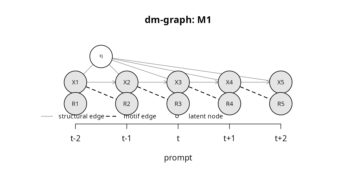
M1	lagged-state dependence	`X_{t-1} -> R_t`	high stress in the morning predicts skipping the afternoon prompt
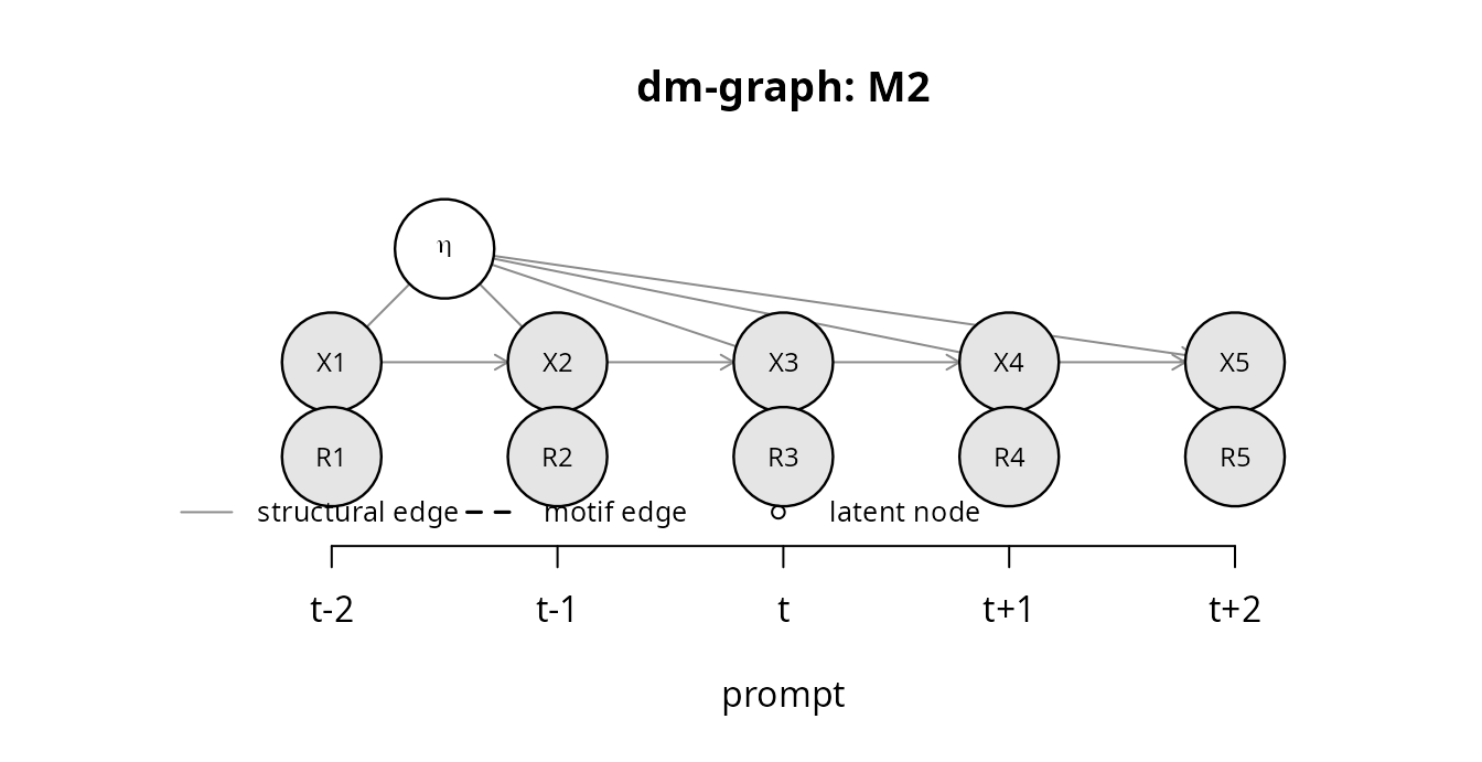
M2	self-censoring	`X_t -> R_t`	the current state itself causes the skip: too anxious to answer right now
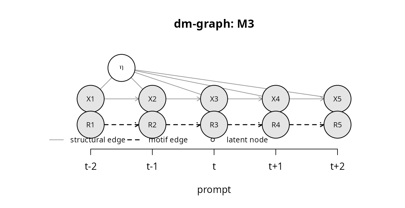
M3	burden or fatigue	`R_{t-1} -> R_t`	having skipped once makes skipping again more likely; compliance declines
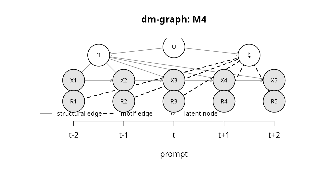
M4	person propensity	`zeta -> R_t`, `U -> eta`, `U -> zeta`	some people respond less, and they also differ in their typical states
M5	context confounding	`C_t -> X_t`, `C_t -> R_t`	being at work raises stress and lowers responding
M6	reactivity	`R_{t-1} -> X_t`	answering a prompt changes the next state (assessment reactivity)

The plots below draw each motif. Structural edges are gray and solid, motif edges are black and dashed, latent nodes are open circles.

for (m in c("M1", "M2", "M3")) plot(dm_graph(m))

for (m in c("M4", "M6")) plot(dm_graph(m))

plot(dm_graph("M5", context = "observed"))

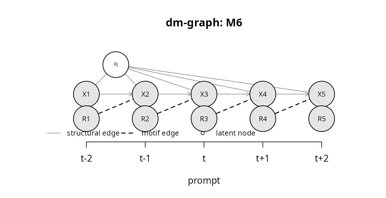
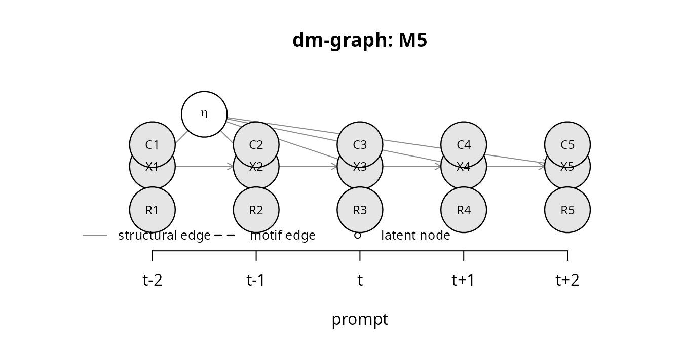
Motifs combine. dm_graph(c("M2", "M4")) declares self-censoring together with a person propensity; dm_graph(c("M1", "M3")) declares lagged-state dependence together with burden. A context is declared through context = "latent" or context = "observed" (which adds M5 automatically), and context_persistent = TRUE adds C_{t-1} -> C_t. Sensors and probes are design features rather than mechanisms and are declared through sensor = TRUE and probe = TRUE.

g <- dm_graph(c("M2", "M4"), sensor = TRUE, probe = TRUE)
g
#> Dynamic missingness graph (window of 5 prompts)
#>   motifs: M2 + M4 
#>   context: none  
#>   sensor: TRUE   probe: TRUE 
#>   nodes: 23   edges: 31
plot(g)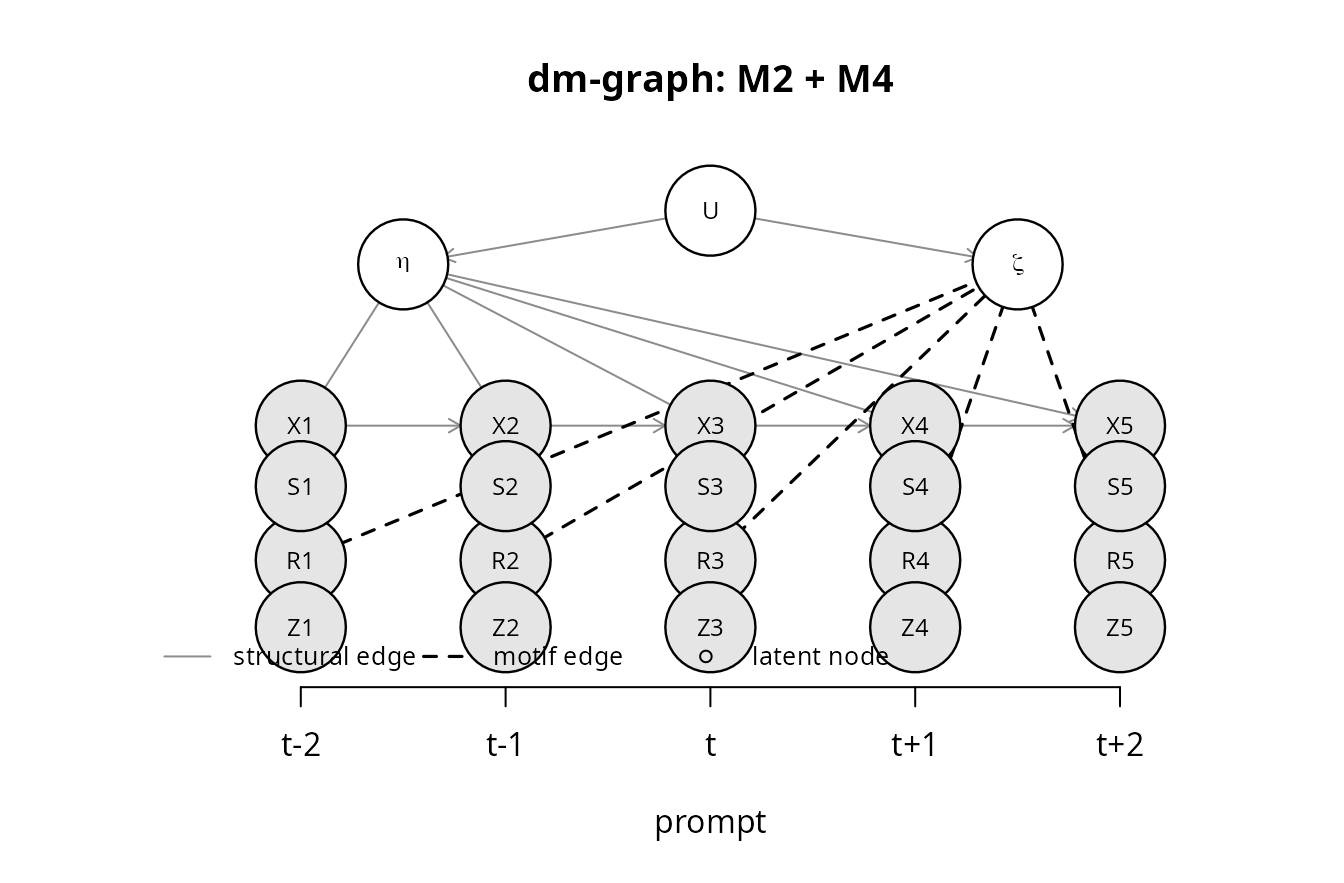

Asking the graph questions: d-separation

dsep() answers whether two sets of nodes are d-separated given a conditioning set, with the Bayes-ball algorithm (Shachter, 1998; Koller & Friedman, 2009). The central question for the transition kernel is whether the response indicator at t is independent of the state at t given the previous state and the person:

dsep(dm_graph("M1"), "R3", "X3", c("X2", "eta"))   # lagged-state dependence: yes
#> [1] TRUE
dsep(dm_graph("M2"), "R3", "X3", c("X2", "eta"))   # self-censoring: no
#> [1] FALSE
dsep(dm_graph("M4"), "R3", "X3", c("X2", "eta"))   # the person intercept blocks zeta -> R and U -> eta
#> [1] TRUE
dsep(dm_graph("M4"), "R3", "X3", "X2")             # without it, R and X are associated through U
#> [1] FALSE

dsep() works on any edge list, not only on dm-graphs, which makes it easy to check textbook cases:

chain <- list(nodes = c("A", "B", "C"), edges = cbind(from = c("A", "B"), to = c("B", "C")))
c(marginal = dsep(chain, "A", "C"), given_B = dsep(chain, "A", "C", "B"))
#> marginal  given_B 
#>    FALSE     TRUE
collider <- list(nodes = c("A", "B", "C"), edges = cbind(from = c("A", "C"), to = c("B", "B")))
c(marginal = dsep(collider, "A", "C"), given_B = dsep(collider, "A", "C", "B"))
#> marginal  given_B 
#>     TRUE    FALSE

The recoverability report

recoverability() applies the d-separation conditions derived in Yu (2026) to a declared graph and reports, for every estimand of the two-level VAR(1), whether it is structurally recoverable from the answered prompts and by which estimator. Recoverability is used in the sense of Mohan and Pearl (2021): there exists a consistent estimator that uses only the observed part of the data.

recoverability(dm_graph("M1"))
#> Recoverability report for motifs: M1 
#> 
#> * transition kernel (Phi, Psi, contemporaneous network)
#>     [recoverable] complete adjacent pairs, within-person (person intercepts)
#>     condition: R_t _||_ X_t | {X_{t-1},eta} and R_{t-1} _||_ X_t | {X_{t-1},eta, R_t}
#> * person mean via observed within-person mean
#>     [NOT recoverable] biased
#>     condition: R_t _||_ X_t | {eta}
#> * person mean via recovered dynamics
#>     [recoverable] mu_i = (I - Phi)^{-1} c_i from the recovered kernel
#>     condition: transition kernel recoverable
#> * between-person law (mu, Sigma_mu), person-weighted
#>     [recoverable] one recovered mean per person (dynamics-recovered means), persons weighted equally; positivity assumed
#>     condition: a person-mean estimator is available and P(R_t = 1 | eta) > 0
#> * between-person law, prompt-weighted (pooling answered prompts)
#>     [NOT recoverable] biased: response rate depends on the person's states
#>     condition: R_t _||_ X_t | {empty set}
#> * silence test (coefficient of R_t in X_{t+1} ~ X_{t-1} + R_t, within person)
#>     null expected (test valid as a test of the recoverable class)
#>     condition: R_t _||_ X_{t+1} | {X_{t-1},eta,R_{t-1},R_{t+1}}

The estimands are

the transition kernel (the lagged coefficients Phi, the innovation covariance Psi and hence the temporal and the contemporaneous network), recovered from complete adjacent pairs with person intercepts when R_t is independent of X_t given X_{t-1} and the person, and R_{t-1} is independent of X_t given the same set plus R_t;
the person mean read from the answered prompts, recovered when R_t is independent of X_t given the person;
the person mean recovered from the dynamics, mu_i = (I - Phi)^{-1} c_i, available whenever the kernel is recoverable and there is no reactivity;
the between-person law (mean vector and covariance of the person means), person-weighted, available whenever some person-mean estimator is;
the same law prompt-weighted (pooling answered prompts), which additionally needs R_t independent of X_t marginally; and
two rows that do not describe recoverability but the expected behavior of the silence test and (when a sensor is declared) the sensor-gap test under the graph: whether their null hypothesis is implied, so that a rejection speaks against the declared class.

A table over the taxonomy

The loop below reproduces the recoverability table of the accompanying article for all single motifs and the combinations that matter in practice.

decls <- list("M0", "M1", "M2", "M3", "M4", "M5", "M6", c("M1", "M3"), c("M1", "M4"),
              c("M3", "M4"), c("M2", "M4"), c("M2", "M3"))
tab <- do.call(rbind, lapply(decls, function(m) {
  r <- recoverability(dm_graph(m))
  data.frame(motifs = paste(m, collapse = "+"),
             kernel = r$recoverable[1], mean_obs = r$recoverable[2], mean_dyn = r$recoverable[3],
             law_person = r$recoverable[4], law_prompt = r$recoverable[5],
             silence_null = attr(r, "silence_null"))
}))
#> M5 declared without 'context': a latent context is assumed
tab
#>    motifs kernel mean_obs mean_dyn law_person law_prompt silence_null
#> 1      M0   TRUE     TRUE     TRUE       TRUE       TRUE         TRUE
#> 2      M1   TRUE    FALSE     TRUE       TRUE      FALSE         TRUE
#> 3      M2  FALSE    FALSE    FALSE      FALSE      FALSE        FALSE
#> 4      M3   TRUE     TRUE     TRUE       TRUE       TRUE         TRUE
#> 5      M4   TRUE     TRUE     TRUE       TRUE      FALSE         TRUE
#> 6      M5  FALSE    FALSE    FALSE      FALSE      FALSE        FALSE
#> 7      M6   TRUE     TRUE    FALSE       TRUE       TRUE        FALSE
#> 8   M1+M3   TRUE    FALSE     TRUE       TRUE      FALSE        FALSE
#> 9   M1+M4   TRUE    FALSE     TRUE       TRUE      FALSE         TRUE
#> 10  M3+M4   TRUE     TRUE     TRUE       TRUE      FALSE         TRUE
#> 11  M2+M4  FALSE    FALSE    FALSE      FALSE      FALSE        FALSE
#> 12  M2+M3  FALSE    FALSE    FALSE      FALSE      FALSE        FALSE

Three patterns organize the table.

M0, M1, M3, M4 and their combinations are recoverable. Skipping may depend on the previous state, on the previous response, or on a person’s stable propensity, and the answered adjacent pairs with person intercepts still recover the dynamics. Two casualties remain: under M1 (alone or combined) the observed within-person mean is biased, because skipping depends on the previous state, so the person mean must be recovered from the dynamics; and the prompt-weighted between-person law is biased under M1 and M4, whenever the response rate depends on a person’s states or on zeta.
M2 and latent M5 are not recoverable. Self-censoring and an unobserved context make R_t depend on X_t itself, and no conditioning set of observed variables blocks the path. Structural non-recoverability does not say how large the bias of a given estimator is: in the additive simulations of Yu (2026) the lagged coefficients are barely affected by a serially independent latent context (the shift lands in the intercepts) but are biased under a persistent one, while the means are biased in both cases, and under self-censoring everything is biased. This is where the sensitivity analysis of vignette("sensitivity-analysis") comes in.
M6 is asymmetric. Reactivity leaves the kernel recoverable (complete pairs estimate the assessment-conditioned kernel), but the intercept of the answered pairs absorbs the reactivity shift, so the person mean must be read from the answered prompts rather than from the dynamics.

The silence_null column shows where the silence test is a valid test of the recoverable class: everywhere among M0, M1, M3, M4 and their combinations except M1 + M3 (under M6 the kernel is recoverable, but reactivity makes the test reject by construction), where conditioning on an answered prompt at t + 1 opens a collider at R_{t+1}: its parents are R_t (burden) and X_t (lagged-state dependence), and X_t drives X_{t+1}. The report says so in words:

r13 <- recoverability(dm_graph(c("M1", "M3")))
r13$estimator[grepl("silence", r13$estimand)]
#> [1] "null violated although the kernel is recoverable (collider at R_{t+1}); use the sensor-gap test or check for fatigue first"

Observed contexts, sensors and probes

An observed context turns latent M5 into a recoverable mechanism: the context enters the conditioning set (covariate adjustment, fit_pairs(covariates = )), or the pairs are reweighted so that the context-marginal kernel is recovered (fit_ipw()).

recoverability(dm_graph("M5", context = "observed"))[1, c("recoverable", "estimator")]
#>   recoverable
#> 1        TRUE
#>                                                                                                           estimator
#> 1 complete pairs, context-conditional kernel (covariate adjustment); context-marginal kernel by stabilized IPW on C

A sensor adds the sensor-gap row, which is valid also under M1 + M3 because nothing is conditioned on at t + 1:

rs <- recoverability(dm_graph(c("M1", "M3"), sensor = TRUE))
rs$estimator[grepl("sensor", rs$estimand)]
#> [1] "null expected (test valid as a test of the recoverable class)"

A probe adds a row for the kernel estimated from probe prompts only. Because Z_t = 1 forces R_t = 1, complete pairs restricted to probe prompts are not selected on X_t even under self-censoring; this is what calibrate_delta(method = "probe") exploits.

rp <- recoverability(dm_graph("M2", probe = TRUE))
rp[rp$estimand == "transition kernel from probe prompts", c("recoverable", "estimator")]
#>   recoverable
#> 2        TRUE
#>                                                                                      estimator
#> 2 complete pairs restricted to probe prompts (Z_t = 1); delta calibrated by the probe contrast

Choosing a declaration in practice

The graph is a declaration, not a finding: it records what the analyst is willing to assume about why prompts were skipped, and recoverability() says what follows. A workable procedure is

start from the design: are there always-observed channels (sensor), forced-response prompts (probe), recorded contexts?
declare the mechanisms that the design and the pilot evidence make plausible (compliance patterns by time of day suggest M1 or M5; declining compliance suggests M3; people with low compliance differing in level suggests M4; content that is aversive to report suggests M2);
read the report; if the kernel is recoverable, estimate with fit_pairs() and run the tests of vignette("testing-informativeness") as checks; if not, run the sensitivity analysis;
record the declaration with missingness_declaration().

References

Koller, D., & Friedman, N. (2009). Probabilistic graphical models: Principles and techniques. MIT Press.

Mohan, K., & Pearl, J. (2021). Graphical models for processing missing data. Journal of the American Statistical Association, 116, 1023-1037. https://doi.org/10.1080/01621459.2021.1874961

Shachter, R. D. (1998). Bayes-ball: The rational pastime. In Proceedings of the Fourteenth Conference on Uncertainty in Artificial Intelligence (pp. 480-487). Morgan Kaufmann.

Yu, H.-T. (2026). What skipped prompts hide: Detecting, diagnosing, and correcting informative nonresponse in ecological momentary assessment. Manuscript under review.

Hsiu-Ting Yu