Getting started: the silentema workflow
Hsiu-Ting Yu
Source:vignettes/silentema-workflow.Rmd
silentema-workflow.RmdExperience-sampling participants skip prompts, and the reasons are
rarely unrelated to the states being measured. silentema
provides a graphical language for saying which mechanism is assumed (a
dynamic missingness graph), a checker that says which quantities of a
two-level VAR(1) remain estimable under that mechanism, two tests that
ask the data whether skipped prompts were informative, and a sensitivity
analysis for the one mechanism that cannot be repaired by estimation
alone: self-censoring, where the current state itself causes the skip.
This vignette walks through one complete analysis on simulated data. The
other vignettes go deeper into each step:
vignette("dm-graphs"),
vignette("testing-informativeness"),
vignette("sensitivity-analysis") and
vignette("simulation-and-design").
0. The data format
Every estimator takes a long data frame with one row per scheduled prompt, answered or not:
| Column | Content |
|---|---|
id |
person identifier |
time |
integer prompt index, increasing by one from one scheduled prompt to the next within a person |
R |
response indicator, 1 = answered (if absent, a prompt counts as answered when all state columns are non-missing) |
| state columns | the momentary states, NA at skipped prompts |
day (optional) |
day index; adjacent pairs are then formed within days only, so the overnight gap is not treated as a lag-1 transition |
| sensor, probe, context (optional) | an always-observed channel, a forced-response indicator, recorded contexts |
Rows for skipped prompts must be present (with R = 0 and
NA states): the tests and the response models need to know
that a prompt was scheduled and skipped. Two rows whose
time values differ by more than one are not adjacent. Real
data usually need a reshaping step to reach this format;
simulate_ema() produces it directly.
1. Simulate a study with self-censoring
library(silentema)
sim <- simulate_ema(N = 60, n_prompts = 40, motifs = "M2", compliance = 0.70, delta = -1,
                    sensor_cor = 0.6, p_probe = 0.05, days = 5, seed = 1)
sim
#> Simulated EMA data: 60 persons x 40 prompts, 4 variables
#>   motifs: M2   realized response rate: 0.7
head(sim$data)
#>   id time day R         NegA     PosA      Stress  Fatigue          S Z
#> 1  1    1   1 1  1.936136574 4.844164  0.92785937 1.299934 -0.7399196 0
#> 2  1    2   1 1  1.584265346 4.232716 -0.06654146 3.908155  1.0259370 0
#> 3  1    3   1 1  0.006044839 4.811683  0.09100665 2.370911 -0.3047950 1
#> 4  1    4   1 1 -0.135652698 3.759730  2.40007772 4.401480 -1.3248360 0
#> 5  1    5   1 1 -1.452317972 3.684295  0.51494056 3.981258 -0.9807267 0
#> 6  1    6   2 1 -0.496998276 6.128918  0.43275347 4.684704 -2.1736344 0
Four momentary states (negative affect, positive affect, stress,
fatigue) follow a two-level VAR(1) with person-specific means. Prompts
are answered with a probit probability that decreases in the current
level of negative affect (delta = -1), so the
high-negative-affect moments are the ones that get skipped. A passive
sensor correlated .6 with the within-person fluctuations of negative
affect is observed at every prompt, and 5% of prompts are randomized
probes that are always answered. Eight days of five prompts each.
2. Declare a dynamic missingness graph and check recoverability
g <- dm_graph(motifs = "M2", sensor = TRUE, probe = TRUE)
g
#> Dynamic missingness graph (window of 5 prompts)
#>   motifs: M2
#>   context: none
#>   sensor: TRUE   probe: TRUE
#>   nodes: 21   edges: 24
plot(g)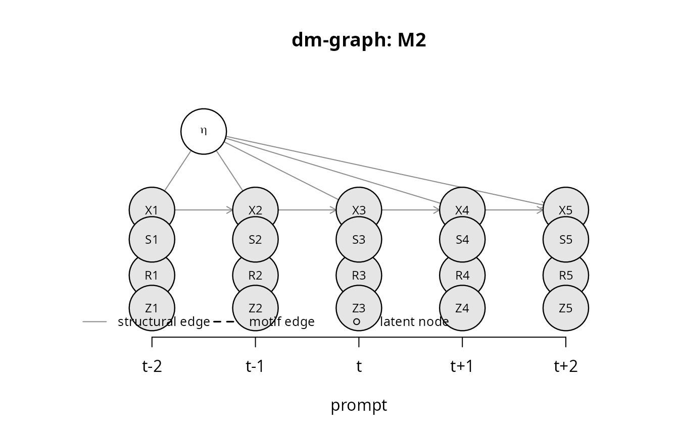
recoverability(g)
#> Recoverability report for motifs: M2
#>
#> * transition kernel (Phi, Psi, contemporaneous network)
#>     [NOT recoverable] sensitivity analysis (tilt profile) or a calibration design is required
#>     condition: R_t and X_t are d-connected given {X_{t-1},eta}
#> * transition kernel from probe prompts
#>     [recoverable] complete pairs restricted to probe prompts (Z_t = 1); delta calibrated by the probe contrast
#>     condition: Z_t _||_ X_t | {X_{t-1},eta}; R_t = 1 whenever Z_t = 1
#> * person mean via observed within-person mean
#>     [NOT recoverable] biased
#>     condition: R_t _||_ X_t | {eta}
#> * person mean via recovered dynamics
#>     [NOT recoverable] not available
#>     condition: transition kernel recoverable
#> * between-person law (mu, Sigma_mu), person-weighted
#>     [NOT recoverable] not recoverable
#>     condition: a person-mean estimator is available and P(R_t = 1 | eta) > 0
#> * between-person law, prompt-weighted (pooling answered prompts)
#>     [NOT recoverable] biased: response rate depends on the person's states
#>     condition: R_t _||_ X_t | {empty set}
#> * silence test (coefficient of R_t in X_{t+1} ~ X_{t-1} + R_t, within person)
#>     non-null expected: silence is informative
#>     condition: R_t _||_ X_{t+1} | {X_{t-1},eta,R_{t-1},R_{t+1}}
#> * sensor-gap test (coefficient of R_t in S_t ~ X_{t-1} + R_t, within person)
#>     non-null expected: delta can be calibrated from the sensor gap
#>     condition: R_t _||_ S_t | {X_{t-1},eta,R_{t-1}}
The report says that the transition kernel (and therefore the temporal and contemporaneous networks) is not structurally recoverable under self-censoring, that the silence test and the sensor-gap test are expected to reject, and that the kernel can be recovered from probe prompts. Compare with a recoverable mechanism and with reactivity, under which the dynamics are recovered but the person mean must be read from the answered prompts rather than from the dynamics:
recoverability(dm_graph(c("M1", "M4")))
#> Recoverability report for motifs: M1 + M4
#>
#> * transition kernel (Phi, Psi, contemporaneous network)
#>     [recoverable] complete adjacent pairs, within-person (person intercepts)
#>     condition: R_t _||_ X_t | {X_{t-1},eta,zeta} and R_{t-1} _||_ X_t | {X_{t-1},eta,zeta, R_t}
#> * person mean via observed within-person mean
#>     [NOT recoverable] biased
#>     condition: R_t _||_ X_t | {eta,zeta}
#> * person mean via recovered dynamics
#>     [recoverable] mu_i = (I - Phi)^{-1} c_i from the recovered kernel
#>     condition: transition kernel recoverable
#> * between-person law (mu, Sigma_mu), person-weighted
#>     [recoverable] one recovered mean per person (dynamics-recovered means), persons weighted equally; positivity assumed
#>     condition: a person-mean estimator is available and P(R_t = 1 | eta) > 0
#> * between-person law, prompt-weighted (pooling answered prompts)
#>     [NOT recoverable] biased: response rate depends on the person's states
#>     condition: R_t _||_ X_t | {empty set}
#> * silence test (coefficient of R_t in X_{t+1} ~ X_{t-1} + R_t, within person)
#>     null expected (test valid as a test of the recoverable class)
#>     condition: R_t _||_ X_{t+1} | {X_{t-1},eta,zeta,R_{t-1},R_{t+1}}
recoverability(dm_graph("M6"))
#> Recoverability report for motifs: M6
#>
#> * transition kernel (Phi, Psi, contemporaneous network)
#>     [recoverable] complete adjacent pairs recover the assessment-conditioned kernel p(X_t | X_{t-1}, eta, R_{t-1} = 1): Phi and Psi are unaffected when reactivity shifts the level (additive), but the person intercept absorbs the shift
#>     condition: reactivity edge R_{t-1} -> X_t declared; all complete pairs have R_{t-1} = 1
#> * person mean via observed within-person mean
#>     [recoverable] mean of answered prompts, per person
#>     condition: R_t _||_ X_t | {eta}
#> * person mean via recovered dynamics
#>     [NOT recoverable] biased: the answered-pair intercept is the intercept of the assessed process (it absorbs the reactivity shift)
#>     condition: transition kernel recoverable and no reactivity
#> * between-person law (mu, Sigma_mu), person-weighted
#>     [recoverable] one recovered mean per person (observed means), persons weighted equally; positivity assumed
#>     condition: a person-mean estimator is available and P(R_t = 1 | eta) > 0
#> * between-person law, prompt-weighted (pooling answered prompts)
#>     [recoverable] pooled answered prompts
#>     condition: R_t _||_ X_t | {empty set}
#> * silence test (coefficient of R_t in X_{t+1} ~ X_{t-1} + R_t, within person)
#>     non-null expected: silence is informative
#>     condition: R_t _||_ X_{t+1} | {X_{t-1},eta,R_{t-1},R_{t+1}}
3. Ask the data whether silence was informative
st <- silence_test(sim$data, sim$vars, day = "day")
st
#> Silence test: X_{t+1} ~ X_{t-1} + R_t (within person), 757 triples, 142 with a skipped middle prompt
#>  variable coef_R    se     z       p
#>      NegA -0.279 0.095 -2.94 0.00470
#>      PosA  0.230 0.093  2.48 0.01600
#>    Stress -0.353 0.094 -3.76 0.00039
#>   Fatigue  0.051 0.120  0.43 0.67000
#> Joint Wald test: statistic = 18.86 on 4 df, p = 0.00227   [SE: cluster; t / F with G - 1 df reference]
#> Interpretation: coefficients near zero are expected under the recoverable motifs; a negative coefficient on a variable means the states hidden by skips were higher.
sg <- sensor_gap_test(sim$data, sim$vars, sensor = "S", day = "day")
sg
#> Sensor-gap test: S_t ~ X_{t-1} + R_t (within person), 1336 prompts with answered predecessor
#>   coefficient of R_t: -0.440 (SE 0.062), z = -7.12, p = 1.67e-09   [SE: cluster]
#>   sensor loading on states (answered prompts): 0.637 -0.007 0.002 0.001
fatigue_check(sim$data, day = "day")
#> Fatigue check over 1920 consecutive prompts
#>   response rate after an answered prompt: 0.770; after a skipped prompt: 0.563; difference 0.207 (person-mean difference 0.090)
#>   response rate by study quarter: 0.695 0.693 0.707 0.705
The coefficient of R_t on negative affect in the silence
test and the sensor gap are both negative: the states hidden by skipped
prompts were higher than the reported ones. The positive coefficient on
positive affect is the same tilt seen through the negative
contemporaneous association between the two. The fatigue check reports
the response persistence that burden (M3) would produce: here the pooled
contrast is inflated by between-person differences in response rate
(self-censoring acts on the raw state, so persons with a high typical
level respond less), while the person-mean contrast is modest and arises
from the autocorrelated states, as expected without burden.
4. Estimate, profile, calibrate
fit0 <- fit_pairs(sim$data, sim$vars, day = "day")
fit0
#> Within-person VAR(1) from 1029 complete adjacent pairs, 60 persons (half-panel jackknife)
#> Lagged coefficients Phi (rows = outcome at t, columns = predictor at t-1):
#>           NegA   PosA Stress Fatigue
#> NegA     0.357 -0.001  0.050   0.041
#> PosA    -0.023  0.304 -0.007  -0.055
#> Stress   0.139 -0.060  0.370   0.129
#> Fatigue  0.018 -0.113 -0.034   0.335
#> Contemporaneous partial correlations (innovations):
#>           NegA   PosA Stress Fatigue
#> NegA     1.000 -0.289  0.228   0.052
#> PosA    -0.289  1.000 -0.001  -0.055
#> Stress   0.228 -0.001  1.000   0.173
#> Fatigue  0.052 -0.055  0.173   1.000
#> Between-person means (dynamics-recovered): 1.934 4.218 2.573 2.949
confint(fit0)[1:4, ]
#>                      2.5 %     97.5 %
#> NegA<-NegA     0.280871621 0.43223611
#> NegA<-PosA    -0.053062748 0.05109106
#> NegA<-Stress  -0.007243953 0.10639392
#> NegA<-Fatigue -0.020598477 0.10212502
prof <- tilt_profile(sim$data, sim$vars, delta_grid = seq(-2, 0.5, by = 0.5), day = "day", probe = "Z")
prof
#> Tilt profile over delta in { -2, -1.5, -1, -0.5, 0, 0.5 } for NegA
#> Autoregressive coefficient of the self-censoring variable along the grid ( 1029 complete pairs):
#>  delta estimate lower upper  ess converged
#>   -2.0    0.489 0.378 0.601  552      TRUE
#>   -1.5    0.450 0.350 0.550  783      TRUE
#>   -1.0    0.403 0.316 0.490  925      TRUE
#>   -0.5    0.366 0.289 0.443 1008      TRUE
#>    0.0    0.357 0.281 0.432 1029      TRUE
#>    0.5    0.394 0.293 0.495  990      TRUE
plot(prof, plausible = c(-1.5, -0.5))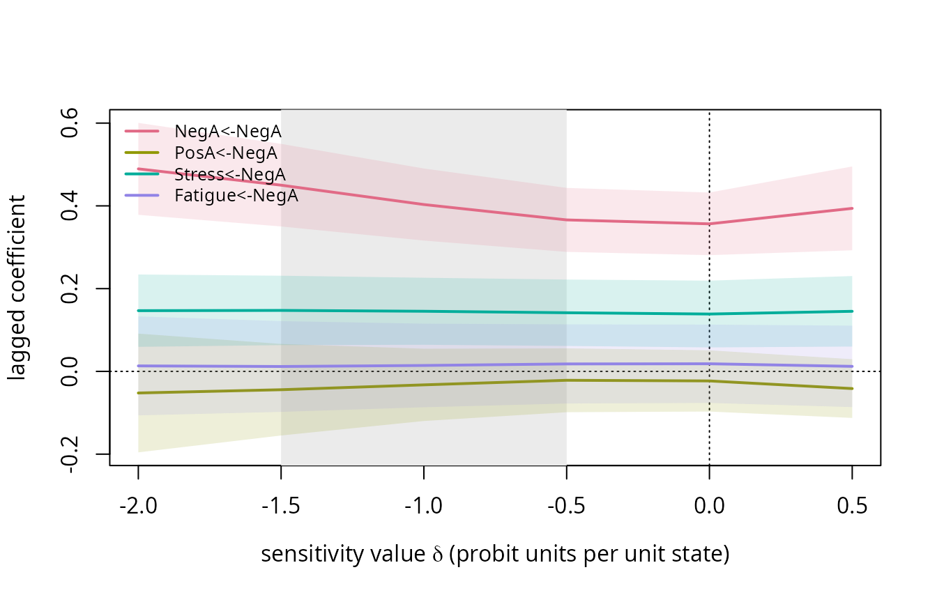
The autoregressive coefficient of negative affect rises as the analysis allows for stronger self-censoring; at the generating value (-1) it is close to the population value of .40. Three designs calibrate the sensitivity value:
cs <- calibrate_delta(prof, sim$data, method = "sensor", day = "day")
cs
#> Calibration of delta (NegA) by the sensor method
#>   observed statistic: -0.440 (SE 0.062)
#>   calibrated delta: -0.740   95% interval: [-0.967, -0.512]
plot(cs)
calibrate_delta(prof, sim$data, method = "probe", day = "day")
#> Calibration of delta (NegA) by the probe method
#>   observed statistic: 0.241 (SE 0.099)
#>   calibrated delta: -1.192   95% interval: [-Inf, -0.198]
The sensor calibration is the most precise of the three designs, but it is not immune to sampling variability: in this sample its interval stops short of the generating value of -1, whereas the probe calibration (with only 5% probes) is much less precise and its interval is open on one side. Yu (2026) reports the coverage of these intervals over many replications; a single study should report all available calibrations and let the plausible interval cover their union.
The post-skip contrast needs no extra channel but relies fully on the
functional form (it simulates from each fitted model; n_sim
controls the number of simulated data sets per grid value, and
burden = "fit" adds a burden term calibrated to the
observed response persistence when M3 is declared together with M2):
calibrate_delta(prof, sim$data, method = "postskip", day = "day", n_sim = 5, seed = 2)
#> Calibration of delta (NegA) by the postskip method
#>   observed statistic: -0.279 (SE 0.095)
#>   calibrated delta: -0.964   95% interval: [-Inf, -0.176]
5. Report
break_even(prof, delta_max = 1.5)[1:4, ]
#>               coef  estimate_0 significant_0 sign_flip_delta
#> 1 Fatigue<-Fatigue  0.33537104          TRUE              NA
#> 2    Fatigue<-NegA  0.01843167         FALSE              NA
#> 3    Fatigue<-PosA -0.11254432          TRUE              NA
#> 4  Fatigue<-Stress -0.03362374         FALSE              NA
#>   significance_flip_delta   set_lower   set_upper  band_lower  band_upper
#> 1                      NA  0.32322915  0.33948482  0.25950306  0.40066046
#> 2                      NA  0.01184862  0.01843167 -0.09782638  0.12152362
#> 3                      NA -0.12334249 -0.10889865 -0.21130170 -0.02099467
#> 4                      NA -0.03700220 -0.02996109 -0.11256409  0.05171477
cat(missingness_declaration(g, silence = st, sensor_gap = sg, profile = prof, calibration = cs,
                            plausible = c(-1.5, -0.5)), sep = "\n")
#> # Missingness declaration (silentema)
#>
#> ## 1. Design facts
#> - Prompts per day, days, scheduling, and the definition of a scheduled prompt: [to complete]
#> - Response rate overall and by person (median, range): [to complete]
#> - Whether prompt-level (whole prompt) or item-level missingness occurs: [to complete]
#>
#> ## 2. Declared dynamic missingness graph
#> - Motifs: M2
#> - Context: none
#> - Passive sensor available: TRUE; randomized probes: TRUE
#> - Substantive justification for each declared edge (cite compliance evidence or pilot data): [to complete]
#>
#> ## 3. Recoverability verdicts
#> - transition kernel (Phi, Psi, contemporaneous network): NOT recoverable; sensitivity analysis (tilt profile) or a calibration design is required
#> - transition kernel from probe prompts: recoverable; complete pairs restricted to probe prompts (Z_t = 1); delta calibrated by the probe contrast
#> - person mean via observed within-person mean: NOT recoverable; biased
#> - person mean via recovered dynamics: NOT recoverable; not available
#> - between-person law (mu, Sigma_mu), person-weighted: NOT recoverable; not recoverable
#> - between-person law, prompt-weighted (pooling answered prompts): NOT recoverable; biased: response rate depends on the person's states
#> - silence test (coefficient of R_t in X_{t+1} ~ X_{t-1} + R_t, within person): non-null expected: silence is informative
#> - sensor-gap test (coefficient of R_t in S_t ~ X_{t-1} + R_t, within person): non-null expected: delta can be calibrated from the sensor gap
#>
#> ## 4. Tests of informativeness
#> - Silence test (757 triples, 142 with a skipped middle prompt; SE: cluster):
#>     - NegA: coefficient of R_t = -0.279 (SE 0.095), p = 0.0047
#>     - PosA: coefficient of R_t = 0.230 (SE 0.093), p = 0.016
#>     - Stress: coefficient of R_t = -0.353 (SE 0.094), p = 0.00039
#>     - Fatigue: coefficient of R_t = 0.051 (SE 0.120), p = 0.67
#>     - joint test: statistic 18.863 on 4 df, p = 0.0023
#> - Sensor-gap test: coefficient of R_t = -0.440 (SE 0.062), p = 1.7e-09
#> - Fatigue check (response rate after answered vs skipped prompt; by study quarter): [to complete]
#>
#> ## 5. Sensitivity analysis
#> - Sensitivity parameter: delta, probit units per unit of NegA; grid {-2, -1.5, -1, -0.5, 0, 0.5}; response-model intercept: common
#> - Effective number of complete pairs along the grid: 552, 783, 925, 1008, 1029, 990 (of 1029)
#> - Calibration by the sensor method: delta = -0.740, 95% interval [-0.967, -0.512]
#> - Plausible interval used for the band: [-1.500, -0.500]
#> - Identified set and band over the plausible interval (effects of the self-censoring variable):
#>     - Fatigue<-NegA: estimate at delta = 0: 0.018; set [0.012, 0.018]; band [-0.098, 0.122]; sign change at none on the grid; significance change at none on the grid
#>     - NegA<-NegA: estimate at delta = 0: 0.357; set [0.357, 0.450]; band [0.281, 0.550]; sign change at none on the grid; significance change at none on the grid
#>     - PosA<-NegA: estimate at delta = 0: -0.023; set [-0.044, -0.021]; band [-0.155, 0.066]; sign change at none on the grid; significance change at none on the grid
#>     - Stress<-NegA: estimate at delta = 0: 0.139; set [0.139, 0.147]; band [0.058, 0.231]; sign change at none on the grid; significance change at none on the grid
#>
#> ## 6. What is reported in the paper
#> - Estimates under the declared graph, the sensitivity band, and this declaration.
break_even() returns, for every lagged coefficient, the
sensitivity value at which its sign or its significance would change,
and the range of estimates over the plausible interval (the identified
set). missingness_declaration() writes the declaration that
the accompanying article recommends for preregistrations and reports,
filling the sections for which objects are supplied.
6. Full-information maximum likelihood under missing at random
For comparison, the likelihood that dynamic structural equation models maximize:
fit_fiml(sim$data, sim$vars)
#> FIML (MAR) two-level VAR(1) by state-space EM: 60 persons, 40 prompts; 7 iterations, converged
#> Lagged coefficients Phi:
#>           NegA   PosA Stress Fatigue
#> NegA     0.358  0.006  0.100   0.037
#> PosA    -0.065  0.325 -0.009  -0.042
#> Stress   0.163 -0.031  0.410   0.153
#> Fatigue -0.005 -0.091  0.021   0.324
#> Contemporaneous partial correlations:
#>           NegA   PosA Stress Fatigue
#> NegA     1.000 -0.306  0.250   0.044
#> PosA    -0.306  1.000 -0.005  -0.018
#> Stress   0.250 -0.005  1.000   0.161
#> Fatigue  0.044 -0.018  0.161   1.000
#> Means: 2.082 4.149 2.752 2.95
Under self-censoring this estimator is biased in the same direction as the answered-pairs estimator, because both treat the mechanism as ignorable.
Where to go next
- Which mechanism to declare, and what follows from it:
vignette("dm-graphs"). - How the tests work, their power and their failure modes:
vignette("testing-informativeness"). - Tilting, break-even values, calibration and reporting in depth:
vignette("sensitivity-analysis"). - Planning a study with the simulator:
vignette("simulation-and-design"). - The accompanying article (Yu, 2026) and its archived materials: https://osf.io/x6d2t/.