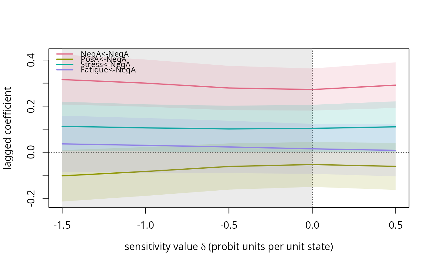
Fits fit_tilt over a grid of sensitivity values and collects
the lagged coefficients with cluster-robust confidence limits, the
contemporaneous partial correlations and the between-person means.
Arguments
- data
Long data frame with one row per scheduled prompt.
- vars
Names of the state columns.
- delta_grid
Numeric vector of values of the sensitivity parameter for the self-censoring variable (the first of
varsunlesswhichsays otherwise).- which
Index (in
vars), or name, of the variable that drives self-censoring.- id, time
Names of the person and prompt-index columns.
- day
Optional name of a day column; pairs are formed only within a day (the overnight gap is not a lag-1 transition).
- R
Name of the response-indicator column (0/1, no
NA). If the default name is not among the columns ofdata, a prompt counts as answered when allvarsare non-missing; any other name must exist.- propensity
"common"(one intercept) or"person"(one intercept per person; use when a person-propensity motif M4 is declared together with M2).- level
Confidence level for the limits.
- pairs
Optional precomputed result of
make_pairs.- probe
Optional probe column name passed to
fit_tilt.- min_pairs
Passed to
fit_pairs.
Value
An object of class "tilt_profile": a list with
delta_grid, which, vars, a data frame Phi
(one row per grid value and lagged coefficient, with coef,
estimate, se, lower, upper, z,
p and delta), a data frame pcor (contemporaneous
partial correlations by grid value and edge), a matrix mu
(between-person means by grid value), fits (the list of
fit_tilt objects), level, propensity,
converged and ess (one entry per grid value) and
n_pairs. Methods: print and
plot.
Examples
sim <- simulate_ema(N = 40, n_prompts = 30, motifs = "M2", delta = -1, seed = 1)
prof <- tilt_profile(sim$data, sim$vars, delta_grid = c(-1.5, -1, -0.5, 0, 0.5))
prof
#> Tilt profile over delta in { -1.5, -1, -0.5, 0, 0.5 } for NegA
#> Autoregressive coefficient of the self-censoring variable along the grid ( 709 complete pairs):
#>  delta estimate lower upper ess converged
#>   -1.5    0.315 0.207 0.424 587      TRUE
#>   -1.0    0.300 0.197 0.402 662      TRUE
#>   -0.5    0.279 0.183 0.375 699      TRUE
#>    0.0    0.272 0.181 0.363 709      TRUE
#>    0.5    0.291 0.192 0.390 688      TRUE
head(prof$Phi)
#>                coef    estimate         se      lower       upper          z
#> 16 Fatigue<-Fatigue  0.30269674 0.05137436  0.1987823  0.40661120  5.8919804
#> 13    Fatigue<-NegA  0.03620804 0.06042640 -0.0860159  0.15843197  0.5992089
#> 14    Fatigue<-PosA -0.14421602 0.04099723 -0.2271407 -0.06129130 -3.5177018
#> 15  Fatigue<-Stress -0.02361651 0.04231078 -0.1091981  0.06196512 -0.5581678
#> 4     NegA<-Fatigue -0.06730765 0.05125879 -0.1709883  0.03637304 -1.3130947
#> 1        NegA<-NegA  0.31539752 0.05357164  0.2070386  0.42375639  5.8873966
#>               p delta
#> 16 7.316475e-07  -1.5
#> 13 5.524988e-01  -1.5
#> 14 1.122534e-03  -1.5
#> 15 5.799203e-01  -1.5
#> 4  1.968249e-01  -1.5
#> 1  7.424540e-07  -1.5
prof$mu
#>          NegA     PosA   Stress  Fatigue
#> [1,] 2.475511 3.738218 2.902944 3.007834
#> [2,] 2.369494 3.833369 2.848691 2.991113
#> [3,] 2.247611 3.935126 2.786332 2.976697
#> [4,] 2.089641 4.036332 2.697751 2.953323
#> [5,] 1.876792 4.140249 2.570519 2.912625
break_even(prof, delta_max = 1)
#>                coef  estimate_0 significant_0 sign_flip_delta
#> 1  Fatigue<-Fatigue  0.32003947          TRUE              NA
#> 2     Fatigue<-NegA  0.01475191         FALSE              NA
#> 3     Fatigue<-PosA -0.10382720          TRUE              NA
#> 4   Fatigue<-Stress -0.00630844         FALSE             0.5
#> 5     NegA<-Fatigue -0.04273611         FALSE              NA
#> 6        NegA<-NegA  0.27202999          TRUE              NA
#> 7        NegA<-PosA -0.04336865         FALSE              NA
#> 8      NegA<-Stress  0.21222503          TRUE              NA
#> 9     PosA<-Fatigue  0.11721566          TRUE              NA
#> 10       PosA<-NegA -0.05327674         FALSE              NA
#> 11       PosA<-PosA  0.43526919          TRUE              NA
#> 12     PosA<-Stress -0.02393339         FALSE              NA
#> 13  Stress<-Fatigue  0.13098561          TRUE              NA
#> 14     Stress<-NegA  0.10342712          TRUE              NA
#> 15     Stress<-PosA -0.04538176         FALSE              NA
#> 16   Stress<-Stress  0.46173006          TRUE              NA
#>    significance_flip_delta    set_lower   set_upper    band_lower  band_upper
#> 1                       NA  0.307040198  0.32003947  0.2059476162  0.41859753
#> 2                       NA  0.007946694  0.02978227 -0.1046858801  0.14842800
#> 3                       NA -0.133116375 -0.09887209 -0.2145342477 -0.01311113
#> 4                       NA -0.017306828  0.01357034 -0.1018740059  0.11208303
#> 5                       NA -0.057794829 -0.04273611 -0.1480241841  0.04033494
#> 6                       NA  0.272029988  0.29988399  0.1807127461  0.40228824
#> 7                       NA -0.061535982 -0.02248452 -0.1454695785  0.05635852
#> 8                       NA  0.212225030  0.27055030  0.1416975325  0.36314900
#> 9                     -1.5  0.113184396  0.12575984  0.0068780914  0.21949070
#> 10                      NA -0.083562454 -0.05327674 -0.1894808339  0.04406566
#> 11                      NA  0.433224038  0.43638768  0.3386263979  0.52782168
#> 12                      NA -0.050280232 -0.02393339 -0.1845678217  0.09543843
#> 13                      NA  0.130738024  0.13318246  0.0642775092  0.20192544
#> 14                     0.5  0.101125068  0.11028455 -0.0002670581  0.22083617
#> 15                      NA -0.048516500 -0.04457373 -0.1026036788  0.00811859
#> 16                      NA  0.461730062  0.47363099  0.3694950042  0.55989895
plot(prof, plausible = c(-1.5, 0))