Likelihood, REML, and Empirical Bayes Derivations

Chapters 9, 11, 12, and 23 state results whose derivations would interrupt them. This appendix gives those derivations for the linear mixed model ${\mathbf{y}}_j={\mathbf{X}}_j\mathbf{\gamma }+{\mathbf{Z}}_j{\mathbf{u}}_j+{\mathbf{e}}_j$ with ${\mathbf{u}}_j\sim \mathcal{N}(0,\mathbf{T})$, ${\mathbf{e}}_j\sim \mathcal{N}(0,{\sigma }^2\mathbf{I})$, and marginal covariance ${\mathbf{V}}_j={\mathbf{Z}}_j\mathbf{T}{\mathbf{Z}}_j^{\prime }+{\sigma }^2\mathbf{I}$, in the notation of Appendix A, and extends them to generalized linear mixed models. Symbols without the subscript $j$ refer to all clusters together: $\mathbf{y}$ and $\mathbf{X}$ stack the ${\mathbf{y}}_j$ and ${\mathbf{X}}_j$, and $\mathbf{V}$ is block diagonal with blocks ${\mathbf{V}}_j$ (Appendix A, Section A.5); $N={\sum }_j{n}_j$ is the total number of observations and $p$ the number of fixed effects. Most results are checked numerically in the text with the random-intercept model for mathematics achievement and homework in the 23-school NELS:88 subsample (Kreft & de Leeuw, 1998), and the approximations for binary outcomes with the Bangladesh contraception data of Chapter 23 (Huq & Cleland, 1990); the algorithms of Section B.5 and the boundary tests of Section B.8 are illustrated numerically in Chapters 9 and 11, respectively.

B.1The Marginal Likelihood and Its Score Equations#

Let $\mathbf{\theta }$ collect the variance components, the distinct elements of $\mathbf{T}$ and ${\sigma }^2$. Because the clusters are independent and ${\mathbf{y}}_j\sim \mathcal{N}({\mathbf{X}}_j\mathbf{\gamma },{\mathbf{V}}_j)$, the log-likelihood is the sum of $J$ multivariate normal log-densities (Appendix A, Section A.8):

It is called the marginal likelihood because the random effects have been integrated out: $f({\mathbf{y}}_j)=\int f({\mathbf{y}}_j\mid {\mathbf{u}}_j)f({\mathbf{u}}_j)d{\mathbf{u}}_j$, and for normal distributions this integral is the normal density with covariance ${\mathbf{V}}_j$. Differentiating with the rules of Appendix A (Section A.9) gives the score equations. For the fixed effects,

and for each variance component ${\theta }_k$, with ${\dot{\mathbf{V}}}_{jk}=\partial {\mathbf{V}}_j/\partial {\theta }_k$ and residual ${\mathbf{r}}_j={\mathbf{y}}_j-{\mathbf{X}}_j\mathbf{\gamma }$,

For the random intercept, ${\dot{\mathbf{V}}}_{jk}$ is ${\mathbf{J}}_{n_j}$ for ${\tau }_0^2$ and ${\mathbf{I}}_{n_j}$ for ${\sigma }^2$. Equation (B.3) equates an observed quadratic form with its expectation when $\mathbf{\gamma }$ is known: the ML estimates are the values at which the residuals are, in this weighted sense, as variable as the model says they should be. For the NELS:88 model, the analytic log-likelihood (B.1) reproduces the lme4 value to within $10^{-12}$, and all four scores vanish at the lme4 ML estimates (${\hat{\tau }}_0^2=20.23$, ${\hat{\sigma }}^2=71.14$) to within $10^{-7}$.

B.2GLS and the Profile Likelihood#

For fixed $\mathbf{\theta }$, Equation (B.2) is linear in $\mathbf{\gamma }$ and is solved by the GLS estimator $\hat{\mathbf{\gamma }}(\mathbf{\theta })=({\sum }_j{\mathbf{X}}_j^{\prime }{\mathbf{V}}_j^{-1}{\mathbf{X}}_j{)}^{-1}{\sum }_j{\mathbf{X}}_j^{\prime }{\mathbf{V}}_j^{-1}{\mathbf{y}}_j$ (Appendix A, Section A.7). Substituting it into Equation (B.1) gives the profile log-likelihood ${\ell }_p(\mathbf{\theta })=\ell \{\hat{\mathbf{\gamma }}(\mathbf{\theta }),\mathbf{\theta }\}$, which depends on the variance components only; maximizing ${\ell }_p$ over $\mathbf{\theta }$ and then computing $\hat{\mathbf{\gamma }}(\hat{\mathbf{\theta }})$ gives the ML estimates of all parameters. Software reduces the problem further. lme4 parameterizes $\mathbf{T}={\sigma }^2{\mathbf{\Lambda }}_{\mathbf{\theta }}{\mathbf{\Lambda }}_{\mathbf{\theta }}^{\prime }$ in terms of the relative covariance factor ${\mathbf{\Lambda }}_{\mathbf{\theta }}$ (Appendix A, Section A.4) and profiles out ${\sigma }^2$ as well, so that the optimizer searches only over the elements of ${\mathbf{\Lambda }}_{\mathbf{\theta }}$ (Bates et al., 2015).

Profiling also yields likelihood-based intervals. For a single parameter, the profile likelihood of that parameter maximizes over all others, and the values within ${\chi }_{1;.95}^2/2=1.92$ of the maximum form a 95% likelihood-ratio interval. Figure B.1 shows the profile log-likelihood and the profile restricted log-likelihood (Section B.3) of the school standard deviation ${\tau }_0$. The ML curve peaks at ${\hat{\tau }}_0=4.50$ and gives the interval [3.23, 6.46], which agrees with the profile interval computed by lme4 ([3.23, 6.46]); the REML curve peaks at 4.62 and gives [3.31, 6.68]. Both intervals are asymmetric around the estimate, as the skewed shape of the likelihood implies, which is why profile intervals are preferred to symmetric Wald intervals for variance components (profile intervals: Chapter 10; the failure of Wald inference for variances: Chapter 11).

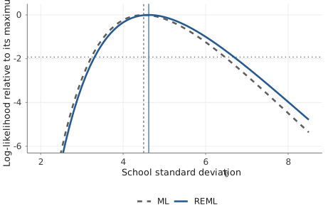
Note. NELS:88 subsample, random-intercept model for mathematics with homework. Curves: maximized log-likelihood (dashed, ML) and restricted log-likelihood (solid, REML) as functions of ${\tau }_0$, each relative to its maximum, with ${\sigma }^2$ (and, for ML, the fixed effects) maximized out. Vertical lines: the ML (dashed) and REML (solid) estimates. Dotted horizontal line: $-1.92$, the cutoff for 95% likelihood-ratio intervals.

B.3Restricted Maximum Likelihood#

The ML estimator of a variance is biased downward because it ignores the degrees of freedom used to estimate the fixed effects; in ordinary regression, ML divides the residual sum of squares by $N$ and REML by $N-p$ (Chapter 9). REML has two equivalent derivations (Harville, 1974; Patterson & Thompson, 1971).

Error contrasts. Choose an $N\times (N-p)$ matrix $\mathbf{K}$ of full column rank with ${\mathbf{K}}^{\prime }\mathbf{X}=0$. The transformed data ${\mathbf{K}}^{\prime }\mathbf{y}\sim \mathcal{N}(0,{\mathbf{K}}^{\prime }\mathbf{V}\mathbf{K})$ do not depend on $\mathbf{\gamma }$, and REML maximizes their likelihood. Two matrix identities show that the result does not depend on the choice of $\mathbf{K}$: for any such $\mathbf{K}$, $\mathbf{K}({\mathbf{K}}^{\prime }\mathbf{V}\mathbf{K}{)}^{-1}{\mathbf{K}}^{\prime }=\mathbf{P}$, the matrix of Appendix A (Section A.7), and $\log |{\mathbf{K}}^{\prime }\mathbf{V}\mathbf{K}|=\log |{\mathbf{K}}^{\prime }\mathbf{K}|+\log |\mathbf{V}|+\log |{\mathbf{X}}^{\prime }{\mathbf{V}}^{-1}\mathbf{X}|-\log |{\mathbf{X}}^{\prime }\mathbf{X}|$, so that different choices of $\mathbf{K}$ change the log-likelihood only by the constant $-\frac{1}{2}\log |{\mathbf{K}}^{\prime }\mathbf{K}|$. For $\mathbf{K}$ with orthonormal columns, $|{\mathbf{K}}^{\prime }\mathbf{K}|=1$, and therefore

where the last term does not involve $\mathbf{\theta }$ and is usually dropped by software; without it, the REML criterion changes when a predictor is rescaled (Chapter 10). For the NELS:88 data, the log-likelihood of ${\mathbf{K}}^{\prime }\mathbf{y}$ computed directly from a 519 $\times$ 517 orthonormal $\mathbf{K}$ differs from the formula without the constant by 6.65, which equals $\frac{1}{2}\log |{\mathbf{X}}^{\prime }\mathbf{X}|$, at every value of $\mathbf{\theta }$ tried (to within $10^{-11}$).

Integrated likelihood. The same function arises by integrating the likelihood over the fixed effects with a flat prior, $L_R(\mathbf{\theta })\propto \int L(\mathbf{\gamma },\mathbf{\theta })d\mathbf{\gamma }$ (Harville, 1974). Because $\ell (\mathbf{\gamma },\mathbf{\theta })$ is quadratic in $\mathbf{\gamma }$, $\ell (\mathbf{\gamma },\mathbf{\theta })={\ell }_p(\mathbf{\theta })-\frac{1}{2}(\mathbf{\gamma }-\hat{\mathbf{\gamma }}{)}^{\prime }{\mathbf{X}}^{\prime }{\mathbf{V}}^{-1}\mathbf{X}(\mathbf{\gamma }-\hat{\mathbf{\gamma }})$, and the integral of the exponential of the second term is $(2\pi {)}^{p/2}|{\mathbf{X}}^{\prime }{\mathbf{V}}^{-1}\mathbf{X}{|}^{-1/2}$. The factor $|{\mathbf{X}}^{\prime }{\mathbf{V}}^{-1}\mathbf{X}{|}^{-1/2}$ is the REML correction: it penalizes values of $\mathbf{\theta }$ under which the fixed effects are estimated precisely, which offsets the too-small residuals that arise when $\hat{\mathbf{\gamma }}$ is fitted to the same data. At $\hat{\mathbf{\gamma }}$, the quadratic form of Equation (B.3) equals ${\mathbf{y}}^{\prime }\mathbf{P}{\dot{\mathbf{V}}}_k\mathbf{P}\mathbf{y}$, where ${\dot{\mathbf{V}}}_k$ is block diagonal with blocks ${\dot{\mathbf{V}}}_{jk}$, and its expectation is $\mathrm{tr}(\mathbf{P}{\dot{\mathbf{V}}}_k)$, not $\mathrm{tr}({\mathbf{V}}^{-1}{\dot{\mathbf{V}}}_k)$. The REML score equations use this trace, so they equate the quadratic form with its expectation after $\mathbf{\gamma }$ has been estimated. REML estimates of the fixed effects are the GLS estimates at ${\hat{\mathbf{\theta }}}_{\mathrm{REML}}$. Because ${\ell }_R$ is the likelihood of the error contrasts ${\mathbf{K}}^{\prime }\mathbf{y}$, and $\mathbf{K}$ depends on $\mathbf{X}$, models with different fixed effects have REML likelihoods of different data, which cannot be compared (Chapters 9 and 10).

B.4Information and Standard Errors of Variance Components#

The expected information matrix of the linear mixed model is block diagonal: the ML estimators of the fixed effects and of the variance components are asymptotically independent. The block for $\mathbf{\gamma }$ is ${\sum }_j{\mathbf{X}}_j^{\prime }{\mathbf{V}}_j^{-1}{\mathbf{X}}_j$, whose inverse is the GLS covariance matrix, and the block for the variance components has elements

For the NELS:88 model at the ML estimates, the inverse of Equation (B.5) gives standard errors of 7.06 for ${\hat{\tau }}_0^2$ and 4.52 for ${\hat{\sigma }}^2$. The delta method (Appendix A, Section A.9) converts them into 0.79 for ${\hat{\tau }}_0$ and, for the residual intraclass correlation $\hat{\rho }=.22$, into a standard error of 0.062. Under REML, the elements of Equation (B.5) become $\frac{1}{2}\mathrm{tr}(\mathbf{P}{\dot{\mathbf{V}}}_k\mathbf{P}{\dot{\mathbf{V}}}_l)$, and many programs use the observed information, the negative Hessian, often computed numerically, in place of the expected information; the two agree in large samples. Large here means many clusters: the asymptotic results for the cluster-level parameters rest on a growing number of clusters $J$, and more observations per cluster do not substitute for more clusters. Wald intervals built from these standard errors assume a normal, symmetric sampling distribution; with 23 schools, the profile interval of Section B.2 is more trustworthy.

B.5Algorithms in Brief#

Newton–Raphson iterates ${\mathbf{\theta }}^{(t+1)}={\mathbf{\theta }}^{(t)}-{\mathbf{H}}^{-1}\mathbf{s}$ with the score $\mathbf{s}$ and the Hessian $\mathbf{H}$ of the log-likelihood; Fisher scoring replaces $-\mathbf{H}$ by the expected information (B.5), which is easier to compute and positive definite whenever the variance components are identified, whereas $-\mathbf{H}$ need not be positive definite far from the maximum; Fisher scoring is therefore often more stable in early iterations. Goldstein’s iterative generalized least squares alternates GLS for $\mathbf{\gamma }$ with a GLS regression of the squared and cross-product residuals on the design of $\mathbf{V}$ (Goldstein, 1986). The EM algorithm treats the random effects as missing data (Dempster et al., 1977; Laird & Ware, 1982): the E-step computes $E({\mathbf{u}}_j\mid {\mathbf{y}}_j)$ and $\mathrm{Var}({\mathbf{u}}_j\mid {\mathbf{y}}_j)$ at the current parameters (Section B.6), and the M-step updates $\mathbf{T}$ to the average of $E({\mathbf{u}}_j{\mathbf{u}}_j^{\prime }\mid {\mathbf{y}}_j)$, ${\sigma }^2$ to the average expected squared level-1 residual, and $\mathbf{\gamma }$ by least squares applied to ${\mathbf{y}}_j-{\mathbf{Z}}_{j}E({\mathbf{u}}_j\mid {\mathbf{y}}_j)$ (Chapter 9) or, in a common variant, by GLS. EM never decreases the likelihood but converges slowly near the maximum, and Lindstrom & Bates (1988) concluded that a well-implemented Newton–Raphson algorithm is preferable in most situations. lme4 minimizes the profiled deviance over the elements of ${\mathbf{\Lambda }}_{\mathbf{\theta }}$ with derivative-free bounded optimizers, using sparse Cholesky factorizations (Bates et al., 2015); Chapter 9 runs Newton–Raphson, Fisher scoring, and EM on the NELS:88 empty model (Table 9.3) and discusses estimation problems and their remedies.

B.6Empirical Bayes Prediction, BLUP, and Henderson’s Equations#

The posterior of the random effects. Treating ${\mathbf{u}}_j\sim \mathcal{N}(0,\mathbf{T})$ as a prior and ${\mathbf{y}}_j\mid {\mathbf{u}}_j\sim \mathcal{N}({\mathbf{X}}_j\mathbf{\gamma }+{\mathbf{Z}}_j{\mathbf{u}}_j,{\sigma }^2\mathbf{I})$ as the likelihood, Bayes’ theorem gives a normal posterior, because the exponent of the product of the two densities is quadratic in ${\mathbf{u}}_j$. Collecting the quadratic and linear terms,

By the Woodbury identity (Appendix A, Section A.5), the mean equals $\mathbf{T}{\mathbf{Z}}_j^{\prime }{\mathbf{V}}_j^{-1}({\mathbf{y}}_j-{\mathbf{X}}_j\mathbf{\gamma })$ and the variance equals $\mathbf{T}-\mathbf{T}{\mathbf{Z}}_j^{\prime }{\mathbf{V}}_j^{-1}{\mathbf{Z}}_j\mathbf{T}$, the conditional-normal results of Appendix A (Section A.8). Replacing $\mathbf{\gamma }$ and $\mathbf{\theta }$ by estimates gives the empirical Bayes predictions of Chapter 12. For the random intercept, the posterior mean is the shrinkage estimator ${\lambda }_j({\bar{y}}_j-{\bar{\mathbf{x}}}_j^{\prime }\mathbf{\gamma })$ with ${\lambda }_j=n_j{\tau }_0^2/({\sigma }^2+n_j{\tau }_0^2)$.

BLUP and the mixed-model equations. Without the normality assumption, the posterior mean with $\mathbf{\gamma }$ replaced by its GLS estimate, $\mathbf{T}{\mathbf{Z}}_j^{\prime }{\mathbf{V}}_j^{-1}({\mathbf{y}}_j-{\mathbf{X}}_j\hat{\mathbf{\gamma }})$, is the best linear unbiased predictor (BLUP) when $\mathbf{\theta }$ is known: among linear functions of $\mathbf{y}$ whose prediction errors have mean zero for every $\mathbf{\gamma }$, it minimizes the mean squared prediction error (Henderson, 1975; Robinson, 1991). With estimated $\mathbf{\theta }$, it is the empirical BLUP (Chapter 12). Henderson obtained the estimates of $\mathbf{\gamma }$ and the predictions of $\mathbf{u}=({\mathbf{u}}_1^{\prime },\dots ,{\mathbf{u}}_J^{\prime }{)}^{\prime }$ jointly by maximizing the joint density of $\mathbf{y}$ and $\mathbf{u}$, which is equivalent to minimizing the penalized sum of squares ${\sigma }^{-2}\Vert \mathbf{y}-\mathbf{X}\mathbf{\gamma }-\mathbf{Z}\mathbf{u}{\Vert }^2+{\mathbf{u}}^{\prime }{\mathbf{G}}^{-1}\mathbf{u}$ with $\mathbf{G}={\mathbf{I}}_J\otimes \mathbf{T}$ and $\mathbf{Z}=\mathrm{diag}({\mathbf{Z}}_1,\dots ,{\mathbf{Z}}_J)$. Setting the derivatives to zero gives the mixed-model equations

Solving the second block for $\hat{\mathbf{u}}=({\mathbf{Z}}^{\prime }\mathbf{Z}+{\sigma }^2{\mathbf{G}}^{-1}{)}^{-1}{\mathbf{Z}}^{\prime }(\mathbf{y}-\mathbf{X}\hat{\mathbf{\gamma }})$ and substituting into the first gives ${\mathbf{X}}^{\prime }{\mathbf{V}}^{-1}\mathbf{X}\hat{\mathbf{\gamma }}={\mathbf{X}}^{\prime }{\mathbf{V}}^{-1}\mathbf{y}$ by the Woodbury identity (Appendix A, Section A.5), so $\hat{\mathbf{\gamma }}$ is the GLS estimator, and $\hat{\mathbf{u}}$ is the posterior mean (B.6) evaluated at $\hat{\mathbf{\gamma }}$. Multiplied by ${\sigma }^2$, the penalty is, for a random intercept, $({\sigma }^2/{\tau }_0^2){\sum }_j{u}_j^2$, the ridge penalty of Chapter 32 with penalty parameter ${\sigma }^2/{\tau }_0^2$. The inverse of the coefficient matrix in Equation (B.7) contains the covariance matrix of $\hat{\mathbf{\gamma }}$ in its upper-left block and, in its lower-right block, the prediction error variances $\mathrm{Var}(\hat{\mathbf{u}}-\mathbf{u})$, which, unlike the posterior variances of Equation (B.6), include the uncertainty of $\hat{\mathbf{\gamma }}$.

For the NELS:88 model with the REML variance components, the solution of Equation (B.7) equals the lme4 fixed effects, their covariance matrix, and the predicted school effects to within $10^{-12}$. For the smallest school ($n_j=5$), the posterior standard deviation reported by lme4 is 2.92 and the prediction error standard deviation is 2.99; for the largest school ($n_j=67$), they are 1.01 and 1.47. For a random intercept, the uncertainty of $\hat{\mathbf{\gamma }}$ adds ${\lambda }_j^2{\bar{\mathbf{x}}}_j^{\prime }\mathrm{Var}(\hat{\mathbf{\gamma }}){\bar{\mathbf{x}}}_j$ to the posterior variance, and this addition tends to be largest for the schools whose own data determine their effect most precisely, because their predictions are shrunken least.

B.7Generalized Linear Mixed Models: Laplace, Quadrature, and PQL#

For a GLMM, the conditional distribution of ${\mathbf{y}}_j$ given ${\mathbf{u}}_j$ is, for example, Bernoulli, binomial, or Poisson, and the marginal likelihood of cluster $j$,

has no closed form. Three approximations are in common use (Chapter 23).

Laplace approximation. Expand $h_j$ to second order around its maximum ${\hat{\mathbf{u}}}_j$, the conditional mode: $h_j(\mathbf{u})\approx h_j({\hat{\mathbf{u}}}_j)-\frac{1}{2}(\mathbf{u}-{\hat{\mathbf{u}}}_j{)}^{\prime }{\mathbf{H}}_j(\mathbf{u}-{\hat{\mathbf{u}}}_j)$ with ${\mathbf{H}}_j=-{\partial }^2{h}_j/\partial \mathbf{u}\partial {\mathbf{u}}^{\prime }$ at ${\hat{\mathbf{u}}}_j$. The remaining integral is a normal integral, so that, with $q$ the dimension of ${\mathbf{u}}_j$,

The approximation is exact when the integrand is proportional to a normal density and deteriorates when it is skewed, as it is with few binary observations per cluster; its asymptotic bias is larger for binary and ordinal than for count responses and decreases as the cluster size grows (Joe, 2008).

Adaptive Gauss–Hermite quadrature. Quadrature replaces the integral by a weighted sum over $Q$ nodes. Nonadaptive quadrature uses the same nodes for every cluster, such as the fixed grid of mirt (Chapter 30), and needs many of them. Adaptive quadrature centers the nodes at ${\hat{\mathbf{u}}}_j$ and scales them by $\sqrt{2}{\mathbf{H}}_j^{-1/2}$, so that they fall where the integrand has its mass; with a single node it reduces to the Laplace approximation, and the error decreases rapidly as $Q$ grows (Pinheiro & Bates, 1995; Rabe-Hesketh et al., 2002). The number of function evaluations grows as $Q^q$ with the dimension $q$ of ${\mathbf{u}}_j$, and glmer offers quadrature only for models with a single scalar random-effects term.

Penalized quasi-likelihood. PQL linearizes the model around the current predictions and fits a linear mixed model to a working response, iterating to convergence (Breslow & Clayton, 1993). It is fast and extends to complex random-effects structures, but with binary outcomes, small clusters, and a large variance, it underestimates variance components and attenuates the fixed effects on the logit scale toward zero, as Rodríguez & Goldman (1995) showed for the closely related MQL and Rodríguez & Goldman (2001) for PQL, and as the simulation of Chapter 23 confirms.

Example. Figure B.2 shows $\exp \{h_j(u)-h_j({\hat{u}}_j)\}$ for district 41 of the contraception data (26 women, 13 of them using contraception), the district whose likelihood contribution the Laplace approximation reproduces least well. Even here the two curves cannot be told apart, so the figure shows how the approximation works, not how it fails: the Laplace error for this district is 0.3% (median over districts 0.2%), and five adaptive quadrature nodes reduce it below $10^{-6}$ in relative terms. Table B.1 compares the approximations for the whole model. The Laplace $-2\log L$ exceeds the 25-node quadrature value by 0.27, almost all of it approximation error rather than a difference in fit (likelihoods from different approximations should therefore not be compared; Chapters 23 and 24), and the district standard deviation moves from 0.474 to 0.477; three nodes come within 0.02 of the converged $-2\log L$, and from seven nodes on nothing changes at the precision shown. PQL gives a smaller standard deviation (0.464) and a smaller urban coefficient (0.681 against 0.692), in the direction of its known bias. With districts of median size 26 and a small variance, as here, the Laplace approximation is adequate. With five binary items per person, it underestimated the person standard deviation of a simulated Rasch model by about 5% (Chapter 30), and with clusters of two, it underestimated the variance by 26% to 33% for true variances from 0.5 to 5 (Chapter 23).

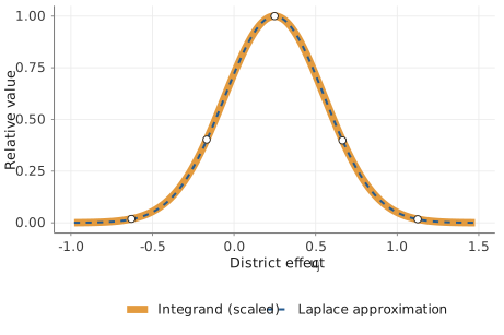
Note. Thick light line: $\exp \{h_j(u)-h_j({\hat{u}}_j)\}$, the integrand of Equation (B.8) divided by its maximum, for one district, evaluated at the Laplace estimates of the fixed effects and the district variance; thin dashed line: the normal curve of the Laplace approximation, with the same mode and curvature. Circles: the five nodes of adaptive Gauss–Hermite quadrature.

B.8Likelihood-Ratio Tests on the Boundary#

The usual chi-square distribution of the likelihood-ratio statistic rests on a quadratic approximation of the log-likelihood around a true value in the interior of the parameter space. When the null hypothesis sets a variance to zero, the true value is on the boundary, and the estimator is constrained to be nonnegative. In large samples, the unconstrained estimate is approximately normal around zero; with probability one half it is negative, the constrained estimate is zero, and the likelihood-ratio statistic is zero; with probability one half it is positive, and the statistic is the square of an approximately standard normal variable. This heuristic, which assumes a single parameter on the boundary with all others in the interior, gives the 50:50 mixture of ${\chi }_0^2$ and ${\chi }_1^2$ (Self & Liang, 1987; Stram & Lee, 1994). Testing a random slope that is correlated with the intercept, whose variance and covariance with the intercept both vanish under the null hypothesis, leads instead to the 50:50 mixture of ${\chi }_1^2$ and ${\chi }_2^2$; critical values and further cases are given in Appendix A (Section A.12) and applied in Chapter 11. The asymptotic argument again rests on the number of clusters; in finite samples the mixture tends to be conservative, and a parametric bootstrap of the likelihood-ratio statistic, or, for a model with a single variance component, its exact null distribution (Crainiceanu & Ruppert, 2004), is safer (Chapter 11).

Further Reading#

Harville (1977); Searle et al. (1992)

ML and REML estimation of variance components.

Robinson (1991)

BLUP, Henderson’s equations, and their many interpretations.

Pinheiro & Bates (1995); Rabe-Hesketh et al. (2002)

The Laplace approximation and adaptive quadrature.

Verbeke & Molenberghs (2000)

The linear mixed model for longitudinal data, with derivations.