Multilevel Data, Multilevel Questions
In this chapterwhy nested data need their own models; how multilevel data arise; how dependence changes inference; how multilevel questions are stated; what the rest of the book covers.
Suppose a researcher wants to know whether pupils who spend more time on mathematics homework obtain higher mathematics scores. The data come from a national survey in which schools were sampled first and pupils were then sampled within each school. The researcher runs an ordinary regression of mathematics score on homework time using all pupils, obtains a large and highly significant slope, and writes it up. A reviewer returns the paper with three questions. Are pupils in the same school really independent observations? Is the slope a statement about pupils, about schools, or a mixture of both? And could the answer differ from school to school? This chapter is about why these three questions arise whenever data have a nested structure, and why they are not technicalities but part of the substance of the research question.
1.1What Multilevel Analysis Is#
Snijders & Bosker (2012) describe multilevel analysis as a methodology for data whose variability has a complex pattern, with a particular focus on sources of variability that are nested within one another. Pupils vary around the mean of their class, classes vary around the mean of their school, and schools vary around the mean of the population. Each of these sources of variation can be of interest in its own right, and each can be related to explanatory variables measured at the corresponding level. A multilevel model is a statistical model that represents all of these sources of variation at once, together with the explanatory variables that are thought to account for them.
Multilevel models were developed in several disciplines at roughly the same time, and they carry several names (Table 1.1). In education and psychology the most common names are hierarchical linear model (Raudenbush & Bryk, 2002) and multilevel model (Goldstein, 2011; Hox et al., 2018; Snijders & Bosker, 2012). In statistics and biostatistics the same models are called linear mixed models or mixed-effects models (Laird & Ware, 1982; Verbeke & Molenberghs, 2000), because they combine fixed effects, which are constant across groups, with random effects, which vary across groups. Other names are random coefficient models (Longford, 1993), variance components models (Searle et al., 1992), growth curve models for longitudinal data (Singer & Willett, 2003), and hierarchical Bayesian models (Gelman & Hill, 2007). The names differ in what they emphasize, but for continuous outcomes they refer to one family of models; the hierarchical Bayesian version adds prior distributions for the parameters and is estimated by Bayesian methods (Chapter 13). The generalized linear mixed model extends the same family to binary, ordinal, and count outcomes and is the subject of Part VI of this book.
| Name | What the name emphasizes | Typical fields |
|---|---|---|
| Hierarchical linear model (HLM) | Separate equations for each level of a nested structure | Education, psychology |
| Multilevel model | Variables and variation at several levels | Education, sociology, psychology |
| Linear mixed (effects) model | A single equation with fixed and random effects | Statistics, biostatistics, linguistics |
| Random coefficient model | Regression coefficients that vary over groups | Statistics, economics |
| Variance components model | Partitioning outcome variance into level-specific parts | Statistics, genetics, measurement |
| Growth curve model | Person-specific trajectories over time | Developmental and clinical psychology |
| Hierarchical Bayesian model | Parameters that follow a distribution with its own parameters | Statistics, cognitive science |
| Generalized linear mixed model (GLMM) | Random effects in models for binary, ordinal, or count outcomes | All of the above |
Note. The names overlap; for continuous outcomes they refer to one family of models written in different ways (see Chapter 2).
This book uses the terms multilevel model, hierarchical linear model, and linear mixed model interchangeably, and it chooses among them according to which way of writing the model is most helpful at a given point. Chapter 2 shows that one model can be written in three equivalent ways (as a set of level-specific equations, as a single mixed-model equation, and as a marginal model for the mean and covariance of the outcome), and that moving among the three ways is the key to reading the output of any software package.
1.2Hierarchies Everywhere#
1.2.1Examples of nested data#
Data in psychology, education, health, and the social sciences are very often grouped. Pupils are taught in classes, and classes belong to schools. Patients are treated by therapists, who work in clinics. Employees work in teams within firms. Survey respondents are interviewed by interviewers and live in households within sampling areas. Table 1.2 lists examples from several fields. In each row, the units in one column are nested within the units in the next column, except where the table marks a classification as crossed.
| Field | Level 1 | Level 2 | Level 3 (if any) |
|---|---|---|---|
| Education | Pupils | Classes | Schools |
| Developmental psychology | Children | Families | Neighborhoods |
| Clinical psychology | Patients | Therapists | Clinics |
| Organizational psychology | Employees | Work teams | Firms |
| Survey research | Respondents | Interviewers or households | Sampling areas |
| Longitudinal research | Measurement occasions | Persons | Groups (e.g., schools) |
| Experience sampling | Daily or momentary reports | Persons | Couples or families |
| Experimental psychology | Trials | Participants (crossed with stimuli) | Laboratories |
| Measurement | Item responses | Persons (crossed with items) | Schools or countries |
| Meta-analysis | Study participants | Studies | Research groups |
| Cross-national research | Individuals | Country-by-year surveys | Countries |
Note. Each row lists units from the lowest level (level 1) to higher levels. “Crossed with” marks a second classification that is not nested in the first (see Figure 1.1).
Two entries in the table deserve comment. First, repeated measurements on the same persons also form a hierarchy: measurement occasions (level 1) are nested within persons (level 2). Longitudinal and repeated-measures data are therefore multilevel data, and much of the modern analysis of change is multilevel analysis (Hoffman, 2015; Singer & Willett, 2003). Second, some structures are not strictly nested. In a reaction-time experiment in which every participant responds to every stimulus, trials are classified both by participant and by stimulus, and neither classification is nested in the other (Baayen et al., 2008; Judd et al., 2012).
1.2.2Five data structures#
Figure 1.1 draws five common structures as unit diagrams, in which each box or circle is one unit and each line means “belongs to” (see also Browne et al., 2001). In a two-level structure (panel a) every pupil belongs to exactly one school. In a three-level structure (panel b) pupils belong to classes and classes belong to schools. In a repeated-measures or longitudinal structure (panel c) occasions belong to persons, and persons may be observed on different numbers of occasions. In a cross-classified structure (panel d) pupils belong to a neighborhood and to a school, and because pupils from one neighborhood attend different schools and each school draws pupils from several neighborhoods, neither classification is nested in the other (Rasbash & Goldstein, 1994). In a multiple-membership structure (panel e) some pupils belong to more than one school, for example because they changed schools during the year, and each membership receives a weight.
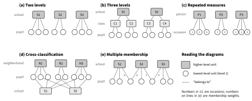
Note. Dark-shaded rectangles represent higher-level units, light-shaded rectangles represent intermediate-level units (panel b) or a second classification (panel d), and circles represent level-1 units. A line joins a unit to each unit it belongs to. Numbers inside circles in panel (c) index occasions; numbers on lines in panel (e) are membership weights.
Parts II to V of this book deal mainly with the nested structures in panels (a) to (c). Cross-classified and multiple-membership structures are treated in Chapter 26, and crossed designs with persons and items return in the measurement chapter (Chapter 30).
1.2.3Levels, units, and terminology#
The level of a unit is its position in the hierarchy. By convention the lowest level, where the outcome is usually measured, is level 1. Units at level 1 are also called micro-level units, elementary units, or individuals; units at level 2 are called macro-level units, clusters, or groups. This book mostly uses level-1 unit and cluster (or the substantive name, such as pupil and school), and uses group as a neutral word when the kind of cluster does not matter. The number of level-2 units is written , the number of level-1 units in cluster is written , and the total number of level-1 units is .
A variable also has a level: the level of the units on which it is measured. Mathematics score and homework time are pupil-level (level-1) variables. School sector (public or private) and pupil–teacher ratio are school-level (level-2) variables. A school-level variable can also be constructed from pupil data by aggregation; the mean socioeconomic status of the pupils in a school is a school-level variable, even though it is computed from pupil-level scores. Conversely, a school-level variable is often attached to every pupil in the data file (by disaggregation), so the same value appears on many rows. A column that varies within clusters is a level-1 variable, but a column that is constant within clusters may be either a level-2 variable or a level-1 variable that happens not to vary in these data; the level of a variable follows from the design and from the definition of the variable, not from the pattern of values in the file.
1.2.4Where variables live: a first look at plates#
This book draws every model with one graphical grammar, the Unified Model Graph (UMG; Yu, 2026a, 2026b), which is introduced fully in Chapter 2. One element of that grammar is useful from the start. A plate is a rounded box that means “repeated for every unit at this level” (Buntine, 1994). Plates are nested when units are nested. A variable is drawn inside every plate whose index it carries and outside every other plate.
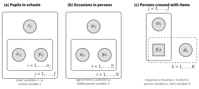
Note. Shaded circles represent observed continuous variables; the shaded square in panel (c) represents an observed categorical response. Rounded boxes (plates) mean “repeated for every unit at this level,” with the index range printed in a corner. Plates drawn inside other plates represent nesting; the overlapping solid and dashed plates in panel (c) represent crossing. No arrows are drawn because no model has yet been specified.
Figure 1.2 shows three examples. In panel (a) the pupil plate () sits inside the school plate (). The pupil variables and are inside the pupil plate because they take a different value for every pupil; the school variable is inside the school plate but outside the pupil plate because it takes one value per school. In panel (b) occasions () are nested in persons (): age or time and the outcome change from occasion to occasion, whereas a stable characteristic such as sex, , does not. In panel (c) persons and items are crossed: the response lies where the person plate and the item plate overlap, because there is one response for each combination of person and item, while person variables such as and item variables such as lie in only one of the two plates. The subscripts in the equations and the plates in the figure carry the same information. A reader who can place every variable of a study in the correct plate has already understood most of what distinguishes a multilevel analysis from an ordinary one.
1.3Why Members of a Group Resemble Each Other#
Children with the same biological parents tend to be more alike than children chosen at random from the population. They are more alike because they share genes, because they share an environment, and usually because of both. The same is true, for different reasons, of pupils in the same school. Pupils in one school share the same school environment and often the same teachers; they influence each other through direct contact and shared norms; and they tend to come from the same neighborhood, so they were already similar before they entered the school. In general, members of a group resemble each other for four kinds of reasons: they share a common context (school resources, a therapist’s skill, a manager’s style); they were selected into the group in ways that depend on their characteristics (families choose neighborhoods and schools; patients choose clinics); they interact and influence one another (contagion, norms, competition); and they are measured in a common way (the same interviewer, the same rater, the same test administration).
The consequence is the same whatever the mechanism: observations in the same group are statistically dependent. Knowing the score of one pupil tells us something about the likely score of another pupil in the same school, beyond what the population mean tells us. Table 1.3 makes the idea concrete with a simple measurement, blood pressure, taken under four designs. As the design moves from unrelated persons (Design I) to repeated measurements on members of many families (Design IV), new sources of variability are added, and each new source that several measurements share introduces a new kind of dependence among the measurements.
| Design | Measurements of blood pressure taken … | Sources of variability |
|---|---|---|
| I | once on each of many unrelated persons | Measurement error; differences between persons |
| II | once on each member of many families | Measurement error; differences between members; differences between families |
| III | repeatedly on each person, over time or conditions | Measurement error; serial (time-related) variation; differences between persons |
| IV | repeatedly on each member of many families | Measurement error; serial variation; differences between members; differences between families |
Note. Designs II and III each add a source of variability to Design I, and Design IV combines both additions. Every added source that is shared by several measurements creates dependence among those measurements.
Dependence is sometimes treated as a nuisance: a violation of the independence assumption that must be “corrected.” It is more useful to treat it as information. The amount of variation that lies between schools, and the way it changes when explanatory variables are added, tells us how much outcomes differ between schools and which variables account for those differences. The variation between persons in repeated-measures data tells us how stable individual differences are. In many studies the dependence is itself the phenomenon of interest.
1.4How Multilevel Data Arise#
The structure of a data set follows from the way the data were collected. Two broad routes lead to multilevel data: observational studies with multistage sampling, and experiments in which groups are formed or assigned.
1.4.1Observational studies and multistage sampling#
Large surveys rarely draw a simple random sample of individuals. It is much cheaper to draw a random sample of schools, then a random sample of classes within each sampled school, and then pupils within each sampled class. Such multistage (or cluster) sampling is cost-effective, but it produces data in which the primary sampling units are clusters (Kish, 1965). The usual assumptions of a multilevel analysis mirror the sampling design: the level-2 units are a random (or at least representative) sample from a population of level-2 units, and within each sampled level-2 unit the level-1 units are a random (or representative) sample from that unit. When these assumptions hold approximately, the variation among sampled schools estimates the variation among schools in the population, and inferences can be made about schools in general and not only about the schools in the sample.
Many of the data sets used in this book come from designs of this kind. The National Education Longitudinal Study of 1988 (NELS:88) sampled schools and then eighth-grade students within schools; the High School and Beyond survey used in Chapter 5 has the same structure; international assessments such as PISA sample schools and then students within schools, and TIMSS samples schools and then intact classes within schools. In each case the analysis must respect the stages of the sample.
1.4.2Experiments#
Hierarchies are also created by experiments. When patients are randomly assigned to clinics, or pupils to classes, the random assignment ensures that the groups do not differ systematically at the outset, but it does not make the members of a group independent afterward. Patients treated in the same clinic share the same staff and procedures; pupils in the same class share the same teacher and influence one another. Grouping may be random at the start of a study, and yet over the course of the study the groups become differentiated, because the group affects its members and the members affect the group.
When whole groups (schools, clinics, communities) are randomly assigned to conditions, the design is a cluster-randomized or group-randomized trial (Murray, 1998; Raudenbush, 1997). The treatment then varies only between clusters, and, as Section 1.6 shows, the number of clusters, more than the number of individuals, determines how much information the study has about the treatment effect.
1.4.3Longitudinal, intensive, and crossed designs#
In longitudinal studies the same persons are measured repeatedly, so occasions are nested within persons. Traditional repeated-measures analysis of variance requires a balanced design: the same occasions for all persons and no missing data. A multilevel analysis allows persons to be measured at different times and on different numbers of occasions, can include explanatory variables that change over time, and can model how the residuals of one person are correlated over time (Hedeker & Gibbons, 2006; Singer & Willett, 2003). Diary and experience-sampling studies, in which persons report their mood or behavior several times a day over several weeks, produce dozens or hundreds of occasions per person and are analyzed with the same models (Bolger & Laurenceau, 2013). In experimental psychology, designs in which each participant responds to many stimuli produce trials classified by both participant and stimulus, and treating stimuli as a random factor is necessary whenever the conclusions are meant to generalize to other stimuli (Judd et al., 2012).
1.5A First Look at Multilevel Data#
1.5.1Two schools from NELS:88#
NELS:88 was conducted by the National Center for Education Statistics of the U.S. Department of Education. Its first wave, collected in the spring of 1988, measured about 25,000 eighth-grade students in about 1,000 schools. Kreft & de Leeuw (1998) made available a subsample of 23 schools with 519 students, which this book uses repeatedly (the data are described in Appendix C). The outcome is a mathematics test score, and one pupil-level explanatory variable is the time a pupil reports spending on mathematics homework each week, recorded in eight ordered categories from “none” to “10 or more hours.”
Figure 1.3 plots mathematics score against homework time for two of the 23 schools, and Table 1.4 summarizes them. School 24725 is a public school whose pupils have below-average socioeconomic status (SES); school 62821 is a private school whose pupils have well-above-average SES. The two schools differ in almost every respect. Their mean mathematics scores differ by about 19 points. Pupils in the private school report more homework (a mean category code of 3.3 versus 1.6; the codes are ordered categories, not hours). The spread of scores is larger in the public school. Most importantly for the question that opened the chapter, the relation between homework and mathematics differs: the least-squares slope is about 5.6 points per homework category in the public school and about 1.1 points in the private school.
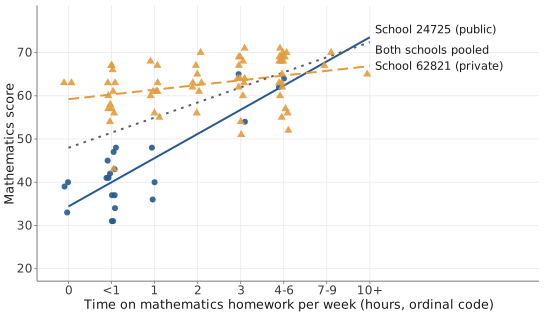
Note. Circles and the solid line represent pupils and the least-squares line for school 24725; triangles and the dashed line represent pupils and the line for school 62821; the dotted line is the least-squares line for the two schools pooled. Points are jittered horizontally to reduce overlap. Homework is recorded in ordered categories; tick labels give the hours per week that each category represents.
| Mathematics | Within-school OLS | ||||||
|---|---|---|---|---|---|---|---|
| School | Mean | SD | Homework | SES | Intercept | Slope | |
| 24725 (public) | 22 | 43.5 | 10.0 | 1.64 | 0.70 | 34.4 | 5.59 |
| 62821 (private) | 67 | 62.8 | 5.7 | 3.30 | 1.04 | 59.2 | 1.09 |
| Pooled (both schools) | 89 | 58.1 | 10.9 | 2.89 | 0.61 | 48.0 | 3.49 |
Note. = number of pupils; Homework = mean of the eight-category homework code (0–7); SES = mean standardized socioeconomic status; Intercept and Slope = ordinary least-squares (OLS) regression of mathematics on the homework code.
If the pupils of the two schools are pooled and a single regression line is fitted, the slope is about 3.5. This pooled slope describes neither school. It mixes the relation between homework and mathematics within schools with the difference between schools, which differ in both homework and mathematics for reasons that may have little to do with homework itself (sector, SES, and whatever else distinguishes the two schools). This small example already raises all three of the reviewer’s questions from the start of the chapter.
1.5.2Fifty schools from the Junior School Project#
The Junior School Project (JSP; Mortimore et al., 1988) followed nearly 2,000 pupils in 50 inner-London primary schools through the four junior-school years (1980–1984), and its data have been used to illustrate multilevel models since Goldstein (1987). The widely distributed version used here contains test scores from three of those years: 3,236 records on 1,192 pupils in 49 schools, of whom 1,093 have mathematics scores in both year 0 and year 1.
Figure 1.4 shows two views of the relation between mathematics in year 0 and mathematics in year 1. Panel (a) shows the pupils of one school (school 1). The relation is strong ( for the 32 pupils) and approximately linear. Panel (b) shows the least-squares line for each of the 49 schools, drawn over the range of year-0 scores observed in that school. About 80% of the within-school values lie between .35 and .82 (the 10th and 90th percentiles), so in most schools prior achievement predicts later achievement well. The lines, however, are not identical: they differ in height (pupils with the same year-0 score tend to score higher in year 1 in some schools than in others) and in slope (the median slope is 0.85, but slopes range from near zero to 1.3). The first kind of difference is the concern of school-effectiveness research: which schools do better than expected given their intake (Aitkin & Longford, 1986)? The second kind of difference asks whether schools are equally effective for pupils with low and high prior achievement.
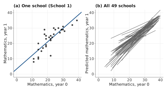
Note. Panel (a): points represent the pupils of school 1 and the line is their least-squares line. Panel (b): each line segment is the least-squares line of one school, drawn over the range of year-0 scores observed in that school. Both axes use the 0–40 scale of the test.
With two schools, or even with five, separate regressions for each school are a sensible way to describe the data, and they are the right analysis if the only interest is in those particular schools. With 49 schools, however, the separate regressions, which are noisiest in the smallest schools, do not answer the questions a researcher usually asks: How much do schools differ in general? Which school characteristics explain the differences? How confident can we be about the effect of a particular school, given how few pupils it contributed? Once the schools are regarded as a sample from a larger population of schools, these questions call for a model in which the school-specific intercepts and slopes are themselves random quantities with a distribution. That model is the multilevel model, and the random intercept and random slope versions of it are the subjects of Chapters 5 and 6.
1.6Dependence and Its Consequences#
1.6.1The intraclass correlation#
The simplest way to describe dependence in nested data is to divide the variance of the outcome into two parts. Write the score of pupil in school as the sum of an overall mean , a school effect , and a pupil-level residual :
with and independent of each other. The between-school variance measures how much the schools’ true means vary around the overall mean, and the within-school variance measures how much pupils differ from the mean of their own school. Equation (1.1) is the empty (or null, or unconditional) multilevel model; it is the one-way random-effects analysis of variance model studied in Chapter 3 and the starting point of Chapter 5.
The intraclass correlation (ICC) is the proportion of the total variance that lies between clusters:
The ICC has two readings that are worth keeping apart. It is the proportion of variance in the outcome that is due to differences between clusters, and it is also the correlation between the outcomes of two different level-1 units drawn at random from the same cluster. Both readings follow from Equation (1.1): two pupils in school share the term , so their covariance is ; because each score has variance , their correlation is .
For the 23 NELS:88 schools, the empty model gives estimates and , so the estimated ICC is . About a quarter of the variance in mathematics scores lies between schools; equivalently, the scores of two pupils from the same school correlate about .24. For achievement outcomes in national samples of U.S. schools, unconditional ICCs between about .15 and .25 are typical, and smaller values occur in more homogeneous samples of schools (Hedges & Hedberg, 2007). In repeated-measures data the ICC is often much larger, because stable differences between persons account for a large share of the variance.
1.6.2The design effect and the effective sample size#
Dependence reduces the amount of independent information in the data. If pupils within a school were perfect copies of each other (), a school with 25 pupils would contribute no more information about the population mean than a single pupil. If pupils were completely independent (), the school would contribute 25 independent observations. For values in between, the loss of information is summarized by the design effect (Kish, 1965). For clusters of equal size ,
and the effective sample size is . The design effect is the factor by which the sampling variance of a mean is larger under cluster sampling than under simple random sampling of the same number of individuals (see the Technical Detail box below). For NELS:88, with the average cluster size of 22.6 pupils and the ICC to three decimals, .243, the design effect is about (an approximation, because the schools differ in size), so the 519 pupils carry about as much information about the overall mean as independently sampled pupils would.
1.6.3What happens to significance tests#
Ordinary least-squares (OLS) regression, the test, and analysis of variance all assume that observations are independent. When the data are clustered and this assumption is ignored, the formulas treat the observations as if they were independent pieces of information. For predictors that are themselves clustered, and above all for cluster-level predictors, the estimated standard errors are then too small, confidence intervals are too narrow, and null hypotheses are rejected too often (Barcikowski, 1981; Kenny & Judd, 1986).
Figure 1.5 and Table 1.5 show the size of the problem in a small simulation (the script, with its seeds and all replication-level results, is in the book’s repository; see the Lab section at the end of the chapter). Forty clusters were generated, half assigned to a “treatment” and half to a “control” condition, as in a cluster-randomized trial. The true treatment effect was zero, so every significant result is a Type I error. The outcome ICC was set to 0, .05, .10, or .20, and the cluster size to 5, 10, 25, or 50. Each condition was replicated 5,000 times, and each data set was analyzed in two ways: by an OLS test on all individuals, which ignores clustering, and by a test on the 40 cluster means, which respects it (with equal cluster sizes this cluster-level test, with degrees of freedom, is identical to the REML test of the treatment effect with the same degrees of freedom in a random intercept model, Chapter 5, whenever the estimated between-cluster variance is positive).
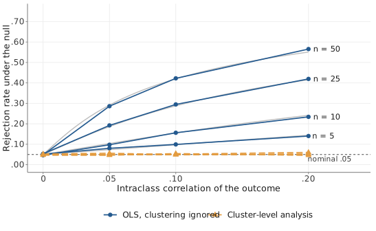
Note. Solid lines with circles show the rejection rate of the ordinary least-squares test that ignores clustering, for cluster sizes of 5, 10, 25, and 50 (labels at the right). Dashed lines with triangles show the rejection rate of the test on cluster means for the same cluster sizes; the four dashed lines nearly coincide. Thin gray curves show the rate predicted from the design effect. The dotted horizontal line marks the nominal .05 level. Each point is based on 5,000 replications with 40 clusters.
| Type I error rate () | |||||
|---|---|---|---|---|---|
| ICC | Design effect | Predicted (OLS) | OLS | Cluster-level | |
| .00 | 5 | 1.00 | .050 | .051 | .052 |
| .00 | 10 | 1.00 | .050 | .046 | .046 |
| .00 | 25 | 1.00 | .050 | .053 | .050 |
| .00 | 50 | 1.00 | .050 | .048 | .049 |
| .05 | 5 | 1.20 | .074 | .080 | .056 |
| .05 | 10 | 1.45 | .104 | .098 | .046 |
| .05 | 25 | 2.20 | .186 | .192 | .050 |
| .05 | 50 | 3.45 | .291 | .286 | .049 |
| .10 | 5 | 1.40 | .098 | .099 | .049 |
| .10 | 10 | 1.90 | .155 | .156 | .054 |
| .10 | 25 | 3.40 | .288 | .295 | .052 |
| .10 | 50 | 5.90 | .420 | .422 | .049 |
| .20 | 5 | 1.80 | .144 | .140 | .050 |
| .20 | 10 | 2.80 | .241 | .234 | .046 |
| .20 | 25 | 5.80 | .416 | .420 | .060 |
| .20 | 50 | 10.80 | .551 | .566 | .053 |
Note. ICC = intraclass correlation of the outcome; = cluster size (40 clusters in every condition); Design effect ; Predicted (OLS) = two-sided rejection rate implied by the design effect, ; OLS = test on individuals ignoring clustering; Cluster-level = test on the 40 cluster means. Monte Carlo standard errors are at most .007.
When the ICC is zero, both tests hold the nominal .05 level, as they should. As soon as the ICC is positive, the OLS test rejects too often, and the excess grows with both the ICC and the cluster size. With an ICC of only .05 and 50 individuals per cluster, the OLS test rejects a true null hypothesis in 29% of the samples; with an ICC of .20 and clusters of 50, it rejects in 57%. The rejection rates agree closely with the values predicted from the design effect, which shows that the design effect accounts for nearly all of the distortion here: the OLS standard error is too small by the factor . The cluster-level test stays between .046 and .060 in all 16 conditions; only one value (.060, for ICC = .20 and ) lies more than three Monte Carlo standard errors (about .003 each) from .05. The lesson is general: for effects of cluster-level variables, the number of clusters, more than the number of individuals, limits the effective sample size.
1.6.4A classic example#
The problem is not only theoretical. Bennett (1976) studied the progress in reading, mathematics, and English of primary-school pupils taught by teachers with different teaching styles and reported, on the basis of analyses with pupils as the units of analysis, that pupils taught in a “formal” style made significantly more progress than pupils taught in other styles. Aitkin et al. (1981) reanalyzed the data with a variance-components model in which pupils were nested within teachers. Once the dependence among pupils taught by the same teacher was represented, the differences between teaching styles were no longer statistically significant. The explanation is the one given above. Children within a classroom tend to be similar in their performance, so each child provides less information than an independently sampled child would. The teacher, not the pupil, was the unit at which teaching style varied, and the comparison of styles is a comparison of teachers. Adding pupils per teacher makes each teacher’s mean more precise, but the precision of the comparison between teachers is limited mainly by the number of teachers. The reanalysis, and the discussion that followed it, helped to establish multilevel modeling in educational research (Aitkin & Longford, 1986; Goldstein, 2011).
1.7The Unit-of-Analysis Problem#
Before multilevel models were available, researchers with nested data faced a choice between two imperfect analyses (Burstein, 1980; Kreft & de Leeuw, 1998). In a disaggregated analysis, cluster-level variables are copied onto every individual and the data are analyzed at the individual level, as in the teaching-styles study. The dependence is ignored, and tests of cluster-level variables are too liberal, as Figure 1.5 showed. In an aggregated analysis, individual scores are averaged within clusters and the cluster means are analyzed. The dependence problem disappears, but the within-cluster information is discarded, and, more seriously, the results describe clusters, not individuals.
1.7.1Within, between, and total relations#
The central difficulty is that a relation between two individual-level variables can be decomposed into two relations that need not be the same: a within-cluster relation, which describes how individuals who deviate from their cluster mean on deviate from their cluster mean on , and a between-cluster relation, which describes how clusters with different means on differ in their means on (Cronbach, 1976). The total relation, estimated by pooling all individuals and ignoring clusters, is a weighted mixture of the two.
Figure 1.6 shows an extreme but instructive case with simulated data. Within each of five groups, individuals with higher have lower (the within-group slope is ). Across groups, groups with a higher mean on have a higher mean on (the between-group slope is ). A single regression that ignores groups (panel a) finds a positive slope of , which is dominated by the between-group relation and misrepresents the relation between and among individuals in the same group. Only when the within and between components are separated (panel b) does the structure become visible. Situations in which a relation reverses its sign when a grouping variable is taken into account are instances of Simpson’s paradox (Simpson, 1951).
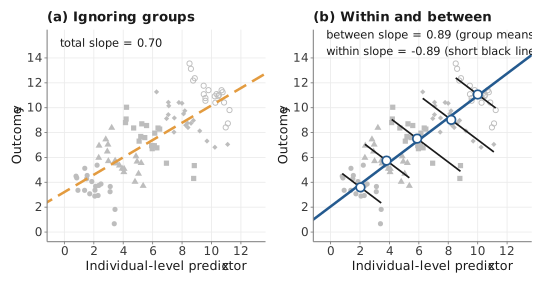
Note. Simulated data for five groups of 20 individuals; point shapes distinguish the groups. Panel (a): the dashed line is the least-squares line fitted to all 100 individuals. Panel (b): short black lines show the pooled within-group slope drawn through each group’s data; open circles are the group means and the solid line is the least-squares line through them.
1.7.2Ecological and atomistic fallacies#
Two errors of inference follow from confusing levels. The ecological fallacy is the error of drawing conclusions about individuals from relations observed among aggregates. Robinson (1950) showed that correlations computed from the averages of U.S. regions or states could differ greatly, even in sign, from the corresponding correlations among individuals. In Figure 1.6, concluding from the positive relation among group means that individuals with higher tend to have higher would be an ecological fallacy. The reverse error, the atomistic (or individualistic) fallacy, draws conclusions about groups from relations observed among individuals (Alker, 1969; Hox et al., 2018). Concluding from the negative within-group slope that groups with a higher mean on must have a lower mean on would be an atomistic fallacy.
Neither aggregation nor disaggregation solves the problem, because the problem is not the choice of a unit of analysis. Both relations exist, both can be of substantive interest, and both can be estimated. Multilevel models allow within-cluster and between-cluster relations to be estimated simultaneously and to differ, and they make it possible to ask whether they differ. How to do this, and how the answer depends on how the predictor is centered, is the subject of Chapter 7.
1.8Multilevel Theories and Propositions#
A multilevel model is a statistical representation of a substantive theory that involves more than one level. It is therefore worth stating the theory before writing any equation. Snijders & Bosker (2012, Ch. 2) give a compact way to do this, in the spirit of the macro–micro diagrams of Coleman (1990). Propositions are classified by the levels of the variables they connect; in this notation, macro-level (level-2) variables are written in capital letters and micro-level (level-1) variables in lower case. Figure 1.7 redraws the main types with UMG plates. The boundary of the inner (pupil) plate plays the role of the dotted line that separates the micro level from the macro level in Snijders and Bosker’s diagrams: variables inside the pupil plate are micro-level, and variables in the school plate but outside the pupil plate are macro-level.
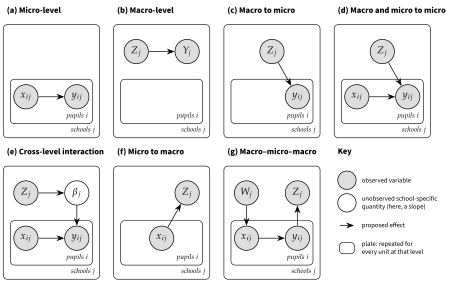
Note. Each panel shows a pupil plate nested in a school plate. Shaded circles represent observed variables; the open circle in panel (e) represents an unobserved school-specific quantity, the slope of on in school . Arrows represent proposed effects. Macro-level (school) variables are written in capitals and micro-level (pupil) variables in lower case, following Snijders & Bosker (2012).
A micro-level proposition (panel a) relates two micro-level (pupil) variables, for example a pupil’s homework time and the same pupil’s mathematics score in a study that sampled pupils within schools. The macro level plays no role in the theory, and dependence among pupils in the same school is a nuisance to be accounted for, not a subject of study. A macro-level proposition (panel b) relates two cluster-level variables, for example the average wealth of a school’s catchment area () and the school’s mean achievement (). When is not observed directly but is computed from pupil measurements, as a school mean is, the data are multilevel even though the proposition concerns only schools.
The more interesting propositions connect levels. In a macro-to-micro proposition (panel c), a cluster variable affects an individual outcome: pupils in schools with higher average SES have higher mathematics achievement. In a macro-and-micro-to-micro proposition (panel d), both a cluster variable and an individual variable affect the individual outcome: given the time a pupil spends on homework, pupils in schools with higher average SES achieve more; and given the school’s average SES, pupils who spend more time on homework achieve more. In a cross-level interaction (panel e), a cluster variable changes the relation between two individual variables. Snijders & Bosker (2012) give the example of ability grouping (): the effect of a pupil’s aptitude () on achievement () may be small in classes where pupils are grouped by ability and large in classes where they are not. In the UMG this is drawn by making the slope of on a school-specific quantity that lives in the school plate, and letting affect it. Chapter 6 estimates exactly this structure as a random slope with a cross-level interaction.
Propositions can also run upward. In a micro-to-macro (or emergent) proposition (panel f), individual characteristics affect a group-level outcome, for example pupils’ achievement affecting their teacher’s experience of stress; Kozlowski & Klein (2000) discuss such emergent processes in organizations. Finally, propositions can be chained (panel g): a teacher’s attitude toward learning () affects pupils’ attitudes (), which affect their achievement (), which in turn affects the teacher’s professional prestige (). Such chains explain through which micro-level variables two macro-level variables are associated. Models for upward and chained propositions go beyond the basic multilevel regression model; they are taken up in Chapter 29 on multilevel structural equation modeling.
1.9What Multilevel Models Offer, and What They Cost#
Multilevel models have become the standard tool for nested data because they offer several advantages over both disaggregated and aggregated analyses (Hoffman & Walters, 2022; Raudenbush & Bryk, 2002; Snijders & Bosker, 2012).
Correct inference. They represent the dependence among observations, so standard errors, confidence intervals, and significance tests are valid (under the model’s assumptions and with enough clusters), including tests of cluster-level variables.
Efficient estimation. When the model is correctly specified, they combine within-cluster and between-cluster information efficiently (Chapter 7 shows when the two kinds of information must be kept apart), and they borrow strength across clusters, so that estimates for small clusters are stabilized by information from the other clusters (Chapter 12).
Variables at every level. Explanatory variables measured at any level of the hierarchy can enter one model, and their effects can be tested at the appropriate level.
Within and between effects. Within-cluster and between-cluster relations can be estimated separately, which protects against the ecological and atomistic fallacies (Chapter 7).
Heterogeneity as a finding. Relations that vary across clusters (random slopes) and the explanation of that variation by cluster characteristics (cross-level interactions) become part of the model (Chapter 6).
Unbalanced and incomplete data. Clusters of different sizes, and in longitudinal data persons measured at different times and on different numbers of occasions, are handled without discarding data (Chapters 17 and 19).
Rich theories. Many of the propositions in Figure 1.7 can be translated directly into a model, and the model can be drawn and read as the theory it represents.
These advantages come at a cost. The tools of ordinary regression (estimation, tests, measures of fit, diagnostics) must be modified, and the modifications are not always obvious (Part III). Models with several random effects and cross-level interactions can become complex, and the number of possible models grows quickly with the number of variables and levels (Chapter 14). Estimation can fail or give implausible results, especially with few clusters or with variance components near zero (Chapter 9). And the models’ assumptions about the distribution of the random effects and about their independence from the explanatory variables must be examined rather than taken for granted (Chapters 7 and 15). Much of this book is about using multilevel models well in spite of these costs.
1.10The Range of Applications and a Map of This Book#
The applications of multilevel models extend well beyond pupils in schools. The same models are used for sample surveys with multistage designs, for school and teacher effectiveness research, for longitudinal and repeated-measures data, for discrete outcomes such as pass rates, graduation, or symptom presence, for multivariate outcomes in which several variables are measured on each individual (each response becoming a level-1 unit nested within the individual), for nonlinear growth patterns, for cross-classified designs such as participants crossed with stimuli, for measurement models in which item responses are nested within or crossed with persons (De Boeck & Wilson, 2004), for structural equation models with latent variables at several levels, for meta-analysis, in which effect sizes (or participants) are nested within studies, and for models in which the variability of an outcome, not only its mean, differs across persons or groups. Most of these applications have a chapter of their own in this book.
Table 1.6 gives the plan of the book. Part I lays the foundations: this chapter, a chapter on notation and on the three ways of writing (and the graphical way of drawing) a multilevel model, a chapter that derives the multilevel model from the analysis of variance and regression models that readers already know, and a chapter on exploring and managing multilevel data. Part II develops the core models. Part III opens the machinery of estimation and inference. Part IV turns the machinery into a workflow for building, checking, designing, and reporting analyses. Parts V to VII extend the models to longitudinal and intensive data, to generalized outcomes and non-nested structures, and to latent variables and causal questions.
| Part | Chapters | Main questions |
|---|---|---|
| I. Foundations | 1–4 | Why multilevel models? How are they written, drawn, and explored? |
| II. The core models | 5–8 | Random intercepts, random slopes, cross-level interactions, centering, three levels |
| III. Estimation and inference | 9–13 | How are the models estimated and tested? What are predicted random effects? Bayesian estimation |
| IV. Building, checking, designing, reporting | 14–18 | Model building, diagnostics, power, missing data, weights, reporting |
| V. Longitudinal and intensive data | 19–22 | Growth, covariance structures, within-person dynamics, latent curve models |
| VI. Generalized and extended models | 23–28 | Binary, ordinal, count, and survival outcomes; crossed and multiple-membership structures; multivariate and meta-analytic models; variability as an outcome |
| VII. Latent variables, causality, frontiers | 29–32 | Multilevel SEM and measurement, causal inference, alternatives and extensions |
Each later chapter follows the same pattern. It opens with a substantive question and a data set, develops the concepts, writes each new model in three ways, draws it as a Unified Model Graph, shows the data displays the model implies, works through an example with annotated R code, and closes with advice on interpretation and reporting, common pitfalls, a software crosswalk for SAS, SPSS, Stata, Mplus, HLM, and JASP, a summary, and exercises. Longer derivations are placed in Technical Detail boxes, which can be skipped on a first reading.
Key Terms#
- aggregation and disaggregation
- atomistic fallacy
- between-cluster relation
- cluster; cluster-randomized trial
- cross-classified structure
- cross-level interaction
- design effect
- ecological fallacy
- effective sample size
- empty (null) model
- intraclass correlation
- level; level-1 and level-2 units
- macro-level and micro-level propositions
- micro-to-macro (emergent) proposition
- multiple-membership structure
- multistage sampling
- plate
- Simpson’s paradox
- total relation
- unit-of-analysis problem
- within-cluster relation
Exercises#
A. Concept checks#
For each study, name the levels, the units at each level, and whether the structure is nested, cross-classified, or multiple-membership: (a) 60 therapists each treat 8 clients, and each client completes a symptom checklist weekly for 12 weeks; (b) 150 participants each judge the attractiveness of the same 40 faces; (c) employees rate their team climate, and some employees belong to two teams; (d) 2,000 adolescents from 90 neighborhoods attend 30 high schools.
In a study of pupils in schools, state the level of each variable: mathematics score, school size, pupil’s gender, proportion of girls in the school, teacher’s years of experience (one teacher per class, several classes per school), and the average homework time of the pupils in a class.
An ICC of .08 is reported for an outcome in a sample of 60 schools with 120 pupils each. A colleague concludes that “the clustering is negligible, so ordinary regression is fine.” Explain in two or three sentences why this conclusion is unsafe.
Explain the difference between the ecological fallacy and the atomistic fallacy, and give an example of each from your own field.
Classify each proposition by the types in Figure 1.7: (a) “Classrooms with a more supportive climate have lower average anxiety”; (b) “Pupils’ anxiety is lower in classrooms with a more supportive climate”; (c) “The effect of pupils’ prior achievement on anxiety is weaker in classrooms with a more supportive climate”; (d) “Pupils’ disruptive behavior increases teachers’ burnout.”
B. Analytical exercises#
Using Equation (1.1), show that for two different pupils in the same school, that for pupils in different schools, and hence that . Solution →
Derive the design effect of Equation (1.3) by following the steps in the Technical Detail box. Then show that the effective sample size lies between and , and state when each bound is reached. Solution →
A cluster-randomized trial will enroll 30 classes of 25 pupils. Pilot data suggest . Compute the design effect and the effective sample size. By how much must the number of classes be increased to obtain the same effective sample size as a trial of 30 classes with no clustering? Solution →
Using the approximation in the Technical Detail box, explain why ignoring clustering hurts tests of cluster-level predictors much more than tests of predictors that vary mainly within clusters. Solution →
C. Computational exercises#
Using
nels88_school23.csv, compute the number of pupils, the mean mathematics score, and the within-school OLS intercept and slope of mathematics on homework for each of the 23 schools. Plot the 23 regression lines in one panel, as in Figure 1.4(b). Describe how the schools differ.Reproduce Table 1.4 for two other schools of your choice, and comment on whether the pooled slope describes either school.
Fit the empty model to the NELS:88 data in R and in one other program from the crosswalk. Confirm that the estimated ICC is about .24, and compute the design effect using the average cluster size.
Using
jsp_wide.csv, compute for each school the correlation between mathematics in year 0 and year 1. Plot the correlations against the number of pupils in the school. What does the plot suggest about the reliability of school-specific estimates from small schools? Solution →
D. Simulation exercise#
Open
sim_ch01_typeI_V01.R. (a) Change the number of clusters from 40 to 10 and rerun the simulation. Does the cluster-level test still hold the .05 level? Does the OLS test behave better or worse than with 40 clusters? (b) Add a pupil-level predictor that varies only within clusters (for example, for standard normal ) and whose true effect is zero. Record how often the OLS test of this predictor rejects. Explain the result with the approximation . Save the new scripts with the suffix_V02.
E. Applied mini-project#
Choose a published empirical article in your area whose data are nested. (a) Draw the data structure as a unit diagram and with plates, placing every variable used in the analysis in the correct plate. (b) State the main research question as one or more of the proposition types in Figure 1.7. (c) Report the number of clusters and the cluster sizes, and state whether the analysis respected the design. (d) Write a short reviewer comment (about 150 words) on the unit of analysis.
Lab#
Further Reading#
- Snijders & Bosker (2012, Ch. 1–2)
-
The source of the proposition types used in this chapter, with a careful discussion of aggregation, disaggregation, and the levels of variables.
- Raudenbush & Bryk (2002, Ch. 1)
-
A history of the problems that hierarchical linear models were developed to solve, with applications from education.
- Kreft & de Leeuw (1998, Ch. 1)
-
A short and readable introduction to the unit-of-analysis problem, using the NELS:88 data analyzed in this chapter.
- Robinson (1950)
-
The classic demonstration that ecological correlations need not equal individual correlations.
- Aitkin et al. (1981)
-
The reanalysis of the teaching-styles study; the discussion that follows the paper is a good record of how the field’s thinking changed.
- Kenny & Judd (1986)
-
A clear account of how nonindependence biases tests in analysis of variance, written for psychologists.
- Kozlowski & Klein (2000)
-
A framework for multilevel theory in organizational research, including emergent (micro-to-macro) processes.
- Hoffman & Walters (2022)
-
A recent overview of multilevel modeling for psychologists, with pointers to many of the topics in later chapters.