Exploring and Managing Multilevel Data
In this chapterlevel-1 and level-2 files, merging, and reshaping; identifiers and the data audit; derived variables and their traps; exploratory displays read as model-implied displays; exploring the fixed part; exploring the random part; simulating multilevel data; a reproducible project layout.
Most errors in multilevel results are not caused by exotic estimation problems. They are caused by a merge on the wrong key, a cluster mean computed from the wrong cases, or a model fitted before anyone looked at the data. This chapter covers the work that comes before the first model: building an analysis file from pupil-level and school-level sources, computing the derived variables that multilevel models use, and exploring the data with displays that answer specific questions about the model to be fitted. The exploratory part follows the first half of the course lecture on model building, which in turn follows the logic of Raudenbush & Bryk (2002, Ch. 9) and Snijders & Bosker (2012, Ch. 10): study the mean structure first, remove it, and then study what is left.
The chapter uses the model-data duality of Chapter 2 as its organizing idea. Every element of a Unified Model Graph makes a claim about the data, and every claim has a display that can check it. The plate claims that clusters are exchangeable replicates, so it calls for one panel per cluster. A random coefficient claims that a quantity varies across clusters, so it calls for a display of that quantity cluster by cluster. Reading the displays in this way turns exploratory data analysis (Tukey, 1977) from a loose collection of plots into a systematic check of each part of the intended model. The results of that check are hypotheses about the model, not findings, and they are tested formally in Part III.
4.1Data Structures and Files#
4.1.1Level-1 and level-2 files#
Multilevel data rarely arrive as a single file. Large-scale surveys release separate files for each type of unit, and a researcher’s own study typically produces a pupil questionnaire file, a teacher or school file, and perhaps an administrative file. The TIMSS data used in the course labs illustrate the simplest case. The level-1 file has one row per pupil: 7,097 pupils in grades 3 and 4, with a school identifier (idschool), a pupil identifier (idstud), grade, gender, and mathematics and science scores. The level-2 file has one row per school: 146 schools, with the school identifier and a school characteristic from the principal questionnaire, the reported shortage of instructional materials (shortages, coded 0 = none to 3 = a lot). The identifier that appears in both files is the key that links them.
4.1.2The many-to-one merge#
Panel (a) of Figure 4.1 shows the operation that builds the analysis file. Each pupil row is matched to the one school row with the same key, and the school’s values are copied onto every pupil of that school. The result has as many rows as the pupil file, and the school variable is constant within each school. This is a many-to-one merge: many pupil rows match one school row. In R it is left_join(pupils, schools, by = "idschool"); in SAS it is a MERGE statement with a BY variable after both files have been sorted by the key; in SPSS it is MATCH FILES with a /TABLE subcommand, and in Stata merge m:1.
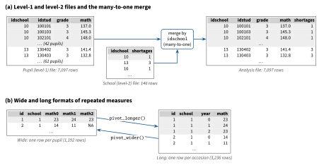
Note. Panel (a): the first rows of the TIMSS pupil file and school file used in the course labs, and of the merged analysis file; rows with a gray fill belong to school 10. Panel (b): the first rows of the Junior School Project mathematics scores in wide format (one row per pupil, one column per year) and long format (one row per pupil and year); NA = missing.
Three checks belong to every merge. First, the key must be unique in the level-2 file; if a school appears twice, every pupil of that school is duplicated (a many-to-many merge). Second, the number of rows after the merge must equal the number of pupil rows. Third, pupils without a matching school, and schools without pupils, must be counted and explained rather than silently dropped. In R, the argument relationship = "many-to-one" of left_join() (dplyr 1.1.1 or later) stops with an error if a pupil’s key matches more than one school row, which enforces the first check and therefore the second; the script prepare_timss_V01.R uses it. Unmatched units must still be counted separately, for example with anti_join().
4.1.3Long and wide formats#
Repeated measures can be stored in two ways (panel b of Figure 4.1). In wide format each person has one row and each occasion has its own column (math0, math1, math2 for the three years of the Junior School Project). In long format each occasion has its own row, with a variable that records the occasion (year). Most multilevel software requires the long format, in which occasions are the level-1 units, exactly as pupils are in the TIMSS file. The long format is also the tidy arrangement of Wickham (2014): each variable is a column, each observation is a row, and each type of unit has its own table. Two features of the long format matter later. A missing occasion is simply an absent row (pupil 2 has no row for year 2), so persons with incomplete data stay in the analysis (Chapters 17 and 19). And a time-varying predictor, such as the age at each occasion, becomes an ordinary level-1 variable. In R, tidyr::pivot_longer() and pivot_wider() convert between the formats (Wickham et al., 2023, Ch. 5).
4.1.4Identifiers#
Identifiers deserve more care than any other variable, because an error in an identifier changes the structure of the data without changing a single score. Three rules prevent most problems. First, every unit needs an identifier that is unique across the whole data set, not only within its cluster. In the NELS:88 file the student number restarts in each school (the 519 pupils share 100 different student numbers), so a unique pupil identifier must combine the school and student numbers; in the Junior School Project the class number runs from 1 to 4 within each school. Second, identifiers that encode structure should be decoded and checked. The TIMSS pupil identifier has the form school, class, pupil: pupil 102101 is pupil 01 in class 21 of school 10. Dropping its last two digits (integer division by 100) therefore gives a class identifier that is unique across schools, and the data turn out to have a third level, 414 classes, that the lab file does not mention. Third, level-2 variables must be constant within clusters; a school variable that takes two values within one school signals a coding or merge error. The script prepare_timss_V01.R checks all three.
4.1.5The data audit#
Before any model is fitted, a short data audit describes the structure: the number of level-1 and level-2 units, the distribution of cluster sizes, the number of singletons (clusters with a single level-1 unit), and the intraclass correlation of the outcome. Table 4.1 gives the audit for the data sets of this chapter. It is worth a careful look. The TIMSS schools are large (median 48.5 pupils), but the classes within them are small, and one class has a single pupil. The Junior School Project has about 2.7 occasions per pupil and 35 pupils with only one occasion. The sleep deprivation study is perfectly balanced, with ten days for each of 18 subjects. The intraclass correlations range from .20 to .63. Each of these facts affects later decisions: small clusters limit what can be learned about within-cluster slopes, singletons contribute nothing to within-cluster estimates, and a small number of clusters (18 subjects, 23 schools) limits what can be learned about variance components (Chapter 16).
| Unit | Cluster size | ||||||||
|---|---|---|---|---|---|---|---|---|---|
| Data set | Level 1 | Level 2 | Min | Median | Max | ICC | |||
| NELS:88 | Pupil | School | 519 | 23 | 5 | 21 | 67 | 0 | .24 |
| TIMSS | Pupil | School | 7,097 | 146 | 7 | 48.5 | 83 | 0 | .20 |
| TIMSS | Pupil | Class | 7,097 | 414 | 1 | 17 | 30 | 1 | .32 |
| JSP | Occasion | Pupil | 3,236 | 1,192 | 1 | 3 | 3 | 35 | .63 |
| Sleep study | Day | Subject | 180 | 18 | 10 | 10 | 10 | 0 | .39 |
Note. NELS:88 = National Education Longitudinal Study of 1988, subsample of 23 schools; TIMSS = U.S. pupils in grades 3 and 4 in the course lab file; JSP = Junior School Project, mathematics in years 0 to 2 (occasions nested in pupils, schools ignored here); Sleep study = sleep deprivation study, reaction time on days 0 to 9. = number of level-1 units; = number of level-2 units; = cluster size; = number of singleton clusters. ICC = intraclass correlation of the outcome from the empty model estimated by restricted maximum likelihood. TIMSS classes are decoded from the pupil identifiers.
4.2Derived Variables#
Multilevel models use a small set of variables computed from the raw data (Table 4.2). The most important are the cluster mean of a level-1 variable, , which can serve as a level-2 predictor; the group-mean-centered variable , which contains only within-cluster variation; and the grand-mean-centered variable , which only moves the origin. The TIMSS lab computes all three for mathematics: grpMmath (the school mean), grpCmath (mathematics minus the school mean), and OCmath (mathematics minus the overall mean of 151.09). Chapter 7 discusses what these variables mean in a model and how to choose among them (Enders & Tofighi, 2007; Kreft et al., 1995). Here the concern is to compute them correctly.
| Derived variable | Definition | R (after group_by(cluster))
| Use and caution |
|---|---|---|---|
| Cluster size | n_j = n()
| Report its distribution; flag singletons () and very small clusters. | |
| Cluster mean | x_mean = mean(x, na.rm = TRUE)
| Level-2 (compositional) predictor. Decide and report which cases enter the mean. | |
| Group-mean-centered variable | x_cwc = x - mean(x, na.rm = TRUE)
| Pure within-cluster predictor; its cluster means are zero. Equals 0 for every singleton. | |
| Grand-mean-centered variable | x_cgm = x - mean(x) (ungrouped)
| Moves the origin only; the model fit is unchanged. | |
| Centered cluster mean | x_mean - mean(x) (ungrouped)
| Level-2 predictor with a meaningful zero. | |
| Cluster proportion | = mean of a 0/1 indicator | p_white = mean(white)
| Composition of the cluster (e.g., proportion of girls). |
| Cluster standard deviation | x_sd = sd(x)
| Heterogeneity of composition; undefined when . | |
| Within-cluster relative standing | or rank | x_rank = rank(x) / n()
| Position of a unit relative to its own cluster (“big fish, little pond”). |
Note. = value of level-1 unit in cluster ; = cluster mean; = grand mean over all level-1 units; = within-cluster standard deviation. The R expressions assume the tidyverse (dplyr).
The three variables are linked by an identity that is worth remembering, because it shows that nothing is lost by centering:
A model that includes both the group-mean-centered variable and the cluster mean therefore uses all the information in , but lets its within-cluster and between-cluster parts have different coefficients. This is the model-based version of the within and between regressions of Chapter 3.
4.2.1Computational traps#
Four traps recur in practice. The first is missing data in cluster means. If some pupils lack a mathematics score, the school mean can be computed from all pupils with a score or only from the pupils who enter the final analysis (those with complete data on every model variable). The two means differ, and the choice changes the between-school coefficient. Neither is always right, but the choice must be deliberate and reported; the usual recommendation is to use all available level-1 information for a cluster characteristic that is meant to describe the cluster. The second trap is recomputing after subsetting. Means computed before cases are excluded (for example, before restricting the sample to grade 4) describe a different population than the analysis sample, and centered variables no longer have cluster means of zero in the subset. Compute derived variables at the point in the pipeline where the analysis sample is fixed, and check that the group-mean-centered variable averages zero in every cluster. The third trap is singletons and tiny clusters. A group-mean-centered variable is exactly zero for a singleton, and the cluster mean of a cluster of two is a poor measure of the cluster. Such clusters are legitimate members of the data (they contribute to the between-cluster part of the model), but the audit should count them. The fourth trap is sampling error in cluster means. The observed mean of 20 pupils is an estimate of the school’s true mean, not the true mean itself, and using it as a predictor biases the between-cluster coefficient toward the within-cluster coefficient (and hence the contextual effect toward zero); the bias is largest when clusters are small and the ICC of the predictor is low. Chapter 7 presents the latent-mean solution.
4.3Displays as Model-Implied Displays#
Chapter 2 introduced the model-data duality: every element of a model implies a display of the data. Table 4.3 turns this idea into a checklist for the random intercept and slope model, the model that most two-level analyses in this book start from. The left column lists the elements of its Unified Model Graph (Figure 2.4(c)), the middle columns state what each element claims about the data and which display checks the claim, and the right column points to the examples in this chapter.
| UMG element | Claim about the data | Display and what to look for | Example |
|---|---|---|---|
| Pupil plate nested in school plate | Pupils are exchangeable within schools, schools within the population | Data audit; trellis with one panel per cluster: does the same kind of relation appear in every panel? | Table 4.1, Figure 4.3 |
| Edge with diamond | The mean of changes linearly with , in the same way in all sub-populations | Pooled scatter with smoothers; means at each level of by sub-population: straight, curved, parallel, crossing? | Figures 4.2, 4.4 |
| Open circle with loop | Cluster intercepts vary around | Caterpillar of cluster intercepts: is the spread larger than the intervals imply? | Figure 4.5a |
| Open circle with loop | Cluster slopes vary around | Spaghetti and trellis lines, caterpillar of slopes: do the lines fan out more than sampling error allows? | Figures 4.3, 4.5b, 4.6 |
| Covariance edge | Intercepts and slopes are related | Scatter of cluster intercepts against slopes: is there a trend? | Figure 2.6c |
| Residual stub with random slope | Marginal variance is quadratic in (the variance function) | Squared OLS residuals against : flat band or U shape? | Figure 4.7 |
| All random terms together (marginal ) | A specific pattern of within-cluster correlation | Correlation map of residuals: constant, decaying with lag, rising over time? | Figure 4.8 |
Note. UMG = Unified Model Graph (Chapter 2). = fixed effects; = cluster-specific intercept and slope; = their variances and covariance; = level-1 residual variance; = marginal covariance matrix of the outcomes of cluster . OLS = ordinary least squares.
The table suggests an order of work that mirrors the order of the model: first the fixed part (the diamonds and the edges from predictors to the outcome), then the random part (the open circles, their loops, and the covariance edge), and finally the pattern of dependence that the random part implies. The order matters because the displays of the random part use residuals, and residuals are meaningful only after a reasonable fixed part has been removed.
4.4Exploring the Fixed Part#
4.4.1Why the fixed part comes first#
The random part of a multilevel model describes the variation that the fixed part leaves unexplained. A random slope, for instance, may be needed only because a curve was fitted as a straight line, or because a cross-level interaction was left out. For this reason the course lecture on model building starts with a deliberately generous preliminary fixed part: all the level-1 and level-2 predictors, curves, and interactions that theory or the displays suggest. Its purpose is to remove the systematic variation from the data so that the remaining variation can be studied. The preliminary fixed part can be estimated by ordinary least squares, ignoring the clustering, because OLS estimates of the fixed effects are unbiased and consistent under a multilevel model as long as the fixed part is correctly specified and the predictors are unrelated to the random effects and the level-1 residuals; only their standard errors are wrong (Chapter 1). The residuals of that OLS fit are then the raw material for exploring the random part (Section 4.5).
4.4.2Pooled displays#
The first displays ignore the clusters. Panel (a) of Figure 4.2 plots mathematics against weekly homework time for all 519 NELS:88 pupils, with the mean at each homework level, the OLS line, and a natural cubic spline with three degrees of freedom as a flexible smoother. Mean mathematics is flat, around 48 to 50 points, for pupils reporting at most one hour of homework (categories 0 to 2) and then rises steeply to about 61 points from three hours upward (categories 4 to 7), where it levels off. The straight line (slope 3.13 points per homework category) misses this shape: it lies about 3 points below the means in categories 0 and 4, slightly above them in categories 1 and 2, and 3 to 6 points above the means of the few pupils in categories 6 and 7. Because the categories are not equally spaced in hours (category 5 alone spans four to six hours), a slope per category is not a slope per hour. The spline follows the means closely. A formal comparison of the two OLS fits favors the spline, , but its value (.008) ignores the clustering and is therefore too small (Chapter 1); at this stage the comparison is descriptive. Note also how few pupils report seven hours or more (categories 6 and 7, with 6 and 3 pupils): the shape at the upper end rests on very little data.
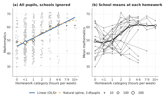
Note. Panel (a): gray points are pupils (jittered horizontally); diamonds are the mean at each homework level, with area proportional to the number of pupils; the solid line is the OLS regression line and the dashed curve a natural cubic spline with 3 degrees of freedom. Panel (b): each thin line joins the mean mathematics scores of one school at the homework levels observed in that school; the thick line and diamonds are the overall means from panel (a). Homework is recorded in ordered categories; tick labels give the hours per week that each category represents.
Panel (b) of Figure 4.2 takes a first step toward the clusters by joining, for each school, the mean score at each homework level. The overall means (thick line) hide a great deal of variety. In some schools the means rise with homework, in others they fall, and many schools are too small to show a clear pattern at all. This display is useful mainly as a warning that the pooled curve in panel (a) is an average of different school curves; the trellis display shows them properly.
4.4.3The trellis display#
A trellis display (also called small multiples or a lattice display) shows one panel per cluster, with the same axes in every panel (Becker et al., 1996); it builds on the conditioning plots of Cleveland (1993). It is the display implied by the plate: if the clusters are exchangeable replicates of one model, every panel should show the same kind of relation, with cluster-specific details. Figure 4.3 shows all 23 NELS:88 schools, ordered by the slope of the within-school OLS regression of mathematics on homework. Ordering is essential. In alphabetical or identifier order, the panels would look like a random collection; ordered by slope, they reveal a systematic progression from eight schools in which mathematics falls with homework (slopes from to points per homework category) to fifteen in which it rises (from to ).
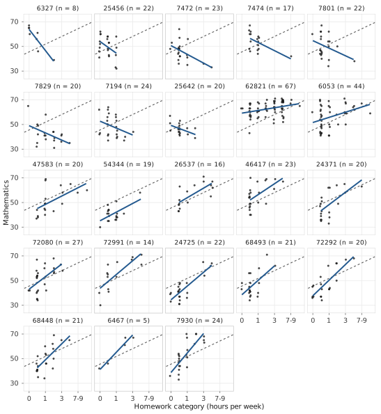
Note. One panel per school, labeled with the school identifier and number of pupils, ordered by the within-school OLS slope from smallest (top left) to largest (bottom right). Points are pupils (jittered horizontally); the solid segment is the within-school OLS line drawn over the range of homework observed in that school; the dashed line is the pooled OLS line for all 519 pupils.
Three features of Figure 4.3 guide the model. First, within most schools the relation looks roughly linear; there is little sign that the curve in Figure 4.2(a) is present within schools. The curve may therefore be a between-school phenomenon: schools whose pupils do more homework have higher means (a question for Chapter 7). Second, the slopes differ so much, and in sign, that a model with a common slope (a random intercept model) would misrepresent most schools. Third, the panels differ in size and in the range of homework they cover: school 6467 has 5 pupils, school 62821 has 67, and three schools have no pupil who reports more than two hours of homework (none above category 3). How much each panel can tell about its school’s slope depends on these features, a point taken up in Section 4.5.
4.4.4Averaging over sub-populations#
The trellis display shows clusters. A means-by-covariate display shows sub-populations defined by other predictors instead: it plots the mean outcome at each level of one predictor, separately for the groups of a second predictor. Parallel profiles suggest additive effects; profiles that diverge or cross suggest an interaction. Figure 4.4 applies it to three predictors that the course lecture examines: pupil race (White or not), gender, and school sector.
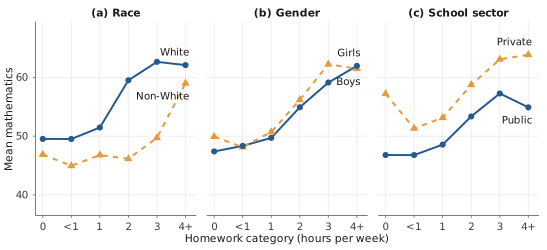
Note. Each point is the mean mathematics score of the pupils in one group at one homework level; homework categories 5, 6, and 7 (four hours or more per week) are combined and labeled 4+, and the other tick labels give the hours per week of each category. Solid lines with circles and dashed lines with triangles distinguish the two groups of each panel; group names are printed next to the last point of each profile.
The three panels tell three different stories. In panel (a), White pupils score higher than non-White pupils at every homework level, and the gap, about 3 to 5 points among pupils reporting at most one hour of homework (categories 0 to 2), exceeds 12 points at two and three hours (categories 3 and 4) and narrows again to about 3 points at four hours or more. This suggests an interaction of homework and race, but the evidence is thin: only 26 of the 129 non-White pupils report two hours or more (categories 3 to 7), and the non-White mean for four hours or more (categories 5 to 7 combined) rests on 5 pupils. In panel (b), the profiles of girls and boys nearly coincide, which suggests neither a gender effect nor a gender by homework interaction. In panel (c), pupils in private schools score higher than pupils in public schools at every homework level, by 4.5 to 6 points in categories 1 to 4 and by about 9 to 10 points at the two ends, where one of the two means rests on few pupils (9 private-school pupils in category 0, 11 public-school pupils at four hours or more). Over the well-populated middle of the range the profiles are roughly parallel, which suggests an additive sector effect. Because private-school pupils also report more homework (mean homework category 2.5 versus 1.6), part of the pooled homework slope in Figure 4.2 may reflect sector rather than homework, another reason to separate within-school and between-school relations.
Sector is a school-level variable, so panel (c) compares two groups of schools, not two groups of pupils; the information about the sector difference is governed by the number of schools (8 private, 15 public) much more than by the number of pupils. Displays of level-2 predictors should therefore be read with the school as the unit, for example by plotting school means or school slopes against the school variable, as in the second stage of the two-stage analysis in Chapter 3.
4.4.5Curves: polynomials and splines#
When a display suggests a curve, two tools are available for exploration. A polynomial adds (and perhaps ) to the model; it is easy to interpret near the center of the data but can behave badly at the edges. A regression spline joins low-order polynomial pieces at chosen points (knots); natural cubic splines, as in Figure 4.2(a), are constrained to be linear beyond the outer knots and are therefore more stable at the edges. Both are fixed-effects terms and can be carried into the multilevel model. In exploration, their main use is to answer a yes-or-no question: is there curvature that a straight line would miss? If the answer is yes, the final model can use whichever form is most interpretable, and Chapter 14 discusses how to choose.
4.5Exploring the Random Part#
4.5.1Within-cluster regressions and their precision#
The random coefficients and of the model have natural estimates in the data: the intercept and slope of an OLS regression within each cluster, the stage-one estimates of the two-stage approach in Chapter 3. The caterpillar display plots these estimates, sorted by size, with their confidence intervals (Figure 4.5). Homework is centered at its grand mean of 1.97, almost exactly category 2 (“one hour”), so each intercept estimates the expected score of a pupil in that school with homework at the grand mean.
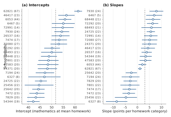
Note. Each row is one school, labeled with its identifier and, in parentheses, its number of pupils; rows are sorted by the estimate within each panel. Open circles are OLS estimates from the regression of mathematics on homework (homework category centered at its grand mean of 1.97) within the school; horizontal segments are 95% confidence intervals based on the distribution. The dashed vertical line is the pooled OLS estimate.
The caterpillar answers the question that the trellis cannot: is the spread of the estimates larger than sampling error alone would produce? If all schools had the same true slope, the estimated slopes would still differ, but their spread would be of the same size as their standard errors, and most intervals would overlap the pooled value. In panel (b) the opposite is true. The intervals of 14 of the 23 schools exclude the pooled slope (and 21 exclude zero), and the intervals of the negative-slope and positive-slope schools barely overlap. A rough numerical version of the same comparison uses the logic of Chapter 3: the variance of the 23 OLS slopes is 21.8, while the average squared standard error is only 1.9, so about of the variance appears to reflect true differences between schools. This moment-type estimate is close to the REML estimate of the random slope model in Chapter 2 (Table 2.2). The same comparison for the intercepts gives . Both comparisons suggest that the random intercept and slope model is a reasonable starting point for these data.
The caterpillar is also a reminder that precision differs between clusters. The interval of a school depends on its size, its residual variance, and the spread of homework within it. School 62821, with 67 pupils and a wide range of homework, has the narrowest slope interval; the multilevel model will give it the most weight in estimating the average slope. Here, however, is much larger than every school’s sampling variance, so the weights differ by at most about a quarter and the multilevel estimate stays close to the unweighted two-stage mean; the weighting matters most when the true slopes vary little.
4.5.2Spaghetti displays for longitudinal data#
For repeated measures, the display implied by a random slope is the spaghetti display: one line per person across time. Figure 4.6 shows the reaction times of the 18 subjects of the sleep deprivation study (Belenky et al., 2003), a data set distributed with lme4 (Bates et al., 2015). The lme4 documentation notes that days 0 and 1 were adaptation and training days, day 2 was the baseline, and sleep deprivation started after day 2; like most textbook analyses, the displays here use all ten days. Panel (a) shows the observed trajectories, panel (b) the OLS line of each subject, and both show the pooled OLS line (reaction time increases by 10.5 ms per day on average).
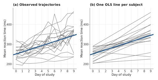
Note. Panel (a): each gray line joins the daily mean reaction times of one of the 18 subjects. Panel (b): each gray line is the OLS regression line of one subject. In both panels the thick line is the pooled OLS line for all 180 observations.
The two panels serve different purposes. The observed trajectories in panel (a) show the raw material, including the day-to-day noise and a few irregular subjects; they are the display to inspect for data errors and for nonlinear change. The fitted lines in panel (b) remove the noise and show the two features a random slope model describes: subjects start at different levels (the OLS intercepts have a standard deviation of 29 ms), and their reaction times change at different rates (the slopes range from to ms per day). The same moment comparison as for the schools applies: the variance of the 18 OLS slopes is 43.0, whereas the average squared standard error is only 7.9.
4.5.3The variance function#
A random slope has a second, less obvious consequence. Chapter 2 showed that the marginal variance of the outcome is then a quadratic function of the predictor,
whereas under a random intercept model it is the constant . Because the OLS residuals of the preliminary fixed part estimate , the expected value of their squares is approximately given by Equation (4.2). Plotting the squared residuals against therefore checks the random slope from a different angle than the trellis and the caterpillar. Table 4.4 collects what the residuals and their summaries should look like under each model; it is adapted from the course lecture.
| Statistic | Random intercept | Random intercept and slope | Display |
|---|---|---|---|
| against in each cluster: flat and parallel, or tilted and fanning | |||
| against : constant spread, or spread that changes with | |||
| against with a smoother: flat, or quadratic | |||
| (given ) | Within-cluster residual variances: similar in all clusters | ||
| Depends on and | Correlation map (longitudinal data) |
Note. = residual of level-1 unit in cluster ; and = cluster means of the residuals and of the predictor. The expressions ignore the estimation error in , which is small when the number of clusters is large.
Figure 4.7 shows the display three times. Panels (a) and (b) use data simulated from the models of the course lecture, with 100 clusters of 10 units, so that the truth is known: in (a) only the intercepts vary, in (b) the slopes vary too (, , , ). The squared residuals are strongly right-skewed, so the eye must rely on the smoother rather than on the cloud of points. In (a) the smoother is flat and follows the true variance of 5; in (b) it follows the U shape of the true variance function , with the expected noise at the edges, where there are few observations.
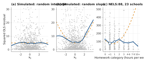
Note. Gray points are squared residuals from the OLS regression of the outcome on the predictor, ignoring clusters (NELS:88 points jittered horizontally). Panels (a) and (b): data simulated with 100 clusters of 10 units; the solid curve is a loess smoother and the dashed curve the true variance function. Panel (c): the solid line joins the mean squared residual at each homework level (circle area proportional to the number of pupils); the dashed curve is the variance function implied by the REML estimates of the random intercept and slope model in Chapter 2. The vertical axes are truncated.
Panel (c) applies the display to the NELS:88 schools, with the mean squared residual at each homework level. The result is a surprise: there is no U shape. Apart from the three pupils in category 7 (10 hours or more), the mean squared residual varies between about 80 and 127 without a trend, whereas the random slope model fitted in Chapter 2 implies a variance that rises from about 76 in category 2 (one hour) to 283 in category 5 (four to six hours; dashed curve). The trellis and the caterpillar suggested strongly varying slopes, but the variance function does not reflect them. The discrepancy is instructive, and it has at least two explanations. First, the variance function describes the spread of the school regression lines at each value of homework, extrapolated over the whole range for every school, while the display can only see pupils who actually report that much homework. Of the 47 pupils reporting four hours or more (categories 5 to 7), 22 attend one school (62821), and the eight schools with negative slopes contribute only four pupils to that range. Where the model extrapolates the steep negative lines, the data have almost no pupils. Second, a linear random slope may be the wrong description: the within-school relation may flatten at high homework levels, as the pooled means suggest. A third, more mundane factor blurs the display: the residuals come from a linear preliminary fixed part, whereas the pooled means are curved, so the misfit adds to the mean squared residual at some homework levels (one more reason for a generous preliminary fixed part). The squared misfit is at most about 12 (at category 0) and almost zero at category 5, however, so it cannot explain the missing U. The display does not decide between these explanations, but it flags the random slope specification as something to examine carefully in Chapters 6 and 14, for example by modeling the between-school part of homework separately.
4.5.4Correlation maps#
The random part of the model also implies a specific pattern of correlation among the outcomes of the same cluster, the marginal covariance matrix of Chapter 2. In cross-sectional data the units within a cluster have no natural order, and under a random intercept model the pattern reduces to a single number, the ICC. In longitudinal data the occasions are ordered, and the pattern can be displayed directly. Reshape the OLS residuals to wide format (one column per occasion) and compute their correlations across persons: this is the correlation map in panel (a) of Figure 4.8. Panels (b) and (c) show the correlations implied by two fitted models: a random intercept model, which implies the same correlation (.59) for every pair of days (compound symmetry), and a random intercept and slope model, which implies correlations that decline with the distance between days and increase over the course of the study, as the lines of Figure 4.6(b) fan out.
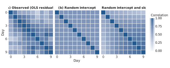
Note. Each cell shows the correlation between two days, darker for larger values. Panel (a): correlations across the 18 subjects of the residuals from the pooled OLS regression of reaction time on day. Panels (b) and (c): correlations implied by the REML estimates of a random intercept model and of a random intercept and slope model, respectively.
The observed map resembles panel (c) more than panel (b): correlations between distant days (day 0 with day 9: .52) are lower than those between adjacent days (on average .80), and the correlations among days 5 to 9 (mean .74) are somewhat higher than those among days 0 to 4 (mean .68), although much less so than the random slope model implies (.78 versus .51). The resemblance is not uniform, however: the early days correlate more strongly than the random slope model implies, and for the most distant pair the observed value lies closer to the random intercept value (.59) than to the random slope value (.30). The random slope model reproduces the general pattern but not its strength near the diagonal, where the observed correlations of adjacent days (.80) exceed the implied ones (.67). This suggests that residuals on neighboring days are correlated beyond what random intercepts and slopes can produce, a pattern that Chapter 20 models with autocorrelated level-1 errors. With only 18 subjects each observed correlation has a standard error of roughly .10 to .20, so the map should be read for its overall pattern, not for individual cells.
4.6Simulating Multilevel Data#
Simulation is the fastest way to learn what multilevel data look like. When data are generated from a known model, every display and every estimate can be compared with the truth: panels (a) and (b) of Figure 4.7 could be read with confidence only because the true variance functions were known. Simulation serves three further purposes in this book. It checks an analysis (does the software recover parameters that were put into the data?), it evaluates methods (how biased is an estimator, how often does an interval cover the true value?), and it helps design studies (how many clusters are needed for a given power? Chapter 16).
4.6.1Plates are loops#
Writing a simulation is easiest when it starts from the model graph. Figure 4.9 shows the random intercept and slope model twice, as a Unified Model Graph and as a program. The correspondence is direct. The diamonds, which represent fixed parameters, are set once, before any loop. Each plate becomes a loop: the school plate is the outer loop over , and the pupil plate, nested inside it, is the inner loop over . Each node is generated inside the loop of the innermost plate that contains it. The open circles and sit in the school plate, so they are drawn once per school, jointly from a bivariate normal distribution with covariance matrix (the loops , and the edge ). The shaded circles and sit in the pupil plate, so they are drawn once per pupil, and is computed from its parents in the graph plus a residual with variance . The same reading works for any model in this book: three-level models add a third loop, crossed factors add loops that are not nested, and a binary outcome replaces the last line with a draw from a Bernoulli distribution.
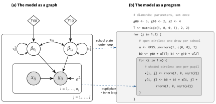
Note. Panel (a): Unified Model Graph of the random intercept and slope model (as in Figure 2.4(c)). Panel (b): R code that generates data from the model with explicit loops; the light gray box is the loop over schools and the dark gray box the loop over pupils. Dashed arrows link each plate to its loop. Comments name the graph elements generated on each line.
In practice the loops are replaced by vectorized code, which is shorter and much faster. The generator gen_mlm() of the book’s simulation template draws the random effects of all clusters in one call, draws all and at once, and uses the cluster index of each row to pick up its cluster’s random effects:
gen_mlm <- function(J, n, g00, g10, tau0sq, tau1sq, tau01, sigma2, var_x) {
  T <- matrix(c(tau0sq, tau01, tau01, tau1sq), 2, 2)
  u <- MASS::mvrnorm(J, mu = c(0, 0), Sigma = T)        # school plate
  d <- data.frame(cluster = rep(seq_len(J), each = n),   # pupil plate
                  x = rnorm(J * n, 0, sqrt(var_x)))
  d$y <- g00 + u[d$cluster, 1] + (g10 + u[d$cluster, 2]) * d$x +
         rnorm(J * n, 0, sqrt(sigma2))
  d
}4.6.2The simulation template#
A simulation study is a small experiment, and it should be planned and reported like one. Morris et al. (2019) summarize the plan in five parts: the aims, the data-generating mechanisms (the population models and the conditions varied), the estimands (the quantities to be estimated), the methods being compared, and the performance measures (bias, empirical and model-based standard errors, coverage, and their Monte Carlo standard errors). The book’s template, sim_ch04_template_V01.R, implements this plan in six labeled blocks, and every simulation script in later chapters uses the same blocks: packages and setup; simulation conditions (one row per condition, each with its own seed); the data-generation function; the analysis function; the main loop, which saves each finished condition to a checkpoint file, skips conditions already saved when restarted, and prints its progress; and the result export, which saves every replication in .rds and .csv format together with the conditions, the seeds, and the R session information. A separate analysis script (analysis_ch04_template_V01.R) reads the saved results and produces the summary table, so the expensive simulation never has to be rerun to change a table. Packages such as SimDesign (Chalmers & Adkins, 2020) provide the same structure in ready-made form.
The template’s demonstration study asks a question raised in Chapter 3: what happens to inference about the average slope when slopes vary but the model has only a random intercept? Data are generated from the random intercept and slope model of Figure 4.9 with the parameter values of the course lecture (, , , , , ), with 20 or 100 clusters of 5 or 20 units each and 500 replications per condition. Each data set is analyzed with a random intercept model and with the correct random intercept and slope model (REML, lme4). The whole study runs in about two minutes.
| Model | Bias | Empirical | Model | Coverage (%) | Singular (%) | Mean | ||
|---|---|---|---|---|---|---|---|---|
| 20 | 5 | RI | 0.013 | 0.306 | 0.179 | 75.8 (1.9) | ||
| RIS | 0.012 | 0.278 | 0.274 | 94.2 (1.0) | 8.8 | 0.99 | ||
| 20 | 20 | RI | 0.010 | 0.240 | 0.087 | 52.6 (2.2) | ||
| RIS | 0.005 | 0.234 | 0.232 | 91.8 (1.2) | 0.0 | 0.99 | ||
| 100 | 5 | RI | 0.008 | 0.136 | 0.081 | 73.2 (2.0) | ||
| RIS | 0.003 | 0.126 | 0.126 | 93.4 (1.1) | 0.0 | 1.00 | ||
| 100 | 20 | RI | 0.002 | 0.112 | 0.039 | 49.4 (2.2) | ||
| RIS | 0.002 | 0.108 | 0.105 | 94.4 (1.0) | 0.0 | 1.00 |
Note. = number of clusters; = cluster size; RI = random intercept model; RIS = random intercept and slope model (the true model). Data generated from a random intercept and slope model with and ; 500 replications per condition. Bias = mean estimate minus 2; empirical = standard deviation of the estimates; model = mean of the estimated standard errors; coverage = percentage of nominal 95% Wald intervals that contain 2, with its Monte Carlo standard error in parentheses; singular = percentage of fits with a variance or correlation estimate on the boundary of the parameter space; mean = mean REML estimate of the slope variance.
Table 4.5 shows the results. Both models estimate the average slope with negligible bias: the bias never exceeds 0.013 in absolute value, against a true value of 2. The main difference lies in the standard errors. The random intercept model reports standard errors that are far too small, 0.04 when the actual variability of its estimates is 0.11 in the largest condition, so its nominal 95% intervals cover the true value only 49% to 76% of the time. The random intercept and slope model reports standard errors that match the empirical ones, and its coverage is close to 95%, slightly below with 20 clusters of 20 (91.8%), a small-sample problem that Chapter 10 addresses. With 20 clusters of 5 units, 8.8% of the correct model’s fits are singular: the data are too sparse to estimate the covariance matrix of the random effects, even though it is not singular in the population (Chapters 9 and 11). The REML estimates of average close to the true value of 1 in every condition.
4.7A Reproducible Project Layout#
A multilevel analysis produces many files: raw data, derived data, scripts for data management, exploration, models, and figures, and the outputs they create. A fixed folder layout, used for every project, makes the work reproducible by others and by its author a year later. The layout used for this book, and recommended for the exercises and labs, is:
project/
  README.md          purpose, data sources, build order, software versions
  Data/raw/          original files, never edited (read-only)
  Data/              analysis files built by scripts (.rds and .csv)
  Scripts/           one script per task, numbered in run order
  Results/           model objects, simulation output, checkpoints
  Figures/  Tables/  outputs, always regenerated from scripts
  Notes/             decisions, open questions, the EDA memo
A few habits make the layout work (Wilson et al., 2017). Raw data are never edited; every change happens in a script that reads the raw file and writes a new one, so the path from the original data to every number in a report can be retraced. Every figure and table is produced by a script, and the output file is never edited by hand. Scripts refer to files through one root folder variable (in this book MLM_BOOK_ROOT), so the project runs on another computer after one line is changed. Scripts that draw random numbers set a seed. Substantive revisions of a script are saved under a new version suffix (_V01, _V02) instead of overwriting the earlier version, so the script that produced a published result remains available. Finally, the versions of R and of the packages used are recorded with the results, for example with sessionInfo() as in the simulation template, or with the renv package for a complete record of the package library.
Key Terms#
- caterpillar display
- cluster mean
- correlation map
- data audit
- group-mean and grand-mean centering
- key (identifier)
- level-1 and level-2 files
- long and wide format
- many-to-one merge
- means-by-covariate display
- preliminary fixed part
- regression spline
- singleton cluster
- spaghetti display
- trellis display
- variance function
- simulation template
- plates as loops
Exercises#
A. Concept checks#
For each of the following model elements, name the display that checks it and describe what the display would show if the element were not needed: (a) a random intercept; (b) a random slope; (c) the covariance ; (d) an interaction between a pupil-level and a school-level predictor.
A researcher merges a pupil file with 4,800 rows and a school file with 120 rows and obtains an analysis file with 5,230 rows. List the possible causes and the checks that would find the problem.
Explain why a group-mean-centered predictor is exactly zero for every singleton cluster, and what this implies for the information singletons contribute to a within-cluster slope.
In panel (c) of Figure 4.4, the precision of the sector comparison is governed by the 23 schools rather than the 519 pupils. Explain why, and name a display that uses the school as the unit.
B. Analytical exercises#
Show that adding the group-mean-centered variable to the grand-mean-centered cluster mean reproduces the grand-mean-centered raw variable, and that the group-mean-centered variable is uncorrelated with every cluster-level variable in the sample. Solution →
Using the Technical Detail box “OLS under a multilevel model” in Section 4.4, show that the OLS estimator of is unbiased under the random intercept and slope model and derive its covariance matrix. Under what condition is the usual OLS covariance matrix correct? Solution →
Derive under the random intercept and slope model, treating as known, and show that the minimum of the variance function lies at . Where does the minimum lie for the NELS:88 estimates of Chapter 2? Solution →
For clusters with equal size and equal spread of , show that the expected variance of the within-cluster OLS slopes is , where is the common sampling variance of a slope. Use the result to justify the moment comparison in Section 4.5. Solution →
C. Computational exercises#
Build the TIMSS analysis file from
timss_pupils.csvandtimss_schools.csvwith a checked many-to-one merge. Computen_j,grpMmath,grpCmath, andOCmath, and verify thatgrpCmathaverages zero in every school. Reproduce the TIMSS rows of Table 4.1. Solution →With science as the outcome and mathematics as the predictor, produce the TIMSS versions of Figure 4.3 (for a random sample of 25 schools), Figure 4.5, and Figure 4.7(c). Which model do the displays suggest?
Convert the Junior School Project data from long to wide format and back, and check that no information is lost. Draw a spaghetti display for the pupils of one school.
Draw the correlation map of Figure 4.8(a) using only days 2 to 9 of the sleep deprivation study. Does the pattern change?
D. Simulation exercises#
Using
gen_mlm(), simulate one data set with (all other values as in Figure 4.7b) and draw the variance function display. Where is its minimum, and does it agree with exercise B3? Solution →Save a copy of
sim_ch04_template_V01.Ras_V02and add conditions with clusters. How do the coverage of the random intercept and slope model and the percentage of singular fits change? Report Monte Carlo standard errors.
E. Applied mini-project#
Write a one-page exploratory memo for the TIMSS science scores. Include a data audit, the displays you consider most informative (no more than four), and a list of the model terms the displays suggest, each with the display that suggested it. State which of these terms you would test in a confirmatory analysis and why.
Lab#
Further Reading#
- Tukey (1977)
-
The classic statement of exploratory data analysis as a stage of its own.
- Cleveland (1993)
-
Conditioning plots, multiway dot plots, smoothers, and the principles of graphical perception on which trellis displays are built.
- Raudenbush & Bryk (2002, Ch. 9); Snijders & Bosker (2012, Ch. 10)
-
Checking the assumptions of a hierarchical linear model, including the use of within-cluster OLS estimates and residuals.
- Wickham (2014); Wickham et al. (2023)
-
Tidy data and the R tools for merging, reshaping, and grouped computation.
- Enders & Tofighi (2007)
-
The standard reference on centering in cross-sectional multilevel models; a preview of Chapter 7.
- Morris et al. (2019)
-
How to plan, run, and report a simulation study.
- Wilson et al. (2017)
-
Practical habits for organizing data, code, and results.