Matrix Algebra and Distribution Refresher

This appendix collects the matrix algebra and distribution theory that the chapters use, in the book’s notation. It is written as a reference rather than as a course: each result is stated, briefly motivated, and connected to the place where the book needs it. A small running example from three schools of the 23-school NELS:88 subsample (Kreft & de Leeuw, 1998) makes the abstract operations concrete. For fuller treatments, see the further reading at the end.

A.1Notation#

Scalars are in italic type ($y_{ij}$, ${\sigma }^2$), vectors in bold lowercase (${\mathbf{y}}_j$, $\mathbf{\gamma }$), and matrices in bold uppercase (${\mathbf{X}}_j$, ${\mathbf{V}}_j$). All vectors are column vectors, and a prime denotes the transpose, so that ${\mathbf{y}}_j^{\prime }$ is a row vector. For cluster $j$ ($j=1,\dots ,J$) with $n_j$ units ($N={\sum }_j{n}_j$ units in all), ${\mathbf{y}}_j$ is the $n_j\times 1$ vector of outcomes, ${\mathbf{X}}_j$ the $n_j\times p$ matrix of predictors with fixed effects $\mathbf{\gamma }$, ${\mathbf{Z}}_j$ the $n_j\times q$ matrix of predictors with random effects ${\mathbf{u}}_j$, $\mathbf{T}$ the $q\times q$ covariance matrix of ${\mathbf{u}}_j$, and ${\sigma }^2$ the level-1 residual variance. The multilevel model in matrix form (Chapter 2, Equation (2.6)) is

and it implies the marginal model ${\mathbf{y}}_j\sim \mathcal{N}({\mathbf{X}}_j\mathbf{\gamma },{\mathbf{V}}_j)$ with ${\mathbf{V}}_j={\mathbf{Z}}_j\mathbf{T}{\mathbf{Z}}_j^{\prime }+{\sigma }^2{\mathbf{I}}_{n_j}$. Special vectors and matrices are $1_n$, a column of $n$ ones; ${\mathbf{I}}_n$, the $n\times n$ identity matrix; and ${\mathbf{J}}_n=1_n{1}_n^{\prime }$, the $n\times n$ matrix of ones. Subscripts giving dimensions are dropped when they are clear from the context.

A.2Basic Operations#

Matrices of the same dimensions are added elementwise. The product $\mathbf{C}=\mathbf{A}\mathbf{B}$ of an $m\times n$ matrix $\mathbf{A}$ and an $n\times r$ matrix $\mathbf{B}$ is the $m\times r$ matrix with elements $c_{ik}={\sum }_l{a}_{il}{b}_{lk}$; it requires that the number of columns of $\mathbf{A}$ equal the number of rows of $\mathbf{B}$, and in general $\mathbf{A}\mathbf{B}\ne \mathbf{B}\mathbf{A}$. The transpose reverses products, $(\mathbf{A}\mathbf{B}{)}^{\prime }={\mathbf{B}}^{\prime }{\mathbf{A}}^{\prime }$. A matrix is symmetric if $\mathbf{A}={\mathbf{A}}^{\prime }$; covariance matrices are symmetric. The inner product ${\mathbf{a}}^{\prime }\mathbf{b}={\sum }_i{a}_i{b}_i$ is a scalar, and $1^{\prime }\mathbf{y}={\sum }_i{y}_i$, so that the mean of a cluster is ${\bar{y}}_j=1^{\prime }{\mathbf{y}}_j/n_j$. The trace of a square matrix is the sum of its diagonal elements, $\mathrm{tr}(\mathbf{A})={\sum }_i{a}_{ii}$; it satisfies $\mathrm{tr}(\mathbf{A}\mathbf{B})=\mathrm{tr}(\mathbf{B}\mathbf{A})$ whenever both products exist, a rule that simplifies the expectations of quadratic forms (Section A.7). The centering matrix ${\mathbf{M}}_{n_j}={\mathbf{I}}_{n_j}-{\mathbf{J}}_{n_j}/n_j$ subtracts the mean: ${\mathbf{M}}_{n_j}{\mathbf{y}}_j={\mathbf{y}}_j-{\bar{y}}_{j}1$ contains the within-cluster deviations, and $({\mathbf{J}}_{n_j}/n_j){\mathbf{y}}_j={\bar{y}}_{j}1$ repeats the cluster mean. Both matrices are symmetric and idempotent (${\mathbf{M}}_{n_j}{\mathbf{M}}_{n_j}={\mathbf{M}}_{n_j}$), they sum to ${\mathbf{I}}_{n_j}$, and their product is zero, which is the matrix form of the within-between decomposition of Chapters 3 and 7.

In the running example, the first three students of school A (NELS:88 identifier 6467) have outcome vector ${\mathbf{y}}_A$ and predictor matrix ${\mathbf{X}}_A$ with a column of ones for the intercept and a column of homework categories, and the random-intercept design matrix is ${\mathbf{Z}}_A=1_3$:

Table A.1 lists the ten students of the excerpt: 3 from school A, 4 from school B (6327), and 3 from school C (7472). The excerpt serves only to illustrate the operations; the variance components used below come from the random-intercept model for all 519 students in 23 schools, fitted by REML (model M1 of Table 2.2), with ${\hat{\gamma }}_{00}=46.36$, ${\hat{\gamma }}_{10}=2.40$ for homework, ${\hat{\tau }}_0^2=21.34$, and ${\hat{\sigma }}^2=71.28$.

A.3Inverse, Determinant, and Rank#

The inverse of a square matrix $\mathbf{A}$ is the matrix ${\mathbf{A}}^{-1}$ with $\mathbf{A}{\mathbf{A}}^{-1}={\mathbf{A}}^{-1}\mathbf{A}=\mathbf{I}$. It exists if and only if the determinant $|\mathbf{A}|$ is not zero. Then $({\mathbf{A}}^{\prime }{)}^{-1}=({\mathbf{A}}^{-1}{)}^{\prime }$, and for invertible $\mathbf{A}$ and $\mathbf{B}$ of the same order, $(\mathbf{A}\mathbf{B}{)}^{-1}={\mathbf{B}}^{-1}{\mathbf{A}}^{-1}$. For a $2\times 2$ matrix,

The determinant of a product is the product of the determinants, $|\mathbf{A}\mathbf{B}|=|\mathbf{A}||\mathbf{B}|$, the determinant of a diagonal matrix is the product of its diagonal elements, and that of a block-diagonal matrix is the product of the determinants of its blocks. The determinant of a covariance matrix is a generalized variance: it enters the normal likelihood (Section A.8) and shrinks toward zero when the variables are nearly collinear. The rank of a matrix is the maximum number of linearly independent columns (equivalently, rows). The stacked $N\times p$ design matrix $\mathbf{X}=({\mathbf{X}}_1^{\prime },\dots ,{\mathbf{X}}_J^{\prime }{)}^{\prime }$ must have full column rank $p$ for the fixed effects to be identified (a single ${\mathbf{X}}_j$ need not: a cluster-level variable is constant within a cluster and so collinear with its intercept column); a dummy variable for every cluster together with an intercept, or a cluster-level variable together with cluster dummies (Chapter 32), violates this condition.

A.4Quadratic Forms, Eigenvalues, and Positive Definiteness#

A quadratic form is a scalar ${\mathbf{x}}^{\prime }\mathbf{A}\mathbf{x}={\sum }_i{\sum }_k{a}_{ik}{x}_i{x}_k$ with a symmetric matrix $\mathbf{A}$. The matrix is positive definite if ${\mathbf{x}}^{\prime }\mathbf{A}\mathbf{x}>0$ for every nonzero $\mathbf{x}$, and positive semidefinite if ${\mathbf{x}}^{\prime }\mathbf{A}\mathbf{x}\ge 0$. Every covariance matrix is positive semidefinite, because ${\mathbf{x}}^{\prime }\mathbf{\Sigma }\mathbf{x}$ is the variance of the linear combination ${\mathbf{x}}^{\prime }\mathbf{y}$ and cannot be negative. The eigenvalues $e$ of a symmetric matrix solve $\mathbf{A}\mathbf{v}=e\mathbf{v}$ for nonzero vectors $\mathbf{v}$; their product is the determinant and their sum the trace. A positive definite matrix has only positive eigenvalues, a positive determinant, and an inverse; a positive semidefinite matrix that is not positive definite has at least one zero eigenvalue and describes a variable combination without variance. This is what a singular fit in lme4 reports: the estimated $\mathbf{T}$ is positive semidefinite but not positive definite and so lies on the boundary of the parameter space, for example with a zero variance, a correlation of $\pm 1$, or, with three or more random effects, a linear combination of the random effects that has zero variance (Chapter 9).

Every positive definite matrix has a Cholesky factorization $\mathbf{A}=\mathbf{L}{\mathbf{L}}^{\prime }$ with a lower triangular $\mathbf{L}$ that has positive diagonal elements. Software uses the factorization to compute inverses and determinants stably, $|\mathbf{A}|={\prod }_i{l}_{ii}^2$, and to parameterize covariance matrices so that they remain positive semidefinite during estimation; lme4, for example, writes $\mathbf{T}={\sigma }^2{\mathbf{\Lambda }}_{\mathbf{\theta }}{\mathbf{\Lambda }}_{\mathbf{\theta }}^{\prime }$ with a lower triangular relative covariance factor ${\mathbf{\Lambda }}_{\mathbf{\theta }}$ whose diagonal elements are constrained to be nonnegative (Chapter 9), so that $\hat{\mathbf{T}}$ is always positive semidefinite and is singular when a diagonal element of ${\mathbf{\Lambda }}_{\hat{\mathbf{\theta }}}$ is zero (Bates et al., 2015). Quadratic forms appear throughout the book: the exponent of the normal density, the Wald statistic, and the generalized residual sum of squares $(\mathbf{y}-\mathbf{X}\mathbf{\gamma }{)}^{\prime }{\mathbf{V}}^{-1}(\mathbf{y}-\mathbf{X}\mathbf{\gamma })$ are all quadratic forms.

A.5Block Matrices and the Covariance Matrix of a Cluster#

Stacking the clusters gives $\mathbf{y}=({\mathbf{y}}_1^{\prime },\dots ,{\mathbf{y}}_J^{\prime }{)}^{\prime }$ and $\mathbf{X}=({\mathbf{X}}_1^{\prime },\dots ,{\mathbf{X}}_J^{\prime }{)}^{\prime }$, with covariance matrix $\mathbf{V}=\mathrm{diag}({\mathbf{V}}_1,\dots ,{\mathbf{V}}_J)$, a block-diagonal matrix: units in different clusters are independent, and all dependence lies within the blocks. Because the inverse and the determinant of a block-diagonal matrix are obtained block by block, ${\mathbf{V}}^{-1}=\mathrm{diag}({\mathbf{V}}_1^{-1},\dots ,{\mathbf{V}}_J^{-1})$ and $|\mathbf{V}|={\prod }_j|{\mathbf{V}}_j|$, estimation never has to invert the full $N\times N$ matrix.

For the random-intercept model, ${\mathbf{Z}}_j=1_{n_j}$ and $\mathbf{T}={\tau }_0^2$, so that

the compound-symmetry matrix with ${\sigma }^2+{\tau }_0^2$ on the diagonal and ${\tau }_0^2$ off the diagonal. Figure A.1 shows $\mathbf{V}$ for the ten students of the excerpt: each diagonal element is 92.63, each covariance between two students of the same school is 21.34, and all other elements are zero; for school A,

The correlation between two students of the same school, conditional on homework, is the residual intraclass correlation, 21.34/92.63 = .23. The compound-symmetry matrix has two distinct eigenvalues: ${\sigma }^2+n_j{\tau }_0^2$, once, with eigenvector $1$, and ${\sigma }^2$, $n_j-1$ times, with the eigenvectors orthogonal to $1$. For school A they are 135.31 and 71.28. The matrix is therefore positive definite as long as ${\sigma }^2>0$ and ${\tau }_0^2>-{\sigma }^2/n_j$, so that a slightly negative ${\tau }_0^2$ is admissible in the marginal interpretation of the model (Chapter 11).

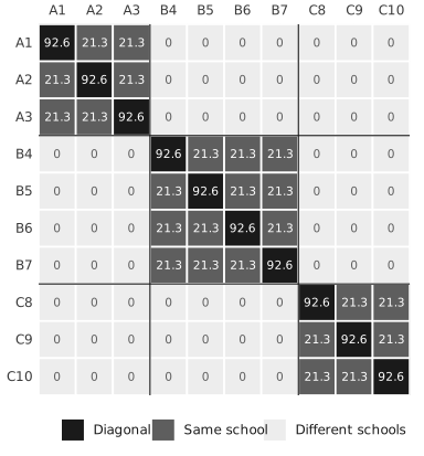
Note. Rows and columns: students of the excerpt, labeled by school (A, B, C) and position. Cell values: model-implied variances (diagonal) and covariances under the random-intercept model with the variance components estimated from all 23 schools, rounded to one decimal. Black: variances; dark gray: covariances within a school; light gray: zero covariances between schools. Black lines separate the school blocks.

Inverses of patterned matrices. Two identities give closed-form inverses and determinants of such matrices. The Woodbury identity states that, for conformable matrices with $\mathbf{A}$ and $\mathbf{C}$ invertible,

and the matrix determinant lemma states that $|\mathbf{A}+\mathbf{U}\mathbf{C}\mathbf{W}|=|{\mathbf{C}}^{-1}+\mathbf{W}{\mathbf{A}}^{-1}\mathbf{U}||\mathbf{C}||\mathbf{A}|$. With $\mathbf{A}={\sigma }^2\mathbf{I}$, $\mathbf{U}={\mathbf{Z}}_j$, $\mathbf{C}=\mathbf{T}$, and $\mathbf{W}={\mathbf{Z}}_j^{\prime }$, the identity gives ${\mathbf{V}}_j^{-1}={\sigma }^{-2}\{\mathbf{I}-{\mathbf{Z}}_j({\sigma }^2{\mathbf{T}}^{-1}+{\mathbf{Z}}_j^{\prime }{\mathbf{Z}}_j{)}^{-1}{\mathbf{Z}}_j^{\prime }\}$, which requires only the inversion of a $q\times q$ matrix. When $\hat{\mathbf{T}}$ is singular, the equivalent form ${\mathbf{V}}_j^{-1}={\sigma }^{-2}\{\mathbf{I}-{\mathbf{Z}}_j\mathbf{T}({\sigma }^2{\mathbf{I}}_q+{\mathbf{Z}}_j^{\prime }{\mathbf{Z}}_j\mathbf{T}{)}^{-1}{\mathbf{Z}}_j^{\prime }\}$ avoids ${\mathbf{T}}^{-1}$. For the random intercept,

For school A with $n_A=3$, the diagonal elements of ${\mathbf{V}}_A^{-1}$ are 0.0118, the off-diagonal elements are $-$0.0022, and $|{\mathbf{V}}_A|=687,552$, the product of the three eigenvalues; direct numerical inversion agrees with Equation (A.5) to within $10^{-14}$ in every element, and the determinant computed by software agrees to within a relative difference of $10^{-14}$. The factor ${\sigma }^2+n_j{\tau }_0^2$ is $n_j$ times the variance of the cluster mean ${\bar{y}}_j$ (Section A.7), and it reappears in the shrinkage factor of Section A.8.

A.6Kronecker Products and Balanced Designs#

The Kronecker product of an $m\times n$ matrix $\mathbf{A}$ and a matrix $\mathbf{B}$ is the block matrix $\mathbf{A}\otimes \mathbf{B}$ whose $(i,k)$ block is $a_{ik}\mathbf{B}$. Its rules are $(\mathbf{A}\otimes \mathbf{B})(\mathbf{C}\otimes \mathbf{D})=\mathbf{A}\mathbf{C}\otimes \mathbf{B}\mathbf{D}$ when the products $\mathbf{A}\mathbf{C}$ and $\mathbf{B}\mathbf{D}$ exist, $(\mathbf{A}\otimes \mathbf{B}{)}^{\prime }={\mathbf{A}}^{\prime }\otimes {\mathbf{B}}^{\prime }$, $(\mathbf{A}\otimes \mathbf{B}{)}^{-1}={\mathbf{A}}^{-1}\otimes {\mathbf{B}}^{-1}$ for invertible $\mathbf{A}$ and $\mathbf{B}$, and, for square $\mathbf{A}$ ($r\times r$) and $\mathbf{B}$ ($s\times s$), $|\mathbf{A}\otimes \mathbf{B}|=|\mathbf{A}{|}^s|\mathbf{B}{|}^r$. In a balanced design with $J$ clusters of $n$ units, the covariance matrix of the random-intercept model is

which shows at once that the clusters are independent and identically structured, and that $|\mathbf{V}|=|{\tau }_0^2{\mathbf{J}}_n+{\sigma }^2{\mathbf{I}}_n{|}^J$. The vec operator, which stacks the columns of a matrix, is linked to the Kronecker product by $\mathrm{vec}(\mathbf{A}\mathbf{B}\mathbf{C})=({\mathbf{C}}^{\prime }\otimes \mathbf{A})\mathrm{vec}(\mathbf{B})$. Kronecker products also describe separable covariance structures, for example for repeated measures of several outcomes, and they also express the covariance matrix ${\mathbf{J}}_{n_j}\otimes \mathbf{T}+{\mathbf{I}}_{n_j}\otimes \mathbf{\Sigma }$ of a cluster in the multivariate multilevel model of Chapter 27 (outcomes stacked within units, complete data); the balanced-design results of Chapters 3 and 16, such as expected mean squares and design effects, can be derived with them.

A.7Expectations and Covariances of Linear Forms#

If $\mathbf{y}$ has mean $\mathbf{\mu }$ and covariance matrix $\mathbf{\Sigma }$, and $\mathbf{A}$, $\mathbf{B}$, and $\mathbf{b}$ are constant, then

For a quadratic form, $E({\mathbf{y}}^{\prime }\mathbf{A}\mathbf{y})=\mathrm{tr}(\mathbf{A}\mathbf{\Sigma })+{\mathbf{\mu }}^{\prime }\mathbf{A}\mathbf{\mu }$; this result underlies the bias of the maximum likelihood variance estimator and its correction by REML (Chapter 9). Applied to the random-intercept model, Equation (A.7) gives the variance of a cluster mean, $\mathrm{Var}({\bar{y}}_j)=1^{\prime }{\mathbf{V}}_{j}1/n_j^2={\tau }_0^2+{\sigma }^2/n_j$, and, divided by $({\tau }_0^2+{\sigma }^2)/n_j$, the design effect $1+(n_j-1)\rho$ of Chapter 16, where $\rho ={\tau }_0^2/({\tau }_0^2+{\sigma }^2)$.

The generalized least squares (GLS) estimator of the fixed effects, for known ${\mathbf{V}}_j$, is a linear form in $\mathbf{y}$:

With the stacked $\mathbf{X}$ and $\mathbf{V}$ of Section A.5, ${\sum }_j{\mathbf{X}}_j^{\prime }{\mathbf{V}}_j^{-1}{\mathbf{X}}_j={\mathbf{X}}^{\prime }{\mathbf{V}}^{-1}\mathbf{X}$ and $\hat{\mathbf{\gamma }}=\mathbf{A}\mathbf{y}$ with $\mathbf{A}=({\mathbf{X}}^{\prime }{\mathbf{V}}^{-1}\mathbf{X}{)}^{-1}{\mathbf{X}}^{\prime }{\mathbf{V}}^{-1}$; the covariance matrix follows from Equation (A.7), because $\mathbf{A}\mathbf{V}{\mathbf{A}}^{\prime }=({\mathbf{X}}^{\prime }{\mathbf{V}}^{-1}\mathbf{X}{)}^{-1}$. In practice the estimated ${\hat{\mathbf{V}}}_j$ replaces ${\mathbf{V}}_j$, and the standard errors ignore the uncertainty of the variance components, which is why the small-sample corrections of Chapter 10 (Satterthwaite or Kenward–Roger degrees of freedom and Kenward–Roger standard errors) are needed with few clusters. For the ten students of the excerpt, Equation (A.8) with the variance components of the full data gives an intercept of 49.35 (SE 4.67) and a homework slope of 4.69 (SE 2.70), against 49.78 and 4.42 from ordinary least squares, which weights all students equally. Because the REML estimate of $\mathbf{\gamma }$ is the GLS estimate evaluated at ${\hat{\mathbf{V}}}_j$, Equation (A.8) applied to all 519 students reproduces the lme4 estimates and standard errors to within $10^{-12}$.

Projection matrices. In ordinary regression, the hat matrix $\mathbf{H}=\mathbf{X}({\mathbf{X}}^{\prime }\mathbf{X}{)}^{-1}{\mathbf{X}}^{\prime }$ projects $\mathbf{y}$ onto the fitted values; it is symmetric and idempotent, and $\mathbf{I}-\mathbf{H}$ produces the residuals. In GLS, the fitted values are ${\mathbf{H}}_V\mathbf{y}$ with ${\mathbf{H}}_V=\mathbf{X}({\mathbf{X}}^{\prime }{\mathbf{V}}^{-1}\mathbf{X}{)}^{-1}{\mathbf{X}}^{\prime }{\mathbf{V}}^{-1}$, which is idempotent but not symmetric, and the residuals are weighted by ${\mathbf{V}}^{-1}$ in the matrix $\mathbf{P}={\mathbf{V}}^{-1}(\mathbf{I}-{\mathbf{H}}_V)$, that is,

which satisfies $\mathbf{P}\mathbf{X}=0$ and $\mathbf{P}\mathbf{y}={\mathbf{V}}^{-1}(\mathbf{y}-\mathbf{X}\hat{\mathbf{\gamma }})$. The REML log-likelihood depends on $\mathbf{y}$ only through ${\mathbf{y}}^{\prime }\mathbf{P}\mathbf{y}=(\mathbf{y}-\mathbf{X}\hat{\mathbf{\gamma }}{)}^{\prime }{\mathbf{V}}^{-1}(\mathbf{y}-\mathbf{X}\hat{\mathbf{\gamma }})$, which does not involve $\mathbf{\gamma }$: up to a constant, ${\ell }_R=-\frac{1}{2}\{\log |\mathbf{V}|+\log |{\mathbf{X}}^{\prime }{\mathbf{V}}^{-1}\mathbf{X}|+{\mathbf{y}}^{\prime }\mathbf{P}\mathbf{y}\}$ (Chapter 9). The CR2 adjustment of cluster-robust standard errors (Chapters 10 and 32) uses the diagonal blocks ${\mathbf{H}}_{jj}$ of the hat matrix, $\mathbf{H}$ for OLS and ${\mathbf{H}}_V$ for GLS.

A.8The Multivariate Normal Distribution#

An $n\times 1$ vector $\mathbf{y}$ with mean $\mathbf{\mu }$ and positive definite covariance matrix $\mathbf{\Sigma }$ is multivariate normal, $\mathbf{y}\sim \mathcal{N}(\mathbf{\mu },\mathbf{\Sigma })$, if its density is

The ML log-likelihood of the multilevel model is the sum over clusters of the logarithm of Equation (A.10) with $\mathbf{\mu }={\mathbf{X}}_j\mathbf{\gamma }$ and $\mathbf{\Sigma }={\mathbf{V}}_j$, which is where the determinants and inverses of Section A.5 enter; the REML log-likelihood of Section A.7 evaluates it at the GLS estimate and adds $-\frac{1}{2}\log |{\mathbf{X}}^{\prime }{\mathbf{V}}^{-1}\mathbf{X}|$, up to a constant (Chapter 9). Three properties are used repeatedly. First, a linear function $\mathbf{A}\mathbf{y}+\mathbf{b}$ of a multivariate normal vector $\mathbf{y}$ is multivariate normal, with the mean and covariance of Equation (A.7); the marginal model follows from Equation (A.1) in this way, because ${\mathbf{u}}_j$ and ${\mathbf{e}}_j$ are independent and therefore jointly normal. Second, uncorrelated elements or subvectors of a multivariate normal vector are independent; for variables that are each normal but not jointly normal, zero correlation does not imply independence. Third, if $\mathbf{y}$ is partitioned into ${\mathbf{y}}_1$ and ${\mathbf{y}}_2$ with mean and covariance

then the conditional distribution of ${\mathbf{y}}_1$ given ${\mathbf{y}}_2$ is normal with

The conditional mean is a linear regression of ${\mathbf{y}}_1$ on ${\mathbf{y}}_2$, and the conditional variance does not depend on the observed ${\mathbf{y}}_2$. The matrix ${\mathbf{\Sigma }}_{11}-{\mathbf{\Sigma }}_{12}{\mathbf{\Sigma }}_{22}^{-1}{\mathbf{\Sigma }}_{21}$ is the Schur complement of ${\mathbf{\Sigma }}_{22}$, which also appears in the inverse of a partitioned matrix; Chapter 12 uses this inverse of the coefficient matrix of Henderson’s mixed-model equations to obtain the prediction-error variances of the random effects, and Appendix B also uses it to obtain the covariance matrix of $\hat{\mathbf{\gamma }}$.

Empirical Bayes predictions as conditional means. The random effects ${\mathbf{u}}_j$ and the outcomes ${\mathbf{y}}_j$ are jointly normal, with $\mathrm{Cov}({\mathbf{u}}_j,{\mathbf{y}}_j)=\mathbf{T}{\mathbf{Z}}_j^{\prime }$. Applying Equation (A.12) with ${\mathbf{y}}_1={\mathbf{u}}_j$ and ${\mathbf{y}}_2={\mathbf{y}}_j$ (so that ${\mathbf{\mu }}_1=0$, ${\mathbf{\mu }}_2={\mathbf{X}}_j\mathbf{\gamma }$, ${\mathbf{\Sigma }}_{11}=\mathbf{T}$, ${\mathbf{\Sigma }}_{12}=\mathbf{T}{\mathbf{Z}}_j^{\prime }$, and ${\mathbf{\Sigma }}_{22}={\mathbf{V}}_j$) gives the conditional mean and variance

With estimates in place of $\mathbf{\gamma }$, $\mathbf{T}$, and ${\sigma }^2$, the conditional mean is the empirical Bayes prediction, and the conditional variance is the posterior variance that lme4 reports, which ignores the uncertainty of $\hat{\mathbf{\gamma }}$ (Chapter 12). For the random intercept, Equation (A.5) reduces these expressions to ${\lambda }_j({\bar{y}}_j-{\bar{\mathbf{x}}}_j^{\prime }\mathbf{\gamma })$ and ${\tau }_0^2{\sigma }^2/({\sigma }^2+n_j{\tau }_0^2)=(1-{\lambda }_j){\tau }_0^2$, where ${\bar{\mathbf{x}}}_j={\mathbf{X}}_j^{\prime }1/n_j$ and ${\lambda }_j=n_j{\tau }_0^2/({\sigma }^2+n_j{\tau }_0^2)$ is the reliability of the cluster mean (Chapter 5, Equation (5.3)) and the shrinkage factor. In the excerpt, school A has ${\lambda }_A=.473$ and a mean residual of $-$2.07 from the GLS fit to the ten students, so its predicted effect is $-$0.98 with a posterior standard deviation of 3.35; school B, with four students, has ${\lambda }_B=.545$, a mean residual of 2.88, and a predicted effect of 1.57. Computed in this way for all 23 schools, the predictions agree with those of lme4.

A.9Derivatives, Information, and the Delta Method#

Newton-type algorithms for maximizing a likelihood, and the standard errors that follow from it, use derivatives with respect to the parameters, and two matrix rules do most of the work. For a covariance matrix $\mathbf{V}(\theta )$ that depends on a parameter $\theta$,

for the random intercept, $\partial {\mathbf{V}}_j/\partial {\tau }_0^2={\mathbf{J}}_{n_j}$ and $\partial {\mathbf{V}}_j/\partial {\sigma }^2={\mathbf{I}}_{n_j}$. The vector of first derivatives of the log-likelihood is the score, and the negative expected matrix of second derivatives is the Fisher information $\mathcal{I}(\mathbf{\psi })$, where $\mathbf{\psi }=({\mathbf{\gamma }}^{\prime },{\mathbf{\theta }}^{\prime }{)}^{\prime }$ collects the fixed effects and the covariance parameters $\mathbf{\theta }$ of Chapter 9. With many clusters, and when the true values lie in the interior of the parameter space (Section A.12), the ML estimator $\hat{\mathbf{\psi }}$ is approximately normal with covariance matrix $\mathcal{I}(\mathbf{\psi }{)}^{-1}$; this is the source of the standard errors of fixed effects and variance components, and Fisher scoring and Newton–Raphson use the same derivatives to find the maximum (Chapter 9).

The delta method gives approximate standard errors for functions of estimates. If $\hat{\mathbf{\theta }}$ is approximately $\mathcal{N}(\mathbf{\theta },{\mathbf{\Sigma }}_{\theta })$ and $g$ is a smooth function with gradient $\nabla g$, then $\mathrm{Var}\{g(\hat{\mathbf{\theta }})\}\approx \nabla g(\mathbf{\theta }{)}^{\prime }{\mathbf{\Sigma }}_{\theta }\nabla g(\mathbf{\theta })$. Two applications are common in multilevel reports: the standard error of a standard deviation from that of a variance, $\mathrm{SE}({\hat{\tau }}_0)\approx \mathrm{SE}({\hat{\tau }}_0^2)/(2{\hat{\tau }}_0)$, and the standard error of the intraclass correlation $\hat{\rho }={\hat{\tau }}_0^2/({\hat{\tau }}_0^2+{\hat{\sigma }}^2)$, whose gradient with respect to $({\tau }_0^2,{\sigma }^2)$ is $({\sigma }^2,-{\tau }_0^2)/({\tau }_0^2+{\sigma }^2{)}^2$. Because the sampling distributions of variance estimates are skewed when the clusters are few, intervals from profile likelihood or the bootstrap are preferable to delta-method intervals for variance components (profile and bootstrap intervals: Chapter 10; the failure of Wald inference for variances: Chapter 11).

A.10The Chi-Square, t, and F Distributions#

If $z_1,\dots ,z_k$ are independent standard normal variables, ${\sum }_i{z}_i^2$ has a chi-square distribution with $k$ degrees of freedom, ${\chi }_k^2$, with mean $k$ and variance $2k$. More generally, if $\mathbf{y}\sim \mathcal{N}(\mathbf{\mu },\mathbf{\Sigma })$ with $n$ elements, the quadratic form $(\mathbf{y}-\mathbf{\mu }{)}^{\prime }{\mathbf{\Sigma }}^{-1}(\mathbf{y}-\mathbf{\mu })$ is ${\chi }_n^2$. This is the basis of the Wald test of $c$ linear hypotheses $\mathbf{L}\mathbf{\gamma }=0$, with $\mathbf{L}$ a $c\times p$ contrast matrix of rank $c$, whose statistic $(\mathbf{L}\hat{\mathbf{\gamma }}{)}^{\prime }\{\mathbf{L}\widehat{\mathrm{Var}}(\hat{\mathbf{\gamma }}){\mathbf{L}}^{\prime }{\}}^{-1}\mathbf{L}\hat{\mathbf{\gamma }}$ is approximately ${\chi }_c^2$ when the clusters are many. The likelihood-ratio statistic $-2({\ell }_0-{\ell }_1)$ of nested models that differ by $c$ parameters has the same approximate distribution when the null values of these parameters lie in the interior of the parameter space; models that differ in their fixed effects must be compared with ML, not REML, log-likelihoods, whereas models with the same fixed part may be compared with either (Chapters 10 and 11).

If $z$ is standard normal and independent of $w\sim {\chi }_k^2$, then $z/\sqrt{w/k}$ has a $t$ distribution with $k$ degrees of freedom; and if $w_1\sim {\chi }_{k_1}^2$ and $w_2\sim {\chi }_{k_2}^2$ are independent, $(w_1/k_1)/(w_2/k_2)$ has an $F$ distribution with $k_1$ and $k_2$ degrees of freedom. In multilevel models, the $t$ and $F$ reference distributions are approximations whose degrees of freedom must be estimated, for example by the Satterthwaite or Kenward–Roger methods of Chapter 10, because the squared standard errors are not exactly scaled chi-square variables independent of the estimates.

A.11Distributions for Discrete Outcomes#

The generalized linear mixed models of Chapters 23 and 24, and the discrete-time hazard models of Chapter 25, replace the normal distribution of the outcome, given the random effects, by distributions for discrete data. A binary outcome is Bernoulli with success probability ${\pi }_{ij}$, mean ${\pi }_{ij}$, and variance ${\pi }_{ij}(1-{\pi }_{ij})$; the number of successes in $m$ independent trials with a common probability ${\pi }_{ij}$ is binomial, with mean $m{\pi }_{ij}$ and variance $m{\pi }_{ij}(1-{\pi }_{ij})$. A count is often modeled as Poisson, with variance equal to its mean $\mu$; a variance larger than the mean is overdispersion, which the negative binomial distribution or an observation-level random effect absorbs (Chapter 24). The Bernoulli, binomial, and Poisson variances are functions of the mean, so that, unlike in the normal model, the level-1 variance is not a separate parameter. The logistic model for a binary outcome can be written as a threshold model for a continuous latent response whose residual has the standard logistic distribution, with mean 0 and variance ${\pi }^2/3\approx 3.29$, where $\pi \approx 3.14159$ is the mathematical constant; this constant replaces ${\sigma }^2$ in the latent-scale intraclass correlation ${\tau }_0^2/({\tau }_0^2+{\pi }^2/3)$ of Chapter 23.

A.12Mixture Distributions for Tests on the Boundary#

The chi-square reference distribution of the likelihood-ratio test requires that the null value of the tested parameters lie in the interior of the parameter space. A variance is bounded below by zero, so the null hypothesis ${\tau }_0^2=0$ places the parameter on the boundary. Under this null hypothesis, and with many clusters, the estimate is zero in about half of the samples (somewhat more often with few clusters, especially under ML; Chapter 11), and the likelihood-ratio statistic is then zero; in the other half it behaves like ${\chi }_1^2$. Its large-sample distribution is therefore the 50:50 mixture of a point mass at zero (${\chi }_0^2$) and ${\chi }_1^2$ (Self & Liang, 1987; Stram & Lee, 1994). When a random slope is added to a model with a random intercept, one variance and one covariance are added, and the reference distribution becomes the 50:50 mixture of ${\chi }_1^2$ and ${\chi }_2^2$. More generally, adding one random effect to a model with $k$ correlated random effects adds one variance and $k$ covariances, the reference distribution is the 50:50 mixture of ${\chi }_k^2$ and ${\chi }_{k+1}^2$, and the $p$ value of an observed statistic $c>0$ is

with $P({\chi }_0^2>c)=0$. Table A.2 gives critical values, and Figure A.2 compares the tail probabilities with those of the naive chi-square distribution. For one variance, the mixture critical value at $\alpha =.05$ is 2.71, which is the 10% critical value of ${\chi }_1^2$: a statistic of 2.71 has $p=.100$ under ${\chi }_1^2$ but $p=.050$ under the mixture, and the usual critical value 3.84 corresponds to $p=.025$. The naive test is thus conservative, and its $p$ values can be halved in this case. When several variances are tested together, the mixture has more components with weights that depend on the information matrix, and simulation or a parametric bootstrap is the practical route (Chapter 11).

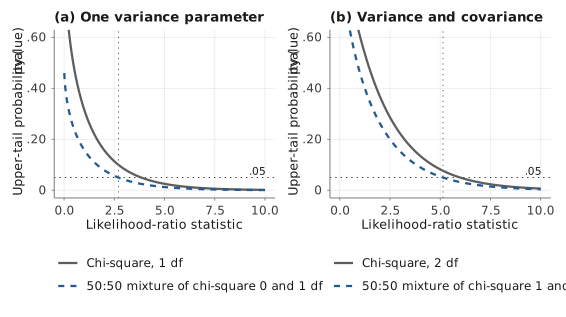
Note. Solid lines: naive chi-square distributions with 1 (panel a) and 2 (panel b) degrees of freedom; dashed lines: 50:50 mixtures of chi-square distributions with 0 and 1 (panel a) and 1 and 2 (panel b) degrees of freedom. Horizontal dotted line, labeled .05: upper-tail probability .05; vertical dotted line: the corresponding critical value of the mixture.

Further Reading#

Searle et al. (1992)

Matrix results and the distribution theory of variance components models.

Pinheiro & Bates (2000)

The matrix formulation of linear mixed models and its computation.

Self & Liang (1987); Stram & Lee (1994)

Likelihood-ratio tests when parameters lie on the boundary.