From ANOVA and Regression to Multilevel Models
In this chapterfixed-effects and random-effects analysis of variance; regression that ignores clusters; within, between, and total regressions; the two-stage approach and its problems; the multilevel model as the repair; fixed-effects regression and cluster-robust standard errors as alternatives.
Readers of this book already know two tools that are routinely applied to grouped data. Analysis of variance (ANOVA) compares group means, and regression relates an outcome to predictors. This chapter applies both tools, one after another, to the same small data set: mathematics scores and homework time of 260 pupils in ten NELS:88 schools. Each analysis answers one question well and fails at another. The failures are instructive, because each one points to a feature of the multilevel model, and by the end of the chapter the multilevel model appears not as a new technique but as the natural repair of the familiar ones. The sequence follows the lecture on “Models for clustered data” that has opened the course for many years (see also Snijders & Bosker, 2012, Ch. 3).
3.1Ten Schools#
The data come from ten of the 23 NELS:88 schools introduced in Chapter 1: 260 pupils in nine public schools and one private school (Table 3.1). School sizes range from 20 to 67 pupils, and mean mathematics scores range from 42.1 to 62.8. The last two columns of the table anticipate Section 3.6: they give the intercept and slope of an ordinary least-squares (OLS) regression of mathematics on homework within each school, with their standard errors.
| Mathematics | Stage-one OLS | ||||||
|---|---|---|---|---|---|---|---|
| School | Sector | Mean | SD | Mean SES | (SE) | (SE) | |
| 7472 | Public | 23 | 45.7 | 7.5 | 0.48 | 50.7 (2.2) | 3.55 (1.25) |
| 7829 | Public | 20 | 42.1 | 8.3 | 0.85 | 49.0 (3.6) | 2.92 (1.33) |
| 7930 | Public | 24 | 53.2 | 11.5 | 0.15 | 38.8 (2.9) | 7.91 (1.37) |
| 24725 | Public | 22 | 43.5 | 10.0 | 0.70 | 34.4 (1.8) | 5.59 (0.82) |
| 25456 | Public | 22 | 49.9 | 8.4 | 0.20 | 53.9 (2.5) | 4.72 (2.20) |
| 25642 | Public | 20 | 46.4 | 4.3 | 1.07 | 49.3 (1.5) | 2.49 (1.11) |
| 62821 | Private | 67 | 62.8 | 5.7 | 1.04 | 59.2 (1.4) | 1.09 (0.39) |
| 68448 | Public | 21 | 49.7 | 10.3 | 0.17 | 36.1 (3.5) | 6.50 (1.46) |
| 68493 | Public | 21 | 46.3 | 9.6 | 0.46 | 38.5 (3.2) | 5.86 (1.99) |
| 72292 | Public | 20 | 47.9 | 11.3 | 0.50 | 37.7 (2.4) | 6.34 (1.12) |
Note. = number of pupils; SES = socioeconomic status (standardized in the full NELS:88 sample); and = intercept and slope of the within-school OLS regression of mathematics on the homework category, with standard errors in parentheses.
Figure 3.1 shows the two extremes of the analyses to come. Panel (a) shows one regression line fitted to all 260 pupils, as if schools did not exist. Panel (b) shows a separate line for each school. The single line rises by about 3.6 points per homework category. The school lines tell a more complicated story: in five schools the line rises steeply, in four it falls, and in the private school (the long line at the top) it rises only slightly.
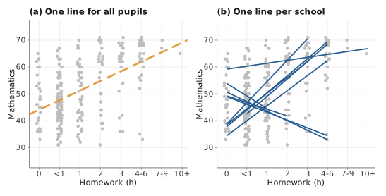
Note. Gray points are pupils, jittered horizontally. Panel (a): the dashed line is the OLS line for all 260 pupils. Panel (b): each solid line is the OLS line of one school, drawn over the range of homework observed in that school.
3.2Analysis of Variance With Schools as Fixed#
Ignore homework for a moment and ask whether mean mathematics differs between the ten schools. The one-way ANOVA model is
where is an overall mean, is the effect of school (with a constraint such as ), and is the deviation of pupil from the mean of school . The school means are estimated by the observed means , and by the within-school mean square. Written as a regression, Equation (3.1) has one dummy variable for each school and no intercept (or an intercept and dummies), and the school effects are ordinary regression coefficients.
Part (a) of Table 3.2 gives the ANOVA table. The ten school means differ far more than the variation among pupils within schools would lead one to expect, , , and the within-school variance is estimated as .
| (a) Analysis of variance | |||||
|---|---|---|---|---|---|
| Source | df | SS | MS | F | p |
| Between schools | 9 | 14,031 | 1,558.9 | 21.55 | |
| Within schools | 250 | 18,086 | 72.3 | ||
| (b) Random-effects estimates | |||||
| Estimator | ICC | ||||
| ANOVA (moments) | 59.00 | 72.34 | .45 | ||
| REML | 34.01 | 72.26 | .32 | ||
Note. df = degrees of freedom; SS = sum of squares; MS = mean square. = estimated between-school variance; = estimated within-school variance; ICC = intraclass correlation. The ANOVA (method-of-moments) estimator is with ; REML = restricted maximum likelihood.
This analysis treats the schools as fixed: the ten schools are the whole population of interest, and the conclusions concern these ten schools and no others. That is appropriate if a school district wants to compare its ten schools. It is not appropriate if the ten schools are a sample and the questions concern schools in general: how much schools differ in the population, or how a school characteristic relates to achievement. The fixed-effects ANOVA has no parameter for “how much schools differ in general,” and because each school has its own parameter, it cannot include a school-level predictor such as sector or mean SES: every school-level variable is perfectly collinear with the school dummies.
3.3Analysis of Variance With Schools as Random#
When the schools are regarded as a random sample from a population of schools, the school effects become random variables. The random-effects ANOVA model is
with and independent. This is the empty multilevel model of Chapters 1 and 2. It has only three parameters, whatever the number of schools: the population mean , the between-school variance , and the within-school variance . As shown in Chapter 2, it implies that every pupil’s score has variance and that every pair of pupils in the same school has covariance (compound symmetry), so the intraclass correlation is the correlation between the scores of two pupils in the same school.
3.3.1Estimating the variance components#
The classical estimators come from the ANOVA table. The expected value of the within-school mean square is , and the expected value of the between-school mean square is , where is a kind of average school size that equals when all schools have pupils (Searle et al., 1992). Equating the mean squares to their expectations gives the method-of-moments (ANOVA) estimators
For the ten schools, and the ICC is .45. Restricted maximum likelihood (REML), the default method in many multilevel programs (Chapter 9), gives and an ICC of .32 (Table 3.2, part b).
Why do the two estimates differ so much? With equal school sizes and a positive ANOVA estimate, the two methods agree. With unequal sizes they weight schools differently. The between-school mean square weights each school’s deviation from the grand mean by its size, so the large private school (67 pupils, with a mean about 15.6 points above the unweighted mean of the other nine schools) dominates it. REML weights each school by the precision with which its mean estimates the population mean, and precision grows much more slowly than school size once is large compared with . The same weighting shows up in the estimate of the overall mean. The mean of all 260 pupils is 51.3, the unweighted mean of the ten school means is 48.8, and the REML estimate () lies between them, much closer to the unweighted mean. With only ten schools every estimate of is imprecise, a point Chapter 16 develops.
3.3.2Complete, no, and partial pooling#
Figure 3.2 places the analyses so far on a single scale. Complete pooling (panel a) ignores schools and estimates one mean for all pupils. No pooling (panel b) estimates a separate, unrelated mean for every school; in the diagram the mean is a diamond inside the school plate, one fixed parameter per school with nothing connecting them. Partial pooling (panel c) treats the school means as draws from a common distribution; the diamond has been promoted to a white circle with a parent and a variance (Chapter 2). The terms are from Gelman & Hill (2007).
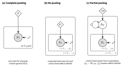
Note. Unified Model Graphs of three models for the mean of . Diamonds are fixed parameters, the white circle is a random school mean with variance loop , shaded circles are observed outcomes, and the short arrows mark the residual variance . In panel (a) a single plate covers all pupils; in panels (b) and (c) the pupil plate is nested in the school plate.
The partially pooled model borrows information across schools. A school’s mean is estimated partly from its own pupils and partly from the other schools, and the fewer pupils a school has, and the larger the within-school variance is relative to the between-school variance, the more its estimate is pulled toward the overall mean. Chapter 12 derives these estimates, known as empirical Bayes or shrinkage estimates. Here it is enough to note that partial pooling is what allows a model to include school-level predictors (the variation of school means is modeled, not absorbed by dummies) and to make statements about the population of schools.
3.4Regression That Ignores Schools#
Now bring homework back. An OLS regression of mathematics on homework for all 260 pupils (Figure 3.1a) gives a slope of 3.57 with a standard error of 0.39. Two things are wrong with this result. The first is the standard error. OLS assumes that the 260 residuals are independent, but pupils in the same school share whatever makes their school different, so the residuals are correlated within schools. As Chapter 1 showed, the OLS standard error is then typically too small. A cluster-robust (sandwich) standard error, which allows arbitrary correlation among the residuals of the same school (Liang & Zeger, 1986), is 0.77 (with the CR1 small-sample adjustment), twice the OLS value: the data contain about a quarter as much information about this slope as OLS assumes, and with only ten clusters even the cluster-robust value is probably too small (Chapter 10).
The second problem is the meaning of the slope. Even with a correct standard error, the pooled slope describes the total relation between homework and mathematics in the 260 pupils. This relation mixes two different things: how pupils who do more homework than their schoolmates differ from those schoolmates, and how schools whose pupils do more homework differ from other schools. The next section separates the two.
3.5Within, Between, and Total Regressions#
Adding the school dummy variables of Equation (3.1) to the regression gives the analysis of covariance (ANCOVA) model
in which each school has its own intercept and all schools share the slope . Because the school intercepts absorb every difference between schools, is estimated only from differences among pupils within schools; it is the pooled within-school slope. For the ten schools (). This model is also called the fixed-effects regression, and it is a widely used way of “controlling for” clusters (Section 3.8).
The complementary analysis regresses the ten school means of mathematics on the ten school means of homework. This between-school regression uses only differences between schools, and its slope is 4.98 (, with 8 degrees of freedom). Schools whose pupils do more homework have much higher mean mathematics, but with ten schools this slope is very imprecise, and the association between schools may reflect many other school differences (the school with the most homework is the private school, which also has the highest mean SES).
The total slope, 3.57, lies between the within slope (2.14) and the between slope (4.98). More precisely, the total OLS slope is a weighted average of the within slope and a between slope in which the school means are weighted by school size (here 7.01, much steeper than 4.98, because the largest school has the highest means of both homework and mathematics), with weights given by the shares of the within-school and between-school sums of squares of homework (.706 and .294: ) (Cronbach, 1976; Snijders & Bosker, 2012). Exercise B3, solved in Appendix G, derives the identity. A predictor whose variance lies mostly within schools gives a total slope close to the within slope, and one whose variance lies mostly between schools gives a total slope close to the between slope. Chapter 7 shows how a multilevel model estimates both slopes at once by including the school mean of the predictor, and why the difference between them, the contextual effect, is often of substantive interest.
3.6The Two-Stage Approach#
Before multilevel software was widely available, a common way to study how relations vary across schools was to proceed in two stages (Burstein, 1980). In stage one, a regression is fitted separately in each school. In stage two, the estimated intercepts and slopes are used as outcomes and regressed on school characteristics. This is the “slopes as outcomes” idea of Chapter 2, carried out by hand.
3.6.1Stage one#
The last two columns of Table 3.1 give the stage-one results. The slopes range from to points per homework category, and their standard errors from 0.39 (the private school, with 67 pupils and a wide range of homework) to 2.20 (school 25456, with 22 pupils who report very little homework). Six slopes are clearly positive and four are negative. The unweighted mean of the ten slopes is 1.96, with a standard error of .
3.6.2Stage two#
Figure 3.3 plots the stage-one estimates against school mean SES, a school-level (compositional) variable. Because homework is not centered, the intercepts are predicted mathematics scores at homework category 0. An unweighted OLS regression of the ten intercepts on mean SES gives a coefficient of 5.12 (), and a regression of the ten slopes gives 1.73 (). Neither is significant, and with ten data points neither could be precise.
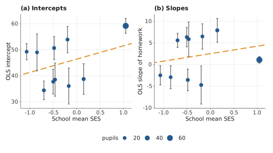
Note. Each point is one school’s stage-one OLS estimate (point area proportional to the number of pupils); vertical bars extend two standard errors on each side. The dashed lines are unweighted OLS regressions of the ten estimates on school mean SES.
3.6.3What is wrong with the two-stage approach#
The figure shows the main problems at a glance. First, the ten estimates are not equally precise: the standard errors of the slopes differ by a factor of more than five, yet the stage-two regression gives each school the same weight. Second, the variation among the estimated slopes has two sources, true differences between school slopes and sampling error in each estimate, and the two-stage approach does not separate them. The standard deviation of the estimated slopes (5.0) therefore overstates how much the true slopes differ. Third, schools with few pupils, or with little variation in the predictor, give unstable estimates, and a school with fewer pupils than regression coefficients cannot be analyzed at all, and one with exactly as many yields no standard errors. Fourth, level-1 variables that happen not to vary in a school (for example, a sex variable in a single-sex school) make the stage-one regression for that school inestimable. Fifth, there is no single model for the whole data set, so there is no likelihood, no overall test, and no way to impose constraints such as a common slope for some variables. Weighting the stage-two regression by the inverse sampling variances fixes the first problem only partly, because the correct weights depend on the unknown variance of the true slopes as well (Raudenbush & Bryk, 2002).
Two-stage regressions remain valuable as exploratory tools. They are the natural way to look at data before fitting a multilevel model (Chapters 4 and 14), and Table 3.1 and Figure 3.3 are exactly the kind of display that should precede any multilevel analysis. As inferential tools they are replaced by the multilevel model.
3.7The Repair: One Model for Both Stages#
The multilevel model estimates both stages at once. For the random intercept and slope model of Chapter 2,
stage one corresponds to the level-1 equation and stage two to the level-2 equations. The difference is that the multilevel model treats the school coefficients as unobserved random quantities with variances and and covariance , estimates those variances separately from the sampling error, and weights each school accordingly.
For the ten schools the random intercept and slope model estimates the average slope as 2.04 (). The large standard error is honest: the slopes differ greatly between schools, and there are only ten schools from which to estimate their average. Table 3.3 and Figure 3.4 collect the seven estimates of “the effect of homework” obtained in this chapter.
| Method | What the estimate describes | Estimate | SE |
|---|---|---|---|
| Pooled OLS | Total relation | 3.57 | 0.39 |
| Pooled OLS, cluster-robust SE | Total relation | 3.57 | 0.77 |
| Between schools (school means) | Between-school relation | 4.98 | 2.42 |
| Fixed effects (school dummies) | Pooled within-school relation | 2.14 | 0.38 |
| Two-stage (mean of school slopes) | Average school slope | 1.96 | 1.57 |
| Random intercept model | Weighted mix of within and between | 2.21 | 0.38 |
| Random intercept and slope model | Average school slope | 2.04 | 1.55 |
Note. Estimates are mathematics points per homework category. SE = standard error: model-based for OLS and fixed effects; cluster-robust (CR1) for the second row; OLS standard error of the regression of the ten school means (8 df) for the between-school row; for the two-stage mean; REML model-based for the two multilevel models.
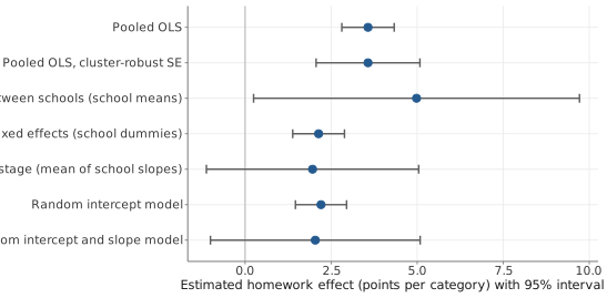
Note. Points are the estimates of Table 3.3; horizontal bars extend 1.96 standard errors on each side ( intervals for the between-school and two-stage rows, with 8 and 9 df, would be 15% to 18% wider). The vertical line marks zero.
The seven rows differ for two reasons, and it is important to keep them apart. Some differ because they estimate different quantities: the total relation (3.57), the between-school relation (4.98), the pooled within-school relation (2.14), and the average of the school-specific slopes (1.96 and 2.04). The random intercept model (2.21) estimates a precision-weighted mix of the within and between relations, which here is close to the within slope because most of the information about homework lies within schools; Chapter 7 shows how to separate the two in a multilevel model. Their standard errors also differ because the methods make different assumptions about the errors: the pooled OLS standard error (0.39) assumes independence and is too small; the cluster-robust standard error (0.77) allows dependence; and the random intercept model’s standard error (0.38) is correct only if the homework slope is the same in every school, which Figure 3.1(b) makes implausible. Among the model-based standard errors, only that of the random slope model allows for the variation of the slopes, and it is four times as large as that of the random intercept model. Chapter 6 returns to this result, which is one of the most important in applied multilevel modeling: omitting a random slope that exists makes the standard error of the corresponding fixed effect too small.
3.7.1How much does the repair gain? A simulation#
With equal cluster sizes and similar spread of the predictor within clusters, the two-stage mean and the multilevel estimate are nearly the same. With unequal sizes they are not. A small simulation shows the difference (Figure 3.5, Table 3.4). Twenty clusters were generated with a standard normal level-1 predictor, a true average slope of 0.30, a random intercept with variance 0.25, and a level-1 variance of 1. The clusters had either balanced sizes (22 or 23) or unbalanced sizes (ten clusters of 5 and ten of 40), with the same total of 450 units, and the slope variance was either 0 or 0.05. Each condition was replicated 1,000 times, and three estimators of the average slope were compared: the two-stage mean, pooled OLS, and the random intercept and slope model.
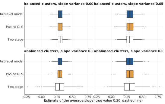
Note. Box plots of 1,000 estimates per estimator and condition; boxes show the quartiles, whiskers extend at most 1.5 interquartile ranges beyond the box, and points mark estimates beyond them. The dashed vertical line marks the true value 0.30. Twenty clusters and 450 units in every condition.
| Cluster sizes | Estimator | Bias | Empirical SD | Mean SE | Coverage | |
|---|---|---|---|---|---|---|
| 0.00 | balanced | Two-stage | 0.002 | 0.050 | 0.050 | .948 |
| 0.00 | balanced | Pooled OLS | 0.002 | 0.052 | 0.052 | .952 |
| 0.00 | balanced | Multilevel model | 0.002 | 0.048 | 0.052 | .959 |
| 0.00 | unbalanced | Two-stage | 0.004 | 0.112 | 0.108 | .965 |
| 0.00 | unbalanced | Pooled OLS | 0.001 | 0.053 | 0.052 | .949 |
| 0.00 | unbalanced | Multilevel model | 0.001 | 0.049 | 0.052 | .957 |
| 0.05 | balanced | Two-stage | 0.000 | 0.073 | 0.070 | .949 |
| 0.05 | balanced | Pooled OLS | 0.001 | 0.078 | 0.054 | .836 |
| 0.05 | balanced | Multilevel model | 0.001 | 0.074 | 0.069 | .926 |
| 0.05 | unbalanced | Two-stage | 0.004 | 0.127 | 0.120 | .941 |
| 0.05 | unbalanced | Pooled OLS | 0.002 | 0.085 | 0.053 | .788 |
| 0.05 | unbalanced | Multilevel model | 0.003 | 0.081 | 0.075 | .912 |
Note. = true slope variance. Bias = mean estimate minus 0.30; Empirical SD = standard deviation of the 1,000 estimates; Mean SE = average estimated standard error; Coverage = proportion of nominal 95% intervals that contain 0.30 ( intervals with 19 df for the two-stage mean, OLS intervals for pooled OLS, Wald intervals for the multilevel model).
All three estimators are essentially unbiased. They differ in precision and in the honesty of their standard errors. With balanced clusters the two-stage mean and the multilevel estimate are equally precise. With unbalanced clusters the two-stage mean is much less precise: its empirical standard deviation is more than twice that of the multilevel estimate when the slopes do not vary (0.112 versus 0.049) and about 1.6 times as large when they do (0.127 versus 0.081), because it gives a cluster of five units the same weight as a cluster of forty. Pooled OLS is about as precise as the multilevel estimate, but when the slopes vary its standard error is far too small, and its 95% intervals contain the true value in only 79% to 84% of the samples. The multilevel model is both efficient and nearly honest; its Wald intervals cover the true value in 91% to 96% of the samples. The slight undercoverage with 20 clusters and a varying slope is a small-sample problem that the corrections of Chapter 10 address.
3.8Two Other Repairs#
The multilevel model is not the only way to handle clustered data, and two alternatives deserve a first look here; Chapters 7 and 32 compare them in detail (Huang, 2016; McNeish et al., 2017).
Fixed-effects regression (Equation (3.4)) includes a dummy variable for every cluster. It removes all between-cluster differences, so its level-1 slopes are pure within-cluster effects and are protected against any confounding by cluster characteristics, observed or not. The price is that no cluster-level variable can be studied (it is absorbed by the dummies), no statement is made about clusters outside the sample, and, unless interactions with every cluster are added, level-1 slopes are assumed to be the same in all clusters. When they are not, the pooled within slope is a weighted average of the cluster slopes, and its standard error, like that of the random intercept model in Table 3.3, describes only the clusters in the sample and understates the uncertainty about the average slope in a population of clusters.
Cluster-robust standard errors keep an ordinary regression (or any other single-level model) but compute standard errors that allow the residuals of the same cluster to be correlated in any way. They repair the standard errors without modeling the dependence. They leave the OLS estimate, and thus the total relation, unchanged; they need a reasonable number of clusters to work well (with few clusters they are themselves too small; Chapter 10), and they give no information about variation between clusters.
The multilevel model represents the dependence explicitly. Its fixed effects can be within, between, or total effects, depending on how the predictors are specified (Chapter 7); it estimates how much clusters differ and how relations vary across clusters; and it supports inference to the population of clusters. The price is that it makes assumptions about the distribution of the random effects and about their independence from the predictors; these assumptions must be checked (Chapters 7 and 15).
Key Terms#
- analysis of covariance (ANCOVA)
- between-cluster regression
- cluster-robust standard error
- complete, no, and partial pooling
- fixed versus random clusters
- fixed-effects regression
- method-of-moments (ANOVA) estimator
- pooled within-cluster slope
- random-effects ANOVA
- stage-one and stage-two regressions
- total regression
- two-stage approach
Exercises#
A. Concept checks#
A clinic network compares patient satisfaction across its eight clinics and wants to know which clinics need attention. Another researcher uses the same data to ask how much clinics differ in general and whether clinic size explains the differences. Which should treat clinics as fixed and which as random? Why?
Explain in your own words why the fixed-effects ANOVA cannot estimate the effect of a school-level variable such as sector.
Using Table 3.3, explain to a colleague why “the effect of homework” has seven different estimates, and which one answers the question “Do pupils who do more homework than their schoolmates score higher?”
Name two situations in which a two-stage analysis cannot be carried out for some clusters.
B. Analytical exercises#
Show that for the random-effects ANOVA, and, for equal cluster sizes , . Derive the moment estimator Equation (3.3). Solution →
Show that the OLS slope in a regression of on with one dummy variable per cluster equals , the pooled within-cluster slope. Solution →
Show that the total OLS slope can be written as , where is the proportion of the sum of squares of that lies between clusters and is the slope of the between-cluster regression weighted by cluster size. Solution →
Using the weights in the Technical Detail box, show that the multilevel estimator of reduces to the unweighted two-stage mean when all are equal, and to the precision-weighted mean when . Solution →
C. Computational exercises#
Reproduce Table 3.2. Then repeat the random-effects analysis for the full 23-school data and compare the ANOVA and REML estimates of .
Reproduce Table 3.3. Add an eighth row: the mean of the stage-one slopes weighted by . Where does it fall, and why? Solution →
Verify numerically the decomposition in exercise B3 for the ten schools.
Carry out the two-stage analysis with sector (public or private) instead of mean SES at stage two. What can and cannot be concluded with one private school?
D. Simulation exercise#
Modify
sim_ch03_twostage_V01.R(save it as_V02) so that the number of clusters is 10 instead of 20, and add the weighted two-stage estimator of exercise C2. How do the precision and coverage of the four estimators change? Relate the result to the ten-school example.
E. Applied mini-project#
Find a published study that used either aggregated data (cluster means) or an individual-level regression that ignored clustering. Rewrite its main analysis as a multilevel model in the three views of Chapter 2. State which of the quantities in Table 3.3 the original analysis estimated and whether its standard errors are likely to be too small.
Lab#
Further Reading#
- Snijders & Bosker (2012, Ch. 3)
-
Fixed and random effects, aggregation, and the within and between regressions.
- Raudenbush & Bryk (2002, Ch. 2–3)
-
The two-stage logic and why the hierarchical linear model improves on it.
- Gelman & Hill (2007, Ch. 12)
-
Complete, no, and partial pooling explained with many graphs.
- Burstein (1980)
-
A classic review of the analysis of multilevel data before multilevel software, including slopes as outcomes.
- Searle et al. (1992)
-
The theory of variance-component estimation, including ANOVA and likelihood estimators in unbalanced data.
- Huang (2016); McNeish et al. (2017)
-
Arguments for cluster-robust and fixed-effects alternatives, and when they are sufficient.