UMG Notation Reference and Figure Style Guide
In this appendixthe lexicon of the Unified Model Graph with its TikZ styles; the drawing rules of the book; parameter promotion across the chapters; the data displays a diagram implies; the style of data figures and of TikZ figures; captions, notes, and numbering; a catalog of the book's diagrams; the source code of the style file and of one diagram.
Every model in this book is drawn as a Unified Model Graph (UMG), the graphical grammar introduced in Chapter 2 (Yu, 2026a), and every data figure follows one visual style. This appendix collects the conventions in one place. It is written for two kinds of readers: those who want to read a diagram or a figure in the book precisely, and those who want to draw their own diagrams and figures in the same way, for a thesis, an article, or a course. The diagrams of the book were drawn in TikZ with a small style file, Style/umg-style.tex, that implements the UMG lexicon; the R package umg (Yu, 2026b) builds, checks, and renders the same diagrams from R.
D.1The Lexicon#
A UMG answers three questions about every quantity in a model, and each answer has its own visual channel (Chapter 2). Fill shows whether a quantity is observed (shaded) or latent (white); shape shows whether it is continuous (circle) or categorical (square); and the border shows its role: a single border for a random variable, a double border for a quantity computed from others, a diamond for a fixed unknown parameter, and a triangle for a known constant. Because the channels are independent, a reader who knows the three questions can read almost any vertex without a legend; the exception is that deterministic vertices are always white, even when they are computed from observed data. Table D.1 lists every element, and Figure D.1 draws each one with the name of its TikZ style.
| Element | Drawn as | Meaning and typical use | Style |
|---|---|---|---|
| Latent continuous variable | White circle | Random effect, latent factor, latent cluster mean | vCL
|
| Observed continuous variable | Shaded circle | Outcome or predictor measured on a continuous scale | vCO
|
| Latent categorical variable | White square | Latent class in a mixture model | vDL
|
| Observed categorical variable | Shaded square | Binary, ordinal, or nominal response or predictor | vDO
|
| Fixed unknown parameter | Diamond | Fixed effect or other fixed parameter, such as a class proportion or a coefficient of a log variance; variances and covariances are written as labels | vP
|
| Deterministic quantity | Double border (circle or square), white | Quantity computed from others, such as an observed cluster mean or a weighted sum | vDetC, vDetD
|
| Known constant | Triangle | Constant 1 of a mean structure, known prior constants, known sampling variances, indicator codes | vK
|
| Explicit residual | Small white circle | Residual that has structure of its own, such as autocorrelation | vEps
|
| Dependence | Single-headed arrow | The head depends on the tail (regression, loading) | eReg
|
| Covariance | Curved double-headed arrow | Symmetric association without direction | eCov
|
| Deterministic assignment | Dashed arrow | The head is computed from the tail | eDet
|
| Mixing | Arrow with an open head | A latent class selects among parameter sets | eMix
|
| Variance loop | Double-headed loop on a vertex | Variance of a random effect | eVar
|
| Residual stub | Short arrow into a vertex | Residual variance of an outcome | \umgstub
|
| Plate | Rounded rectangle | Replication over the units named by its index | plate
|
| Causal badge | Boxed label with a light gray fill | Assumption under which an edge is causal | causalbadge
|
Note. Style: name of the TikZ style (or macro) in Style/umg-style.tex; edge and plate labels use elab, elabplain, and platelab. The triangle for a constant is borrowed from the path diagrams of structural equation modeling, and the plate from graphical models for learning (Buntine, 1994).
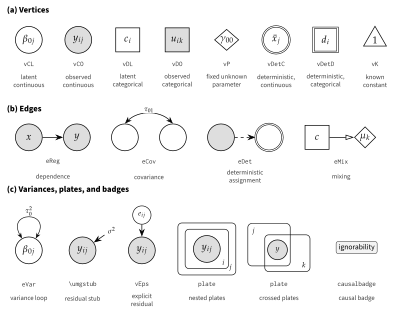
Note. Each element is drawn once; the typewriter label below it is the name of its style in Style/umg-style.tex, and the line below that describes it. Panel (a): vertices. Panel (b): edges. Panel (c): variance marks, the explicit residual, plates, and the causal badge; the right-hand pair of plates overlaps to show crossed classifications.
D.2Drawing Rules#
The lexicon says what each mark means; the drawing rules say where the marks go. Figure D.2 shows a random intercept and slope model with a school predictor, a contextual effect of the observed school mean, and a cross-level interaction, with numbered markers that refer to the rules in Table D.2. The rules make a diagram unambiguous: a reader who follows them can write down the model’s structure from the picture, and a diagram drawn by them corresponds to one model. They describe the usual practice of the book; the two paragraphs after the table give the checks that a diagram must pass and the variants that some chapters need.
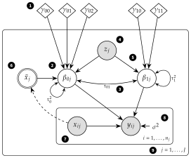
Note. Random intercept and slope model with a school predictor , the observed school mean of the pupil predictor, and a cross-level interaction. Black numbered markers refer to the rules in Table D.2. The coefficient of is , and that of is .
| Rule | Content | First shown |
|---|---|---|
| 1 | A fixed unknown parameter that is the same for every unit is a diamond outside all plates; a fixed slope may instead be written as the label of the edge it multiplies. Fixed parameters that differ across the units of a plate, such as fixed school effects or class-specific parameters, are diamonds inside that plate. Variance and covariance parameters label loops, curved arrows, and stubs. | Figure 2.4 |
| 2 | A coefficient that varies across clusters is a white circle inside the plate of the clusters across which it varies, with a variance loop; the diamonds pointing into it are its mean. | Figures 2.4 and 2.5 |
| 3 | Random coefficients of the same clusters are joined by a curved double-headed arrow, labeled with their covariance. | Figure 2.4 |
| 4 | An observed cluster-level predictor is a shaded vertex inside the cluster plate and outside the unit plate; its effect on the cluster’s mean outcome is an arrow into the random intercept, not into the unit-level outcome. | Figure 2.4 |
| 5 | A cross-level interaction is an ordinary arrow from the cluster-level predictor into the random slope; no arrow points at another arrow. | Figures 1.7 (proposition) and 6.6 (model) |
| 6 | A quantity computed from the data, such as an observed cluster mean, has a double border and is fed by dashed arrows; a latent cluster mean is a white circle instead. | Figure 5.6 |
| 7 | Observed unit-level variables are shaded vertices inside the innermost plate. | Figure 1.2 |
| 8 | The residual variance of an outcome is a short stub labeled with the variance; a residual with structure of its own is drawn as an explicit vertex. | Figures 2.4 and 20.5 |
| 9 | A plate is labeled with its index and, where useful, its range, normally at its lower right; where plates overlap or share a corner, or another element occupies it, the label moves to a free corner. Nested plates express hierarchy. | Figure 1.2 |
A well-formed diagram also defines a probability model. Every random vertex has a distribution given the vertices that point to it, and the joint distribution of the random quantities, given the parameters and the observed predictors, is the product of these conditional distributions, replicated as the plates indicate (Chapter 2). This reading gives three checks for any diagram: every random vertex must have a stated distribution given its parents; no chain of single-headed arrows may lead from a vertex back to itself; and every quantity in the model’s equations must appear as a vertex or as a label.
Several chapters extend the rules for their models. In the cross-classified and multiple-membership models of Chapter 26 and in several later chapters, the diagrams use a mixed form: additive random effects of each classification and the cluster predictors point into the outcome, directly (Figure 26.2) or through weighted sums (Figure 26.5), and fixed slopes are written as edge labels; Figure 1.7 draws substantive propositions rather than models and uses the same short form. Occasions nested in persons form a plate like any other level (Figure 19.3), but when successive residuals depend on each other the occasion plate is unrolled, because a plate cannot show dependence between its replicates (Figure 20.5). Crossed classifications are drawn as overlapping plates, with the units that belong to both classifications in a dotted plate at the intersection (Figure 26.2). Multiple membership joins separate unit and cluster plates through dashed edges labeled with the membership weights into double-bordered weighted sums (Figure 26.5). In a Bayesian model every parameter becomes a random vertex whose parents are triangles of known prior constants (Figure 13.1), and in a mixture model a latent class selects among class-specific parameters through mixing edges (Figure 22.4). The within-between decomposition is drawn with dashed arrows from the observed predictor into a double-bordered cluster mean (Figures 5.6b, 7.3a, and 21.2a) and, where the predictor is centered, a double-bordered deviation (Figures 5.6b and 21.2a); with latent centering, the observed predictor instead receives arrows from a latent cluster mean and a latent deviation (Figures 7.3b and 21.2b). Growth models can also be drawn in a flattened form, with the occasion plate unrolled into one indicator per occasion (Figure 22.1b), and two-level factor models as two single-level diagrams, one for the within and one for the between covariance matrix, instead of in nested plates (Figure 29.1b). Edges into categorical outcomes may carry a link or threshold label, and factor loadings are written on their edges. Labels of loops and stubs are omitted where the variances are not the point of the figure. Some diagrams draw a binary predictor as a circle, such as the school sector in Figures 5.6 and 6.6 and the treatment in Figure 31.3; Figure 18.1 draws the sector as a square, as the lexicon prescribes. Causal badges attach the identifying assumption to the coefficient whose causal reading depends on it (Figure 31.3). Finally, diagrams that report a fitted model print the estimates next to the parameters, edges, and loops, and their source files state where the numbers come from (Figures 18.1 and 19.3).
D.3Parameter Promotion Across the Book#
Parameter promotion is the idea that fixed and random effects are two positions of one parameter (Chapter 2). The same coefficient appears as a diamond outside the plates when it is fixed, as a white circle inside a plate when it varies across the units of that plate, as a random vertex with a prior when it is estimated by Bayesian methods, and as one of several class-specific diamonds in a mixture. Table D.3 follows the move through the book; each row is one position, and the figures show the position in a particular model.
| Position | Diagram | Figures |
|---|---|---|
| Fixed effect | Diamond outside all plates | 2.5(a), 5.2(b) |
| Fixed cluster effect | One diamond per cluster inside the cluster plate | 3.2(b), 5.2(a) |
| Random coefficient | White circle in the cluster plate with a variance loop; the diamond becomes its mean | 2.4, 2.5(b) |
| Predicted random coefficient | Cluster-level vertices point into the random coefficient (level-2 effects and cross-level interactions) | 5.6, 6.6 |
| Coefficient with a prior | Random vertex whose parents are triangles of known prior constants | 2.5(c), 13.1 |
| Class-specific coefficient | A latent class selects among class-specific diamonds through mixing edges | 2.5(d), 22.4 |
| Random coefficient of a variance | A random effect points into the log of the residual variance | 28.2 |
| Random coefficient as a latent variable | Cluster-level random intercepts of several outcomes are latent variables that serve as indicators of a between-level factor | 29.1, 30.1 |
| Random coefficient of a crossed classification | Random effects of items or of a second classification in their own plate | 26.2, 30.3 |
| Random treatment effect | The treatment coefficient varies across sites | 16.4(b), 31.6 |
Note. Figures: figure numbers in the chapters of the book; letters refer to panels.
D.4The Data Displays a Diagram Implies#
Read backward, a diagram is a checklist of data displays: each element implies a display that shows whether the element is needed and whether its assumptions are plausible (Chapters 2 and 4). Table D.4 pairs the elements with their displays and points to examples in the book. The displays are most useful before a model is fitted, to decide which elements it needs, and after it is fitted, to check the elements it has.
| Element | Display | Examples |
|---|---|---|
| Plate | Small multiples: one panel per cluster | 2.6(a), 4.3 |
| Random intercept | Cluster means or intercepts, sorted, with intervals (caterpillar display) | 4.5, 5.1, 12.6 |
| Random slope | Cluster regression lines on common axes (spaghetti display) | 2.6(b), 4.6, 6.1 |
| Random slope (variance) | Variance of the outcome against the predictor with the random slope (variance function) | 2.2, 4.7, 6.2 |
| Covariance of random coefficients | Cluster intercepts against cluster slopes | 2.6(c) |
| Cluster-level predictor | Cluster means against the predictor, or by group | 4.4(c), 5.1, 5.4 |
| Cross-level interaction | Cluster slopes or predicted lines by the cluster-level predictor | 4.4(c), 6.7 |
| Residual stub | Level-1 residuals against fitted values and predictors | 15.1, 15.4 |
| Unrolled occasions | Residual correlations by lag and the variogram | 4.8, 20.3 |
| Deterministic cluster mean | Within-cluster and between-cluster regressions | 5.4 |
Note. Examples: figure numbers in the chapters of the book; letters refer to panels.
D.5The Style of Data Figures#
The data figures of the book are drawn with ggplot2 (Wickham, 2016) and share one theme, one palette, and one export function, defined in Style/mlmbook_figtheme_V01.R; every figure script sources this file first. The theme is a minimal one in Source Sans Pro, with recessive grid lines, thin axis lines, and the legend at the bottom unless direct labels or a free corner of the panel serve better. Its default base size is 10 points; most figures use 8.5 or 9 points, which keeps the tick labels and legend text at about 7 points at print size, also in figures that are exported wider than the text block and scaled down. The purpose of the theme is that the data, not the frame, carry the ink.
The palette (Table D.5) is chosen so that every figure reads correctly in grayscale print as well as on screen. The two series colors differ strongly in lightness: in CIE , which approximates the gray level that a color takes in grayscale print, the blue has 37 and the orange 70. Identity is never carried by color alone. A figure with two series uses the blue and the orange together with different point shapes (filled circle, filled triangle, filled square, open circle, in that order) or line types (solid, dashed, long dashed, dotted), and labels the series directly or in a legend. A single series is drawn in blue or gray; many background series, such as the regression lines of 160 schools, are drawn in thin, partly transparent gray (for example, Figures 4.6 and 6.1) or in light gray (Figure 5.4); and bands and fills are drawn in pale gray. The orange has too little contrast against white to be used for text, so it is used only for marks.
| Name | Hex | Swatch | Use | |
|---|---|---|---|---|
blue
| #245A8F
|
| 37 | First series or a single series; dark in grayscale |
orange
| #E39B3F
|
| 70 | Second series; light in grayscale, always with a second encoding |
grey
| #5E5E5E
|
| 40 | Single series, many-group lines, reference lines |
ink
| #1A1A1A
|
| 9 | Text and axes |
light
| #BDBDBD
|
| 77 | Background data, many-group spaghetti |
pale
| #E6E6E6
|
| 91 | Fills and bands |
Note. Name: name in mlm_col. : CIE lightness (D65 white point) computed from the hexadecimal value, from 0 (black) to 100 (white); as a working rule, colors that differ by more than about 20 units remain distinguishable in grayscale print.
Every data figure is exported three times by save_mlm_fig(): as PDF (vector, for the book and for print), as PNG at 300 dpi (for slides and the web), and as SVG (for the planned web book). The default width is 5.7 inches, the width of the text block, and the height is set for each figure; half of the data figures are exported wider, up to 6.3 inches, and are scaled down when they are included. A few practical rules keep the figures consistent. Axis limits are best set with coord_cartesian() rather than with scale limits, because scale limits remove data outside them and change smoothers and summaries computed from the data; scale limits, which many of the book’s figure scripts still use, are safe only when no data fall outside them. Mathematical labels use plotmath expressions, such as expression(tau[0]^2), which set subscripts and superscripts in the same way on every graphics device; Unicode subscript and superscript characters depend on the font, and the default pdf() device of R replaces most of them, such as the subscript digits, with dots. Scripts are written in ASCII, with Unicode escapes where a Greek letter or a minus sign is needed, and are run in a UTF-8 locale. Two aesthetics, such as color and line type, share one legend only when their titles, breaks, and labels agree, and a layer whose key glyph differs, such as error bars, is drawn with show.legend = FALSE so that it does not alter the legend keys.
D.6The Style of TikZ Figures#
Diagrams, flowcharts, annotated output, and other figures that are not plots of data are drawn in TikZ. Of the 203 figures in Chapters 1 to 32 and Appendices A to C, 71 are TikZ figures and 132 are drawn in R; 48 of the TikZ figures, in 27 chapters, are Unified Model Graphs. Each TikZ figure is a standalone document in Scripts/ChNN/ that loads Source Sans Pro for labels and, except in five figures without model notation (the flowcharts of Figures 9.6, 14.1, 16.2, and 17.5 and the folder tree of Figure 18.4), New PX for text and mathematics; all Unified Model Graphs and four other diagrams also input the style file umg-style.tex. Each is compiled by Scripts/Shared/build_tikz_figure.sh into the same three formats as the data figures:
bash Scripts/Shared/build_tikz_figure.sh \
     Scripts/Ch06/fig06_06_crosslevel_umg_V01.tex Figures/Ch06/fig06_06_crosslevel_umg
The drawing of a diagram is kept in black and gray, so that it needs no color at all; observed vertices are filled with 13% black. Four TikZ figures that report results (Figures 11.3, 13.3, 30.4, and 32.4) are written by the R script that computes them, so that their numbers cannot drift from the results; the two diagrams that print estimates (Figures 18.1 and 19.3) state in their header which results file the numbers come from. Section D.9 reproduces the style file and the source of Figure D.2.
D.7Captions, Notes, and Numbering#
Figures and tables follow the style of the APA Publication Manual (American Psychological Association, 2020). The number (for example, Figure 6.6) is set in bold above the figure or table, and the title on the next line in italic title case; the figure or table follows, and a note, introduced by Note., is set below it and aligned left. In LaTeX, the caption and the label come before the image, and the note is placed outside the centered block, as in this schematic example:
\begin{figure}[tbp]
\caption{Unified Model Graph of the Cross-Classified Random-Effects Model}
\label{fig:ch26-crossed}
{\centering\includegraphics[width=\linewidth]{fig26_02_crossed_umg.pdf}\par}
\fignote{Overlapping plates: ... (mechanics only)}
\end{figure}
A figure note describes the mechanics of the figure: what the axes, symbols, line types, shading, and abbreviations mean. It does not report results, which belong in the text. Tables use horizontal rules only (\{}toprule, \{}midrule, \{}bottomrule) and have their notes below; the notes define symbols and abbreviations and do not repeat the text.
Figures and tables are numbered by chapter, normally in the order of their first citation in the text; in Chapters 20 and 23 a later figure, and in Chapters 10, 18, and 32 a later table, is mentioned in passing before an earlier one. The files follow the same numbering: the file fig06_06_crosslevel_umg is Figure 6.6, and its source is Scripts/Ch06/fig06_06_crosslevel_umg_V01.tex; a data figure is written by an R script, either a figure script with the same stem or the analysis or table script that computes the figure’s content. A check of all 203 figures found zero figures whose file number differs from the figure number. When a figure is inserted in a later version, the following files are renumbered together with the figures, so that the file name always tells where a figure appears.
D.8Catalog of the Diagrams#
Table D.6 lists the 48 Unified Model Graphs of the book with their source files. Together they form a visual index of the models: the random intercept, random slope, and three-level models of Part II, the longitudinal and generalized linear mixed models of the later chapters, and the latent variable, measurement, and causal models of Part VII all appear in the same grammar, and the source file of any of them is a starting point for a new diagram.
| Figure | Title | Source file |
|---|---|---|
| 1.2 | Where Variables Live: Three Data Structures Drawn With Plates | fig01_02_plates_preview
|
| 1.7 | Types of Multilevel Propositions Drawn With Plates | fig01_07_propositions_umg
|
| 2.3 | The Lexicon of the Unified Model Graph | fig02_03_umg_lexicon
|
| 2.4 | The Empty, Random Intercept, and Random Intercept and Slope Models as Unified Model Graphs | fig02_04_three_models_umg
|
| 2.5 | Parameter Promotion: One Coefficient in Four Positions | fig02_05_parameter_promotion
|
| 3.2 | Complete Pooling, No Pooling, and Partial Pooling of School Means | fig03_02_pooling_umg
|
| 4.9 | Plates Are Loops: The Random Intercept and Slope Model as a Graph and as a Data-Generating Program | fig04_09_plates_as_loops
|
| 5.2 | Analysis of Covariance With Fixed School Effects and the Random Intercept Model | fig05_02_ancova_vs_ri_umg
|
| 5.6 | Random Intercept Models With School-Level Predictors | fig05_06_level2_umg
|
| 6.6 | Random Intercept and Slope Model With School Predictors of the Intercept and the Slope | fig06_06_crosslevel_umg
|
| 7.3 | Manifest and Latent Cluster Means in a Random Intercept Model | fig07_03_manifest_latent_umg
|
| 8.2 | The Empty Three-Level Model as a Unified Model Graph | fig08_02_empty_threelevel_umg
|
| 8.4 | A Three-Level Model With Predictors at Each Level and a Pupil-Level Slope That Varies Over Classes and Schools | fig08_04_threelevel_slopes_umg
|
| 10.1 | A Joint Hypothesis About Fixed Effects as a Pair of Unified Model Graphs | fig10_01_hypothesis_umg
|
| 12.1 | Predicting a Random Intercept on the Unified Model Graph | fig12_01_posterior_umg
|
| 13.1 | The Random Intercept and Slope Model Estimated by ML or REML and as a Bayesian Hierarchical Model | fig13_01_bayes_umg
|
| 16.4 | Unified Model Graphs of a Cluster-Randomized Trial and a Multisite Trial | fig16_04_trial_umg
|
| 17.2 | An Imputation Model That Omits the Random Slope and a Substantive-Model-Compatible Model | fig17_02_congeniality_umg
|
| 18.1 | The HSB Final Model as a Unified Model Graph With Its Estimates | fig18_01_hsb_final_umg
|
| 19.3 | The Unconditional Linear Growth Model as a Unified Model Graph | fig19_03_growth_umg
|
| 20.5 | A Random Intercept Model With First-Order Autoregressive Residuals as a Unified Model Graph | fig20_05_ri_ar1_umg
|
| 21.2 | Unified Model Graphs of the Within-Between Decomposition of a Time-Varying Predictor | fig21_02_decomposition_umg
|
| 21.4 | Unified Model Graph of the Multilevel AR(1) Model With Random Inertia | fig21_04_ar1_umg
|
| 21.6 | Unified Model Graph of a Two-Level Dynamic Structural Equation Model | fig21_06_dsem_umg
|
| 21.7 | Unified Model Graph of the Random Intercept Cross-Lagged Panel Model | fig21_07_riclpm_umg
|
| 22.1 | Unified Model Graphs of the Linear Growth Model in Plate Form and in Flattened Form | fig22_01_plate_flat_umg
|
| 22.3 | Unified Model Graph of a Second-Order Latent Growth Model | fig22_03_secondorder_umg
|
| 22.4 | Unified Model Graph of a Growth Mixture Model | fig22_04_gmm_umg
|
| 23.1 | Unified Model Graphs of the Two-Level Logistic Random Intercept Model | fig23_01_logistic_umg
|
| 24.2 | Unified Model Graph of the Two-Level Cumulative Logit Model | fig24_02_ordinal_umg
|
| 24.4 | Unified Model Graph of the Two-Level Baseline-Category Logit Model | fig24_04_multinomial_umg
|
| 24.6 | Unified Model Graphs of the Zero-Inflated and Hurdle Count Models | fig24_06_zero_umg
|
| 25.3 | Unified Model Graph of the Multilevel Discrete-Time Hazard Model | fig25_03_hazard_umg
|
| 26.2 | Unified Model Graph of the Cross-Classified Random-Effects Model | fig26_02_crossed_umg
|
| 26.5 | Unified Model Graph of the Multiple-Membership Model | fig26_05_mm_umg
|
| 27.1 | Unified Model Graphs of the Bivariate Two-Level Model | fig27_01_mv_umg
|
| 27.2 | Unified Model Graphs of the Actor-Partner Interdependence Model | fig27_02_apim_umg
|
| 27.3 | Unified Model Graph of the Random-Effects Meta-Regression Model | fig27_03_meta_umg
|
| 28.2 | Unified Model Graph of the Mixed-Effects Location-Scale Model | fig28_02_mels_umg
|
| 29.1 | Unified Model Graphs of a Two-Level Factor Model in Plate Form and in Flattened Form | fig29_01_twolevel_umg
|
| 29.2 | Unified Model Graph of the Doubly Latent Contextual Model | fig29_02_doubly_latent_umg
|
| 29.4 | Unified Model Graph of 1-1-1 Multilevel Mediation With Within and Between Paths | fig29_04_mediation_umg
|
| 30.1 | Unified Model Graph of a Two-Level Factor Model | fig30_01_mcfa_umg
|
| 30.3 | Unified Model Graph of the Rasch Model With Crossed Person and Item Effects | fig30_03_rasch_umg
|
| 30.6 | Unified Model Graph of an Explanatory Item Response Model | fig30_06_explanatory_umg
|
| 30.7 | Unified Model Graph of a Multilevel Rasch Model With DIF Across Schools | fig30_07_mlirt_umg
|
| 31.3 | Unified Model Graph of the Within-Between Model With Causal Badges | fig31_03_wb_causal_umg
|
| 31.6 | Unified Model Graphs of a Cluster-Randomized Trial and a Multisite Cluster-Randomized Trial | fig31_06_trials_umg
|
D.9Source Code#
The style file defines every element of Table D.1. It is input in the preamble of each Unified Model Graph and of four other diagrams; its comments refer to the tables and sections of the UMG manuscript (Yu, 2026a):
% ============================================================
% Title:  UMG TikZ lexicon: visual primitives of the Unified
%         Model Graph (UMG) system
% File:   umg-style.tex
% Author: H.-T. Yu
% Date:   2026-06-12
% ============================================================
% Input this file in the preamble of any document (manuscript or
% standalone figure) that draws UMG diagrams. Requires TikZ.
%
% Channel-to-attribute mapping (see Table 2 of the manuscript):
%   Fill (luminance) -> observability  (shaded = observed; white = latent)
%   Shape            -> support        (circle = continuous; square = categorical)
%   Border           -> role           (single = random variable; double = deterministic)
%   Diamond          -> fixed unknown parameter (frequentist target of estimation)
%   Triangle         -> known constant (e.g., the unit constant for means)
%   Rounded box      -> plate (exchangeable replication; nesting = hierarchy)
% ------------------------------------------------------------
\usetikzlibrary{arrows.meta,positioning,fit,backgrounds,shapes.geometric,calc}

\tikzset{
  % ----- Vertex primitives -----------------------------------------
  % continuous latent random variable: white circle
  vCL/.style={draw, circle, minimum size=9.5mm, inner sep=1pt, line width=0.7pt, fill=white},
  % continuous observed random variable: shaded circle
  vCO/.style={draw, circle, minimum size=9.5mm, inner sep=1pt, line width=0.7pt, fill=black!13},
  % categorical latent random variable (e.g., latent class): white square
  vDL/.style={draw, rectangle, minimum size=8.5mm, inner sep=2pt, line width=0.7pt, fill=white},
  % categorical observed random variable (e.g., item response): shaded square
  vDO/.style={draw, rectangle, minimum size=8.5mm, inner sep=2pt, line width=0.7pt, fill=black!13},
  % fixed unknown parameter: open diamond
  vP/.style={draw, diamond, aspect=1.15, minimum size=7.5mm, inner sep=0.5pt, line width=0.7pt, fill=white},
  % deterministic node: double border (shape follows support)
  vDetC/.style={draw, circle, double, double distance=1.1pt, minimum size=9.5mm, inner sep=1pt, line width=0.5pt, fill=white},
  vDetD/.style={draw, rectangle, double, double distance=1.1pt, minimum size=8.5mm, inner sep=2pt, line width=0.5pt, fill=white},
  % known constant: triangle (RAM heritage); label inside
  vK/.style={draw, isosceles triangle, isosceles triangle apex angle=60,
             shape border rotate=90, minimum size=7mm, inner sep=0.5pt,
             line width=0.7pt, fill=white},
  % small disturbance/residual node (continuous latent, reduced size)
  vEps/.style={draw, circle, minimum size=6.5mm, inner sep=0.5pt, line width=0.6pt, fill=white},
  % ----- Edge primitives -------------------------------------------
  % stochastic/functional dependence (regression, loading)
  eReg/.style={->, >={Stealth[length=2.8mm]}, line width=0.7pt},
  % covariance / unanalyzed association (symmetric)
  eCov/.style={<->, >={Stealth[length=2.5mm]}, line width=0.7pt},
  % deterministic assignment
  eDet/.style={->, >={Stealth[length=2.8mm]}, line width=0.7pt, dashed},
  % mixing edge: latent class -> parameter set (open arrowhead)
  eMix/.style={->, >={Triangle[open, length=3mm]}, line width=0.7pt},
  % variance stub: double-headed self-loop on a node
  eVar/.style={<->, >={Stealth[length=2mm]}, line width=0.6pt, looseness=5},
  % edge parameter label
  elab/.style={font=\small, fill=white, inner sep=1pt, sloped=false},
  elabplain/.style={font=\small, inner sep=1.5pt},
  % ----- Plates ------------------------------------------------------
  plate/.style={draw, rounded corners=4pt, inner sep=9pt, line width=0.6pt},
  platelab/.style={anchor=south east, inner sep=4pt, font=\small\itshape},
  platelabnw/.style={anchor=north west, inner sep=4pt, font=\small\itshape},
  % ----- Auxiliary ---------------------------------------------------
  dist/.style={font=\footnotesize, text=black!70, inner sep=1pt},
  causalbadge/.style={draw, rounded corners=2pt, font=\footnotesize\sffamily,
                      inner sep=2.5pt, fill=black!5},
}

% Residual stub: arrow into #1 from direction #2 (angle), with label #3.
% Compact abbreviation for an explicit disturbance node; see Section 4.5.
\newcommand{\umgstub}[3]{%
  \draw[eReg] ($(#1)+(#2:0.95)$) -- (#1);
  \node[elabplain] at ($(#1)+(#2:1.25)$) {#3};%
}
The source of Figure D.2 shows a complete diagram. Vertices are placed at explicit coordinates, so that the layout does not depend on automatic placement; the plates are fitted around their vertices on the background layer; and the plate labels are placed at the lower-right corners of the plates:
\documentclass[border=3pt]{standalone}
\usepackage[T1]{fontenc}
\usepackage{newpxtext,newpxmath}
\usepackage[scale=0.95]{sourcesanspro}
\usepackage{tikz}
\input{umg-style.tex}
\tikzset{mk/.style={circle, fill=black, text=white, font=\sffamily\bfseries\scriptsize, inner sep=0.6pt, minimum size=3.6mm}}
\begin{document}
\begin{tikzpicture}
% parameters outside all plates
\node[vP] (g00) at (0.0,6.0) {$\gamma_{00}$};
\node[vP] (g01) at (1.1,6.0) {$\gamma_{01}$};
\node[vP] (g02) at (2.2,6.0) {$\gamma_{02}$};
\node[vP] (g10) at (4.6,6.0) {$\gamma_{10}$};
\node[vP] (g11) at (5.7,6.0) {$\gamma_{11}$};
% cluster level
\node[vCL] (b0) at (1.1,2.6) {$\beta_{0j}$};
\node[vCL] (b1) at (5.1,2.6) {$\beta_{1j}$};
\node[vCO] (z)  at (3.1,4.0) {$z_j$};
\node[vDetC] (xb) at (-0.9,2.6) {$\bar x_j$};
% unit level
\node[vCO] (x) at (1.6,0.2) {$x_{ij}$};
\node[vCO] (y) at (4.3,0.2) {$y_{ij}$};
% edges
\draw[eReg] (g00) -- (b0); \draw[eReg] (g01) -- (b0); \draw[eReg] (g02) -- (b0);
\draw[eReg] (g10) -- (b1); \draw[eReg] (g11) -- (b1);
\draw[eReg] (z) -- (b0); \draw[eReg] (z) -- (b1);
\draw[eDet] (x) to[bend left=25] (xb);
\draw[eReg] (xb) -- (b0);
\draw[eReg] (b0) -- (y); \draw[eReg] (b1) -- (y); \draw[eReg] (x) -- (y);
\draw[eCov] (b0) to[bend right=12] node[elab, below]{\scriptsize $\tau_{01}$} (b1);
\draw[eVar] (b0.205) to[out=205, in=255, looseness=6] node[elabplain, below left]{\scriptsize $\tau_0^2$} (b0.255);
\draw[eVar] (b1.30) to[out=30, in=-30, looseness=6] node[elabplain, right]{\scriptsize $\tau_1^2$} (b1.330);
\umgstub{y}{0}{$\sigma^2$}
\begin{scope}[on background layer]
  \coordinate (yr) at ($(y)+(1.55,0)$);
  \node[plate, fit=(x)(y)(yr), inner xsep=16pt, inner ysep=12pt] (pi) {};
  \node[plate, fit=(pi)(b0)(b1)(z)(xb), inner xsep=22pt, inner ysep=16pt] (pj) {};
\end{scope}
\node[platelab, font=\scriptsize\itshape] at (pi.south east) {$i=1,\dots,n_j$};
\node[platelab, font=\scriptsize\itshape] (jlab) at (pj.south east) {$j=1,\dots,J$};
% numbered markers (Table D.2)
\node[mk] at (-0.75,6.25) {1};
\node[mk] at (0.35,3.25) {2};
\node[mk] at (3.75,2.05) {3};
\node[mk] at (3.75,4.55) {4};
\node[mk] at (4.4,3.65) {5};
\node[mk] at (-1.7,3.25) {6};
\node[mk] at (1.0,-0.45) {7};
\node[mk] at (6.0,0.62) {8};
\node[mk, left=2pt of jlab] {9};
\end{tikzpicture}
\end{document}