Three Views of One Model: Notation, Equations, and Graphs
In this chapterthe notation used in the book; the hierarchical, mixed, and marginal ways of writing a multilevel model; the Unified Model Graph; parameter promotion; the data displays a model implies; what software needs to be told.
A student fits the same multilevel model in three programs and receives three outputs that look nothing alike. One program reports “level-1” and “level-2” coefficients, another reports “fixed effects” and “random effects,” and a third reports a covariance matrix called . The student concludes that the programs fit different models. They do not. Each program shows one of three equivalent ways of writing the same model: as a set of equations, one for each level (the hierarchical view); as a single equation with a fixed part and a random part (the mixed view); and as a statement about the mean and covariance of the outcome (the marginal view). This chapter introduces the notation used throughout the book, shows how the three views follow from one another, and adds a fourth, graphical view: the Unified Model Graph. Being able to move among the four views is the most useful skill for reading multilevel models, and every later chapter relies on it.
2.1Notation#
Table 2.1 lists the symbols used in this book. The notation follows Snijders & Bosker (2012) and Raudenbush & Bryk (2002) closely, with one simplification: random variables are written in lower case (, , ) so that the same letters can be used in the equations, in the diagrams, and in the R code. The last column of the table gives the symbols used in other books and in software output, so that readers can move between sources.
| Symbol | Meaning | Other common notation |
|---|---|---|
| Indices and sample sizes | ||
| , | Level-1 unit (pupil, occasion), level-2 unit (school, person) | and reversed in some texts |
| , , | Units in cluster ; number of clusters; | for clusters in S&B |
| Variables | ||
| Outcome of unit in cluster | (S&B, R&B) | |
| , | Level-1 predictor(s), | |
| , | Level-2 predictor(s), | (R&B), |
| Coefficients and random effects | ||
| , | Intercept and slope of cluster (level-1 coefficients) | , |
| Fixed effects: first subscript names the level-1 coefficient, second the level-2 predictor | ||
| , | Level-2 random effects (cluster deviations) | (S&B), (R&B) |
| Level-1 residual | (S&B), (R&B), | |
| Variance components | ||
| , | Variances of and | , (R&B, HLM) |
| Covariance of and | ||
| Variance of | ||
| Intraclass correlation, | ICC, | |
| Matrices for cluster | ||
| , | outcome and residual vectors | |
| , | Design matrices of the fixed and the random part | |
| , | Vector of fixed effects; vector of random effects of cluster | , (statistics) |
| , | Covariance matrix of ; marginal covariance matrix of | , (SAS: , ) |
Two conventions deserve attention from the start. First, the subscript always refers to the level-1 unit and to the level-2 unit, so is the outcome of unit in cluster . In longitudinal data (Part V) the level-1 unit is a measurement occasion and the level-2 unit is a person; the subscripts keep the same meaning. Second, the fixed effects carry two subscripts. The first says which level-1 coefficient is being modeled ( for the intercept, for the first slope, and so on), and the second says which level-2 predictor it multiplies ( for the constant). Thus is the overall intercept, is the average slope of , is the effect of the level-2 predictor on the intercepts, and is the effect of on the slopes (a cross-level interaction).
2.2The Hierarchical View#
The hierarchical view writes one equation for the level-1 units within each cluster and one equation for each cluster-specific coefficient. It is the most natural way to state a multilevel theory, because it places each variable at its own level. For a model with one level-1 predictor and one level-2 predictor , the level-1 model is an ordinary regression within cluster :
Each cluster has its own intercept and its own slope . The residual is the deviation of unit from its cluster’s regression line, and is the within-cluster residual variance, assumed to be the same in every cluster.
The level-2 model treats the cluster-specific coefficients as outcomes and relates them to cluster characteristics:
with
and the random effects independent of the residuals and independent across clusters. In words: a cluster’s intercept is predicted from , and is what is left over; a cluster’s slope is also predicted from , and is what is left over. The variances and describe how much intercepts and slopes vary across clusters after is taken into account, and the covariance describes whether clusters with high intercepts tend to have high or low slopes.
The hierarchical view makes the substantive meaning of each parameter clear. It also shows immediately where a level-2 variable can enter (only in the level-2 equations) and what a cross-level interaction is (a level-2 variable in the equation for a slope). Its weakness is that it hides what the model says about the outcome itself: Equations (2.1) to (2.3) do not show directly how depends on , or how two outcomes in the same cluster are related.
2.3The Mixed View#
Substituting the level-2 equations into the level-1 equation gives a single equation:
This is the linear mixed model. The fixed part contains the regression coefficients , which are the same for all clusters; the random part contains the random effects , , which vary across clusters, and the residual . The mixed view shows three things that the hierarchical view hides. The cross-level interaction appears as an ordinary product term, . The level-2 predictor appears as an ordinary predictor of the outcome, . Finally, the error term is no longer a single residual but a sum, , whose random-effect terms and are shared by all units of cluster . This composite error is the formal source of the dependence discussed in Chapter 1.
The mixed view is also the form in which models are written in most software. In the R package lme4 (Bates et al., 2015), for example, the model of Equation (2.5) is written y ~ x * z + (x | school): the fixed part outside the parentheses and the random part inside them, with the grouping factor after the vertical bar.
2.3.1The mixed model in matrix form#
For computation and for later chapters it helps to stack the equations of cluster in vectors and matrices (Laird & Ware, 1982):
Here is the vector of outcomes, is the design matrix of the fixed part, is the vector of fixed effects, is the design matrix of the random part, is the vector of random effects, and is the vector of level-1 residuals. For a cluster with three units the model of Equation (2.5) reads
The columns of are the variables that have random coefficients (here the constant and ); they are usually a subset of the columns of . In a model with only a random intercept, , a column of ones.
2.4The Marginal View#
The random effects and are not observed. What is observed is the outcome, and the model makes a statement about its distribution once the random effects are integrated out. This is the marginal model. From Equation (2.6), and because and have mean zero and are independent,
and outcomes in different clusters are uncorrelated. The marginal mean is the fixed part of the mixed model; the marginal covariance matrix collects everything the random part implies about variances and covariances. Because clusters are independent, the covariance matrix of all outcomes is block diagonal, with one block for each cluster.
2.4.1Random intercept models: compound symmetry#
With a random intercept only, and , so . Every outcome has the same variance, , and every pair of outcomes in the same cluster has the same covariance, , whatever the values of the predictors. This pattern is called compound symmetry. The correlation between any two units of the same cluster is the intraclass correlation of Chapter 1, now computed after the predictors in the fixed part have been taken into account (a residual or conditional ICC).
2.4.2Random slope models: the variance function#
With a random slope the picture changes. Writing out Equation (2.8) for single elements gives
The variance of the outcome is now a quadratic function of , the variance function, and the covariance between two units of the same cluster depends on their values of . A random slope therefore makes the marginal model heteroscedastic by construction: at values of where the cluster regression lines fan out, the outcome varies more; where they come closest together, it varies less. The minimum of the variance function lies at . Chapter 6 develops these results in detail.
Figure 2.1 makes Equation (2.8) concrete. It shows the model-implied correlation matrix of mathematics scores for nine NELS:88 pupils, three from each of three schools, chosen to have the lowest, median, and highest homework time in their school. The estimates come from the models fitted in Section 2.5. Under the random intercept model (panel a) the matrix has the compound-symmetry pattern: blocks of equal correlations (.23) within schools and zeros between schools. Under the random intercept and slope model (panel b) the within-school correlations depend on homework. Two pupils with similar and fairly high homework in the same school correlate strongly (.59 and .78 in schools 2 and 3), but a pupil who does no homework and one who does much homework are negatively correlated in the same school (, ). The negative values reflect the crossing of school regression lines seen in Figure 1.3 of Chapter 1: in schools where pupils without homework do well, pupils with much homework do relatively poorly, and vice versa.
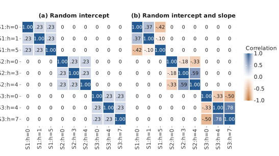
Note. Rows and columns are pupils, labeled by school (S1 = 24725, S2 = 6467, S3 = 62821) and homework category . Cell shading runs from orange (negative) through white (zero) to blue (positive) and each cell prints the correlation. Pairs of pupils in different schools have zero model-implied correlation.
Figure 2.2 shows the corresponding variance functions. Under the random intercept model the variance of mathematics scores is the same (92.6) at every value of homework. Under the random intercept and slope model it is 115.7 for pupils with no homework, falls to a minimum of 72.8 between the categories “less than one hour” and “one hour,” and rises steeply for pupils with much homework. The dotted line marks the within-school part , which is constant; everything above it comes from differences between schools, and under the random slope model the between-school share depends on the value of the predictor.
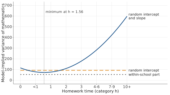
Note. The dashed line shows the variance implied by the random intercept model; the solid curve shows the variance function of the random intercept and slope model, Equation (2.9); the dotted line shows its level-1 variance . The thin vertical line marks the minimum of the variance function. Tick labels give the hours per week represented by each homework category.
2.5Moving Among the Three Views: A Worked Example#
This section fits three models to the NELS:88 data of Chapter 1 (519 pupils in 23 schools) and writes each of them in the three views, using the estimates. The outcome is mathematics achievement, and the level-1 predictor is the homework category (0 = none, 1 = less than one hour, 2 = one hour, and so on up to 7 = ten hours or more per week). The models are the empty model (M0), a random intercept model with homework (M1), and a random intercept and slope model with homework (M2). Table 2.2 shows the estimates, obtained by restricted maximum likelihood (REML; Chapter 9) with lme4.
| Parameter | Symbol | Empty (M0) | Random intercept (M1) | Random intercept and slope (M2) |
|---|---|---|---|---|
| Fixed effects | ||||
| Intercept | 50.76 (1.15) | 46.36 (1.16) | 46.33 (1.76) | |
| Homework | 2.40 (0.28) | 1.98 (0.93) | ||
| Variance components | ||||
| Intercept variance | 26.12 | 21.34 | 62.42 | |
| Slope variance | 17.73 | |||
| Intercept–slope covariance | 27.59 | |||
| Level-1 variance | 81.24 | 71.28 | 53.29 | |
| REML deviance | 3,798.7 | 3,729.3 | 3,635.6 | |
| Parameters | 3 | 4 | 6 | |
Note. Estimates are REML estimates; standard errors in parentheses. = number of estimated parameters (fixed effects and variance components). REML deviances can be compared only between models with the same fixed part (here M1 and M2; see Chapter 11).
library(lme4)
nels <- read.csv("nels88_school23.csv")
M0 <- lmer(math ~ 1 + (1 | school), data = nels)                   # empty model
M1 <- lmer(math ~ homework + (1 | school), data = nels)            # random intercept
M2 <- lmer(math ~ homework + (homework | school), data = nels)     # random intercept and slope
summary(M2)       # fixed effects, variance components, correlation of random effects
VarCorr(M2)$school # the matrix T; sigma(M2)^2 gives sigma^2Each view answers different questions. The hierarchical view says what happens in a typical school and how schools differ. In the average school, the expected mathematics score increases by about 2 points per homework category, but schools differ a great deal: the standard deviation of the slopes is 4.2, so in a school one standard deviation above the average the slope is about , and in a school one standard deviation below it is about . If the slopes are normally distributed, about a third of schools in the population () have a negative slope. The strong negative correlation between intercepts and slopes () says that schools whose pupils do well without homework tend to have flat or negative homework slopes, which matches the pattern of the two schools in Figure 1.3.
The mixed view says what the software estimates as fixed effects (46.33 and 1.98) and which terms are random. Comparing M1 and M2 in Table 2.2 shows something that will recur in Chapter 6: when the slope is allowed to vary, the estimated average slope changes (from 2.40 to 1.98), and its standard error becomes more than three times larger (from 0.28 to 0.93). The random intercept model treats the homework effect as the same in every school and therefore overstates the precision of the average effect.
The marginal view says what the model implies about the observed scores: the population-average regression line and the variances and correlations shown in Figures 2.1 and 2.2. It also shows how the variance components make up the total variance. In the empty model the total variance is , of which 24% lies between schools. Adding homework as a fixed effect (M1) reduces both components ( to 21.3 and to 71.3). Allowing the slope to vary (M2) moves variance out of (to 53.3) and into the school-level part, which now depends on homework. How to summarize such changes as “explained variance” is taken up in Chapter 11.
2.6Drawing the Model: The Unified Model Graph#
Equations are precise but hard to scan; path diagrams are easy to scan but, in their usual form, cannot show which coefficients vary across clusters. This book draws every model as a Unified Model Graph (UMG), a formally specified graphical grammar in which a well-formed diagram corresponds to one statistical model (Yu, 2026a). The R package umg (Yu, 2026b) builds, checks, and renders such diagrams. The grammar answers three questions about every quantity in a model and uses one visual channel for each answer.
2.6.1Three questions about every quantity#
Figure 2.3(a) shows the vertices. Is the quantity observed? Observed variables are shaded; unobserved (latent) quantities, including random effects, are white. Is it continuous or categorical? Continuous quantities are circles; categorical quantities (a binary response, a latent class) are squares. What role does it play? A random variable has a single border; a fixed unknown parameter, the target of frequentist estimation, is a diamond; a known constant is a triangle; and a quantity computed deterministically from others, such as a cluster mean , has a double border.
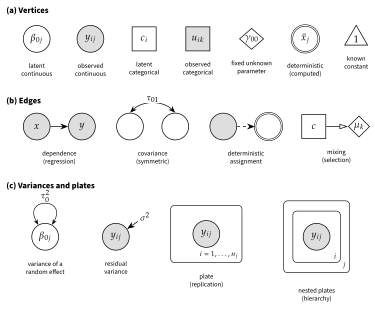
Note. Panel (a): vertex types. Fill encodes observability (shaded = observed, white = latent), shape encodes support (circle = continuous, square = categorical), and border encodes role (diamond = fixed unknown parameter, triangle = known constant, double border = deterministic). Panel (b): edge types. Panel (c): a variance loop on a random effect, a residual stub on an observed outcome, a plate, and nested plates. Adapted from Yu (2026a).
Figure 2.3(b) shows the edges. A single-headed arrow is a dependence: the quantity at the head depends on the quantity at the tail, as in a regression. A curved double-headed arrow is a covariance, a symmetric association with no direction. A dashed arrow into a double-bordered vertex is a deterministic assignment. An arrow with an open head from a latent class to a set of parameters is a mixing edge, used for mixture models (Chapter 22). Figure 2.3(c) shows two shorthand marks, a loop for the variance of a random effect and a short arrow for a residual variance, and the plates introduced in Chapter 1.
2.6.2The core models as UMGs#
Figure 2.4 draws three models: the empty model M0 (panel a), a random intercept model with a pupil predictor and a school predictor (panel b; without and it is M1), and the random intercept and slope model M2 (panel c). In every panel the pupil plate () is nested in the school plate (), observed pupil variables are shaded circles inside the pupil plate, the observed school variable (panel b) is a shaded circle inside the school plate but outside the pupil plate, the random coefficients ( in panels a and b, and in panel c) are white circles in the school plate, and the fixed effects are diamonds outside all plates. In panel (b) the slope is fixed, so its diamond points directly at . Reading panel (c) from top to bottom reproduces the hierarchical view: the population parameters and generate the school coefficients and , which vary across schools with variances and and covariance ; the school coefficients and the pupil’s predictor (homework, written in the worked example) generate the pupil’s score , with residual variance .
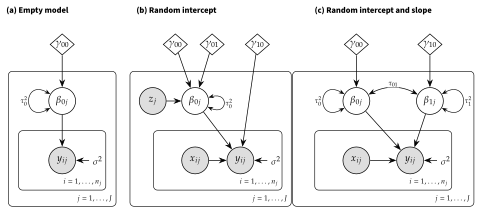
Note. Diamonds are fixed effects, placed outside all plates. White circles in the school plate are school-specific coefficients; loops on them mark their variances and the curved double-headed arrow in panel (c) marks their covariance. Shaded circles in the pupil plate are observed pupil variables; the shaded circle in panel (b) is an observed school variable. The short arrow into marks the level-1 residual variance.
A UMG is not only a picture. Every vertex with incoming arrows has a distribution given the vertices that point to it, and the joint distribution of the random quantities in the diagram, given the parameters and observed predictors, is the product of these conditional distributions, replicated as the plates indicate. For panel (c) this product is
which is exactly the hierarchical model of Equations (2.1) to (2.4) without . Integrating the white (unobserved) random coefficients out of Equation (2.11) gives the marginal model. In this sense the diagram carries all three views: the arrows give the hierarchical equations, the white vertices mark the random part of the mixed model, and removing them by integration gives the marginal model.
2.7Parameter Promotion: Fixed and Random as Two Positions#
The most useful single idea in the UMG grammar is parameter promotion (Yu, 2026a). Figure 2.5 shows one coefficient, the effect of on , in four positions. In panel (a) the coefficient is a diamond outside both plates: one fixed slope for all schools. In panel (b) the diamond has been moved into the school plate and has become a white circle with a distribution across schools, ; the old diamond remains as the mean of that distribution. This single move is the difference between a fixed and a random effect. In panel (c) the coefficient has been given a prior distribution with known constants (the triangle), which is how Bayesian estimation treats every parameter (Chapter 13). In panel (d) a latent class vertex selects one of several class-specific versions of the coefficient through a mixing edge, which is how mixture models work (Chapter 22).
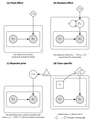
Note. Each panel shows a pupil plate () nested in a school plate (). (a) Fixed effect: a diamond outside the plates. (b) Random effect: a white circle in the school plate with a variance loop, whose mean is the diamond. (c) Bayesian prior: the coefficient is a random vertex whose parent is a triangle of known prior constants. (d) Class-specific: a latent class (white square) selects among class-specific diamonds through an open-headed mixing edge. Adapted from Yu (2026a).
The statistical content of this idea is not new. Random effects are latent variables (Curran, 2003; Mehta & Neale, 2005; Skrondal & Rabe-Hesketh, 2004), a prior turns a parameter into a random variable, and a mixture switches parameters with a latent class. What the diagrams add is that the four cases look different on the page while the move between them is a single relocation. Readers who have understood panel (b) have understood what a random effect is, and they will recognize the same move when it reappears for random intercepts (Chapter 5), random slopes (Chapter 6), Bayesian estimation (Chapter 13), growth mixtures (Chapter 22), and latent variables in multilevel structural equation models (Chapter 29).
2.8The Data Displays a Model Implies#
Every element of a UMG implies a display of the data that would show whether that element is needed (Yu, 2026a). A plate implies small multiples: one panel per cluster, so that the within-cluster relation can be seen in each. A random coefficient implies a display of the cluster-specific estimates of that coefficient: for a random slope, a “spaghetti” plot of cluster regression lines. A covariance edge between two random coefficients implies a scatterplot of one set of cluster-specific estimates against the other. A random slope also implies a variance function, as in Figure 2.2. Read forward, a diagram is a model to be fitted; read backward, it is a checklist of displays to look at before and after fitting.
Figure 2.6 shows the three displays implied by panel (c) of Figure 2.4 for the NELS:88 data. The small multiples (panel a) show that the within-school relation between homework and mathematics is roughly linear but differs clearly from school to school. The school-specific least-squares lines (panel b) show the spread of intercepts and slopes around the pooled line, which motivates the random intercept and the random slope. The scatterplot of school intercepts against school slopes (panel c) shows a strong negative association (the correlation of the 23 pairs of least-squares estimates is ), which is what the covariance edge represents and what the model estimates, net of sampling error, as . Chapter 4 develops these displays systematically, and the function umg_eda_scaffold() in the umg package generates them from a diagram and a data set.
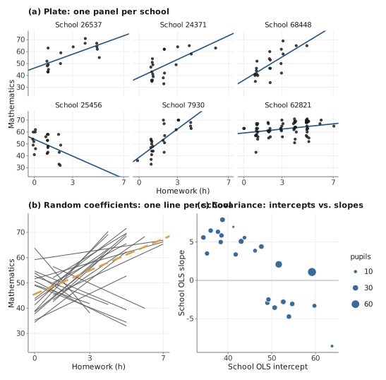
Note. Panel (a): mathematics against homework category for six schools, with each school’s least-squares line; points are jittered horizontally. Panel (b): least-squares lines of all 23 schools, drawn over the observed range of homework in each school; the dashed line is the pooled least-squares line. Panel (c): least-squares intercept against least-squares slope for each school; point area is proportional to the number of pupils.
2.9What Software Needs to Be Told#
Every program for multilevel models asks for the same four pieces of information, although in different ways: (1) the outcome and the fixed part (which predictors, which interactions); (2) the grouping variable that defines the clusters; (3) the random part (which coefficients vary across clusters); and (4) the structure of the covariance matrix of the random effects (whether the random intercept and slope may be correlated). Most programs also allow a covariance structure to be specified for the level-1 residuals, which becomes important for longitudinal data (Chapter 20), and all of them require an estimation method, set explicitly or by default (Chapter 9).
Programs written around the mixed view (R, SAS, SPSS, Stata, JASP) take a single model statement with a fixed part and a random part. Programs written around the hierarchical view (HLM) take a level-1 equation and level-2 equations. Programs written around latent variables (Mplus) take a within-cluster model and a between-cluster model in which the random coefficients appear as latent variables, which is exactly the picture in Figure 2.4(c). The software crosswalk at the end of this section gives the syntax for model M2 in each program, and Table 2.3 shows where each variance component appears in their output.
| Program | , | ||
|---|---|---|---|
R (lme4)
| school (Intercept) and homework under Variance; standard deviations also printed
| printed as a correlation (Corr), not a covariance | Residual
|
SAS (MIXED)
| UN(1,1), UN(2,2) in Covariance Parameter Estimates
| UN(2,1)
| Residual
|
SPSS (MIXED)
| UN (1,1), UN (2,2)
| UN (2,1)
| Residual
|
Stata (mixed)
| var(_cons), var(homework)
| cov(homework,_cons)
| var(Residual)
|
| Mplus | between-level variances of MATH and S
| WITH statement for MATH and S (between level)
| within-level residual variance of MATH
|
| HLM 8 | and in the matrix |
Note. Labels are those printed for the model in the crosswalk box below; they can change with the order of terms in the model statement and between program versions. = intercept variance; = slope variance; = intercept–slope covariance; = level-1 residual variance.
2.10How to Read the Rest of This Book#
From now on every new model is presented in a “three views” box like the one in Section 2.5, drawn as a UMG, and accompanied by the data displays it implies. When a result is easier to see in one view, the text uses that view. Interpretation of coefficients and the theory behind a model are usually clearest in the hierarchical view. Software syntax, interactions, and the effect of centering (Chapter 7) are clearest in the mixed view. Estimation (Chapter 9), tests of variance components (Chapter 11), covariance structures for longitudinal data (Chapter 20), and comparisons with population-average models such as generalized estimating equations (Chapters 23 and 32) are clearest in the marginal view. The UMG is the view to return to when a model becomes complicated, because it shows at a glance which quantities vary at which level.
Key Terms#
- compound symmetry
- covariance matrix of random effects ()
- design matrix (, )
- fixed effect
- fixed part
- hierarchical (level-specific) view
- level-1 model
- level-2 model
- linear mixed model
- marginal covariance matrix ()
- marginal model
- model-implied data display
- parameter promotion
- plate
- random effect
- random part
- slopes as outcomes
- Unified Model Graph (UMG)
- variance function
Exercises#
A. Concept checks#
For each statement, say whether it belongs to the hierarchical, the mixed, or the marginal view: (a) “Each school has its own regression of anxiety on workload.” (b) “The variance of anxiety increases with workload.” (c) “The model contains the product of school climate and workload.” (d) “Two teachers in the same school have correlated anxiety scores, and the correlation is larger when both have a high workload.” (e) “The slope of workload is predicted by school climate.” (f) “The error term is .”
In Figure 2.4(b), explain why is drawn inside the school plate but outside the pupil plate, and why is drawn outside both plates.
A colleague reports the correlation between the random intercept and slope as and concludes that “schools with high achievement benefit less from homework.” What additional information is needed before this interpretation can be judged? (Hint: see the pitfall on where .)
Which of the following change when a level-1 predictor with a random slope is shifted by a constant: , , , , , , the deviance?
B. Analytical exercises#
Consider the hierarchical model , with , , and . (a) Write the mixed model and identify its fixed and random parts. (b) Write , , and for a cluster with three units. (c) Derive for this cluster. Solution →
Show that under a random intercept model has compound symmetry, and find the correlation between any two units of the same cluster. Solution →
For the random slope model, show that the variance function Equation (2.9) has its minimum at , and compute the minimum value. Using the M2 estimates, verify the values 115.7 (at ) and 72.8 (at the minimum) reported in the text. Solution →
Show that if is replaced by , the random slope model with parameters is equivalent to a model with , , and . Solution →
C. Computational exercises#
Fit M0, M1, and M2 to the NELS:88 data in R and reproduce Table 2.2. Then fit M2 in one other program from the crosswalk, once with the default covariance structure and once with an unstructured one, and explain the differences.
Using the M2 estimates, compute the model-implied covariance matrix for a school with four pupils whose homework categories are 0, 1, 3, and 6, and convert it to a correlation matrix. Which pairs of pupils are negatively correlated, and why? Solution →
Center homework at its grand mean and refit M2. Compare , , and the deviance with those in Table 2.2, and check the results against exercise B4.
Draw M2 as a UMG with the
umgpackage, both by hand withumg_model()and withumg_from_lmer(), and runumg_validate()on each. Then produce the displays of Figure 2.6 withumg_eda_scaffold().
D. Simulation exercise#
Write a script (with the book’s header and block structure) that simulates 5,000 schools of four pupils each from M2, with the M2 estimates as true values and homework fixed at 0, 1, 3, and 6 within every school. Compute the empirical covariance matrix of the four scores across schools and compare it with the matrix you derived in exercise C2. How large must the number of simulated schools be for the two to agree to one decimal place? Solution →
E. Applied mini-project#
Choose a published article that reports a two-level model with at least one random slope. (a) Write the model in the three views, using the published estimates where they are reported. (b) Draw it as a UMG. (c) List what the article does not report that you needed for (a), for example the covariance of the random effects or the centering of the predictors. (d) Write a two-sentence comment to the authors about the missing information.
Lab#
Further Reading#
- Snijders & Bosker (2012, Ch. 4–5)
-
The random intercept and random slope models in the notation followed here, with the hierarchical and mixed forms side by side.
- Raudenbush & Bryk (2002, Ch. 2)
-
The level-by-level formulation and the “slopes as outcomes” idea, as implemented in the HLM program.
- Laird & Ware (1982)
-
The paper that established the matrix formulation for longitudinal data.
- Verbeke & Molenberghs (2000, Ch. 3)
-
A careful treatment of the difference between the hierarchical and the marginal model.
- Singer (1998)
-
A classic tutorial that maps the hierarchical view onto SAS
PROC MIXEDsyntax; still the best bridge between the two for SAS users. - Bates et al. (2015)
-
The formula syntax and computational approach of
lme4. - Curran (2003); Mehta & Neale (2005)
-
Why random effects are latent variables, and what this means for connecting multilevel models to structural equation models.
- Yu (2026a)
-
The Unified Model Graph, including parameter promotion and model-implied displays.